Sensorless Real-Time Reduced Order Model Based Adaptive Maximum Power Tracking Pitch Controller for Grid Connected Wind Turbines

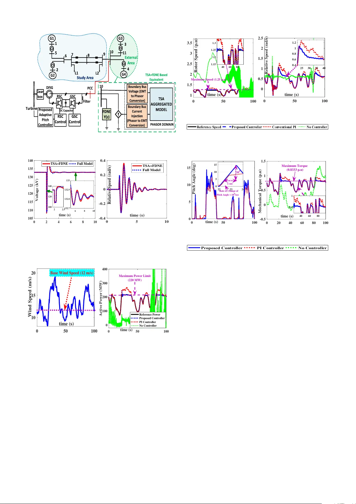
Sensorless Real-Time Reduced Or der Model Based Adaptive Maxim um P o wer T rac king Pitch Contr oller for Grid Connected Wind T urbines Abilash Thakallapelli 1 , Sudipta Ghosh 1 , Sukumar Kamalasadan 1 ∗ 1 Electrical and Computer Engineering, UNC Char lotte, Charlotte, USA * E-mail: skamalas@uncc.edu Abstract: This paper presents a sensor-less maximum pow er trac king (MPT) pitch controller for g rid connected Wind T urbine (WT). The main advantage of the proposed architecture is that the approach ensures smooth operation and thus minimizes the mechanical stress and damage on the WT during high wind speed and grid transient conditions. Simultaneously , it also: a) reduces transients in P oint of Common Coupling (PCC) b us v oltage, b) reduces rotor speed oscillations, and c) controls the output power of the wind turbine without exceeding its thermal limits. The approach can work without wind speed measurements. In order to consider the eff ect of grid variations at the PCC , the affected area in the grid is modeled as a study area (area of interest), and remaining area (external area) is modeled as frequency dependent reduced order model (FDROM). The reduced order model (ROM) is then used to estimate the reference speed. The proposed controller is designed using the error between actual speed of the generator and the reference speed, to ensure smooth oper ation and limit the speed and aerodynamic power at the r ated values . The architecture is ev aluated using wind f ar m integrated Kundur’ s two-area and IEEE-39 bus test systems using real-time digital simulator (R TDS). 1 Introduction In recent years, the mov e towards eliminating fossil fuel depen- dency and embracing sustainable energy based power generation has increased interest in inte grating renew able energy sources (RES) into the power grid. In 2016, WTG provided almost 6% of U.S. electricity generation (about 37% of electricity generation from RES) [1]. How- ev er , WTGs operate under varying wind conditions and depends on time and geographical location, which may be above or below rated values, thus varying their output power . During high wind speed con- ditions, the controller should limit the speed of the generator not crossing the rated value by limiting the rotation rate of the rotor, since pitch system contributes to 21.3% of the overall failure rate of wind turbines [2]. This can be achieved by controlling the blade pitch angle [3]. Howe ver , in practical systems, WTG operations are also influenced by the dynamics of the entire power grid. Thus, the design of WTG controllers should tak e into consideration of grid dynamics. W ind speed conditions are generally measured using anemometers, failure of which can cause deterioration in tracking performance. This should be addressed in the controller design as well [4]. Grid le vel interactions of the wind farms/turbines are gener - ally controlled considering a constant voltage at the PCC even though electro-mechanical dynamics are included in such simula- tions. This ignores response of the wind farms with the electro- magnetic transients in the grid. The effect is on the mechanical fatigue that happens on the wind generators. If one should design a controller considering grid dynamics, detailed Electro-Magnetic T ransient (EMT) based grid models with dynamic models of WTG including DFIG are required. Howe ver , detail modeling of large scale po wer grid is impractical due to computational complexity [5]. In [5, 6], to reduce computational burden sev eral model order reduc- tion techniques based on linearized models have been developed, but these models are effectiv e only during low-frequenc y oscillations. A possible method to reduce computational burden while retaining accuracy is to model part of WTG integrated grid (study area) in detail and the remainder of the network (external area) [7] as an equiv alent. For this, the external area is modeled as a combination of low frequenc y (Transient Stability Assessment -TSA type) and high frequency (FDNE type) equi valents. In TSA type, the network is for- mulated as an admittance matrix at the fundamental frequency , and the generators are aggregated and modeled in detail such that low- frequency electromechanical oscillations are preserved, whereas the high-frequency oscillations are preserv ed by FDNE. In the literature, several WTG pitch control strategies for limit- ing the aerodynamic power and generator speed are proposed. An individual pitch control scheme with a proportional-integral (PI) controller with two resonant compensators is proposed in [8]. How- ev er , the PI controllers are designed based on a specific operating point. A pitch angle controller based on fuzzy logic is proposed in [9], in which generator output power and speed are used as input to the controller . Howe ver , determining exact fuzzy rules and member- ship functions for a dynamically changing conditions are considered. In [10], a fuzzy predictiv e algorithm coupled with con ventional PI controllers is proposed for wind-turbine collective-pitch control. In [11], a method of nonlinear PI control for variable pitch wind turbine is proposed. The non-linearities and disturbances are ev aluated and compensated using extended order state and perturbation observer . Howe ver , this method uses only one set of PI parameters for v arious speeds. Ref. [12] inv estigated determining the pitch angle when wind speed exceeds rated value using particle swarm optimization (PSO) and [13] proposed a method for blade pitch angle control using PID control. In this paper, a novel sensor-less method for smoothly control- ling the transients of WTG during high wind speed is introduced. The architecture uses an online dynamic network model of the po wer grid that is computationally tractable, to calculate reference speed for tracking. Then an adaptive controller is desgined for smooth track- ing and limiting the mechanical stress on the turbine. The control variables used are the algebraic error between the calculated refer- ence speed and actual generator speed. For controller adaptation, a model identification method based on Recursi ve Least Square (RLS) method is also designed [14]. RLS identification is performed online to estimate the transfer function with the difference between the ref- erence and actual speed as the process output and the controlling signal as the process input. Then using the identified transfer func- tion, the controller gains of the controller are calculated online. If there is a change in operating point, the controller auto-tunes as the pp . 1–8 transfer function is identified e very sample time. This auto-tuning feature allows the proposed controller to provide an ef ficient w ay for adjusting the pitch angle during changing system operating condi- tions, as opposed to the conv entional PI controller where gains are constant irrespectiv e of the system conditions. 1.1 Contributions The advantages of the proposed architecture are it, • auto-tunes based on the wind speed and grid conditions and thus can higher precision. • can be implemented in practical systems as the online grid models are computationally tractable. • provides dynamic control capabilities as opposed to conv entional controllers. • can eliminate the requirement of anemometer . • reduces mechanical stress on the turbine, voltage transients and speed oscillations. 1.2 P aper Organization The rest of the paper is or ganized as follows. In section II the wind turbine and generator modeling are discussed. In section III, frequency dependent reduced-order modeling of the lar ge power grid is discussed. Section IV discusses the proposed adaptiv e pitch controller and e xample case study . Section V discusses the imple- mentation of TSA/FDNE and the proposed control architecture in Real-time Digital Simulator . Section VI discusses the real-time simulation results and section VII concludes the paper . 2 Wind T urbine and Generator Modeling The v ariable speed WTGs are more frequently in volved in pro viding grid reliability as they are more controllable, provides reactiv e power support and harvests optimum energy o ver a wide wind speed range [15]-[16]. In this paper , a two-mass variable speed model of WTG is designed and scaled up to represent 200 MW of rated power at the VSC interface transformer for modeling purposes. 2.1 The Wind T urbine The mechanical power output ( P m ) of the turbine in kW [17] can be represented as P m = C p ( λ, β ) ρA 2 v 3 wind (1) where C p ( λ, β ) is the coef ficient of performance of the turbine which can be determined from the C p vs λ curve for different blade pitch angle ( β ) , λ is the tip speed, ρ is the density of air in k g /m 3 , A is the area swept by the turbine blades in m 2 , and v wind is the velocity of the wind in m/s. From this, λ can be represented as [18, 19] λ = Rω t v wind (2) where R and ω t , are the radius of the turbine ( m ) and the rotational speed of the turbine ( r ad/s ) respectiv ely . 2.2 The Coefficient of P erformance The turbine coefficient of performance describes the power extrac- tion efficiency of the WT and is generally less than 0.5. This can be represented as [20] C p ( λ, β ) = c 1  c 2 λ i − c 3 β − c 4  e − c 5 λ i + c 6 λ (3) where 1 λ i = 1 λ + 0 . 08 β − 0 . 035 β 3 + 1 0 5 10 15 -0.6 -0.4 -0.2 0 0.2 0.4 0.6 C p = 5 = 10 = 15 = 20 = 0 C pmax opt (a) C p vs λ curve. 0 0.2 0.4 0.6 0.8 1 1.2 1.4 1.6 1.8 2 Generator rotor speed (p.u) 0 0.2 0.4 0.6 0.8 1 1.2 1.4 1.6 1.8 2 Turbine Output Power (p.u) Power limitation Max. Power (1 p.u) at 1.25 p.u speed 13 m/s 15 m/s 14 m/s 12 m/s Speed limitation 11 m/s Max. Power (0.9029 p.u) at base wind speed (b) Power output from the turbine for v arious wind speeds Fig. 1 : W ind turbine characteristics. For the proposed design, c 1 = 0 . 5176 , c 2 = 116 , c 3 = 0 . 4 , c 4 = 5 , c 5 = 21 and c 6 = 0 . 0068 . The value of tip speed ratio λ is con- stant for all maximum power points. The maximum v alue for power coefficient C p for a particular wind turbine can be obtained from C p vs λ curve for different v alues of β . For the wind turbine selected for this work, the optimum value and the maximum value of λ are 10.4 and 0.48 respectively at β = 0 o . A characteristic plot of C p vs λ for the proposed turbine based on (3) is as shown in Fig. 1(a). From Fig. 1(a), it can be observed that as β increases, λ decreases due to a decrease of turbine speed, and simultaneously C p becomes less. This feature is used in pitch angle control to limit the speed of the rotor for wind speeds greater than the rated value. Fig. 1(b) shows the turbine output power (p.u) vs rotor speed (p.u) for various wind speeds. 2.3 Wind Generator In the proposed study , type III DFIG with con ventional vector con- trol based Grid Side and Rotor Side Controllers is considered. The detailed nonlinear model of DFIG is developed in RSCAD TM . Mod- eling details of DFIG are discussed in sev eral previous works [21], [22, 23]. 2.4 Maximum P ower P oint T rac king (MPPT) At any speed, from (1) P m = k p c p v 3 w = k p c p  ω r r g ear λ  3 (4) ω r = r g ear λ  P m k p c p  1 3 (5) where ω t and ω r [p.u] are the angular speed of the turbine and rotor respectively , and P m is the turbine mechanical power in [p.u]. The scaling factor k p  = ρAc pmax × v ωB AS E 2 P BAS E  indicates maximum pp . 1–8 Y r e d V e V b Bo u n d a r y b u s G e n e r a t o r b u s I b V e C o n t r o l l ed v o l t a g e s o u r ce I e C on t r ol l e d cu r r e n t s o u r ce T SA B l o c k Y ( 60 ) Y ( ω ) F D N E B l o c k V b E q n . 9 Fig. 2 : FDNE and TSA block diagram for a power netw ork. output power at base wind speed. The angular speed of the turbine, ω t [p.u], is related to the generator rotor speed by the gear ratio, ( r g ear = 1 . 2 ), i.e. ω t = ω r r gear . 3 Frequency-Dependent Reduced Order Modeling of P ower Grid Large power systems can be modeled as an equivalent to reduce complexity and computational b urden while preserving the high and low-frequenc y behavior of the system under consideration. T o this effect, the proposed frequency dependent reduced-order power system models the area of interest (study) area in detail and the remaining part as a combination of FDNE and coherenc y based TSA equiv alent. First, FDNE is formulated based on online RLS identifi- cation, by short and open circuiting all voltage and current sources respectiv ely and energizing the e xternal area with constant volt- age and varying frequency . The FDNE is represented as a discrete transfer function and rearranged as shown in (6). I b ( k ) = − a 1 I b ( k − 1) − a 2 I b ( k − 2) · · · − a n I b ( k − n ) + b 1 V b ( k − 1) + b 2 V b ( k − 2) · · · + b n V b ( k − n ) (6) where I b and V b are the boundary bus current and voltages respec- tiv ely , k is the current sample and n is the order . For designing the TSA equiv alent and to further reduce the com- plexity and computational burden, all generating units and nodes in external area are aggregated using coherency based inertial aggre- gation [24, 25] and the admittance matrix ( Y ) of e xternal area is reduced to Y red (2 × 2) matrix by Kron node reduction method represented as follows:  I b I e  =  Y bb Y be Y eb Y ee   V b V e  (7) where I e and V e are the generator bus current and voltage respec- tiv ely . The generator bus voltage is calculated as shown in (8) and generator bus is ener gized with V e as shown in Fig. 2. V e = [ I e − Y eb V b ] Y − 1 ee (8) Finally , I b is calculated as shown in (9) and injected into the boundary bus. I b = Y bb V b + Y be V e (9) The advantage of this method is that the reduced power system model behaves as the original system and can replace the original system for further dynamic assessment of rene wable energy sources. Further details regarding reduced order modeling are discussed in [26, 27]. 4 Proposed Adaptive Pitch Controller The proposed adaptive pitch controller in volves two steps: 1) Recur- siv e Least Square Identification and 2) Calculating gains of the controller . 4.1 Recursive Least Square Identification The RLS identification with the process input u ( k ) and the process output y ( k ) is performed dynamically at ev ery sample k . The n th order process of the model in z-domain can be represented as y ( k ) u ( k ) = b 1 z − 1 + b 2 z − 2 + · · · + b n z − n 1 + a 1 z − 1 + a 2 z − 2 + · · · + a n z − n (10) where a 0 s and b 0 s are the denominator and numerator coef ficients of the transfer function respectiv ely . Let N be the observation windo w length, then (10) can be rewritten as        y ( k ) y ( k − 1) . . . y ( k − N + 1)        N × 1 = [ X N × 2 n ]           a 1 . . a n b 1 . . b n           2 n × 1 (11) Equation (11) can be represented in the generic form as follows Φ model ( N × 1) = X N × 2 n Θ 2 n × 1 (12) where Φ is a matrix of past and current outputs ( y ) , X is a matrix of past inputs and outputs and, Θ is a matrix of the numerator and denominator coefficients of the transfer function. If the identified model is different form measurements, then  = Φ measured − Φ model (13) where  is the error between the measurements from the system (subscript measured) and the identified model (subscript model) for which criteria J can define as J =  t  (14) By letting dJ /d Θ = 0 , we get Θ = h X t X i − 1 X t Φ measured (15) From (15), to identify the coefficients of the transfer function the in verse of the state matrix should be computed. If the size of the state matrix is lar ge, in verting a large matrix will slo w do wn the pro- cess and sometimes may be ev en not achiev able. T o overcome this issue, a recursi ve least squares technique is used. RLS is a computa- tional algorithm that recursiv ely finds the coefficients of the model and eliminates the matrix in version. Let S = X t X then (15) can be written as Θ = S − 1 X t Φ (16) where Φ = Φ measured Θ( k ) = S − 1 h x ( k ) X t ( k − 1) i  Φ( k ) Φ( k − 1)  (17) Θ( k ) = S − 1 h x ( k )Φ( k ) + X t ( k − 1)Φ( k − 1) i (18) Using (12) Θ( k ) = S − 1 h x ( k )Φ( k ) + X t ( k − 1) X ( k − 1)Θ( k − 1) i (19) pp . 1–8 Θ( k ) = S − 1 [ x ( k )Φ( k ) + S ( k − 1)Θ( k − 1)] (20) S ( k ) = S ( k − 1) + x ( k ) x 0 ( k ) (21) Substituting (21) in (20) Θ( k ) = S − 1  x ( k )Φ( k ) + { S ( k ) − x ( k ) x 0 ( k ) } Θ( k − 1)  (22) Θ( k ) = Θ( k − 1) + [ S ( k − 1) + x ( k ) x 0 ( k )] − 1 x ( k ) [Φ( k ) − x 0 ( k )Θ( k − 1)] (23) Let P ( k ) = S − 1 ( k ) , and by matrix inv ersion lemma P ( k ) can be represented as P ( k ) = P ( k − 1)  I − x ( k ) x 0 ( k ) P ( k − 1) 1 + x 0 ( k ) P ( k − 1) x ( k )  (24) Substituting (21) in (20) and letting K ( k ) = P ( k − 1) x ( k ) 1 + x 0 ( k ) P ( k − 1) x ( k ) (25) where P ( k ) can be written as P ( k ) =  I − K ( k ) x 0 ( k )  P ( k − 1) (26) Therefore, (23) can be represented as Θ( k ) = Θ( k − 1) + K ( k )  Φ( k ) − x 0 ( k )Θ( k − 1)  (27) W ith weighted least square, (25) and (26) can be presented as K ( k ) = P ( k − 1) x ( k ) γ + x 0 ( k ) P ( k − 1) x ( k ) (28) P ( k ) =  I − K ( k ) x 0 ( k )  P ( k − 1) γ (29) Finally , using the process input u ( k ) and process output y ( k ) , the numerator and denominator coefficients of the transfer function (10) can be computed using RLS identification [28]. 4.2 Calculating Gains of the Controller For calculating the gains of the controller, the process model is always restricted to second order . This algorithm calculates the pro- portional, integral, and derivati ve gains K p , K i , and K d ev ery sample period. In this process, the closed loop pole shifting factor α is the only adjustment or tuning that is required. Using (10) 2 nd order model can be represented as y u = b 1 q − 1 + b 2 q − 2 1 + a 1 q − 1 + a 2 q − 2 = B A (open loop) (30) From (27), the open loop characteristic equation is giv en by 1 + a 1 q − 1 + a 2 q − 2 = 0 (31) Thus, the closed loop characteristic equation using pole shifting by a factor α can be represented as (1 + αq − 1 )(1 + a 1 αq − 1 + a 2 α 2 q − 2 ) = 0 (32) where, 0 ≤ α ≤ 1 and q is a shift operator . From the above, the control structure is giv en by u ( k ) = T ( q − 1 ) R ( q − 1 ) y r ( k ) − S ( q − 1 ) R ( q − 1 ) y ( k ) (33) If in (33) we let R ( q − 1 ) = (1 − q − 1 )(1 + r 1 q − 1 ) (34) S ( q − 1 ) = s 0 + s 1 q − 1 + s 2 q − 2 (35) where s 0 = T s K i + K d T s + K p s 1 = − 2 K d T s − K p + r 1 K p s 2 = K d T s − r 1 K p The architecture can be represented in terms of PID gains, which can be calculated using the following set of equalities: K i = − ( s 0 + s 1 + s 2 ) T s (36) K p = ( s 1 + 2 s 2 ) 1 + r 1 (37) K p = T s  r 1 s 1 − (1 − r 1 ) s 2 1 + r 1  (38) As the system operating conditions changes, the coefficients of the transfer function get updated and hence the STR PID controller auto- tunes in real-time. The deriv ative part in PID controller helps in reducing the overshoot. Fig. 3 sho ws the architecture of the proposed controller . w r ef β ( d eg r ee ) wr S T R P I D + - G a i n s C a l cu l a t i o n ( E q n s . 30 - 38 ) R L S I D E N T I FI C A T I O N ( E qns . 10 - 29 ) P r oc e s s O ut put P r oc e s s I npu t Kp , Ki , Kd 0 20 0 20 Fig. 3 : Proposed STR Controller . 5 Implementation of the Proposed Controller The proposed adaptiv e pitch angle controller uses the dif ference between the reference speed ( ω ref ) and the actual speed ( ω r ) for estimating the control signal. The ω ref is calculated as follows: Step:1 Initialize ω r and estimate P m from (4) and represented as: P m ( t ) = k p c p  ω r ( t ) r g ear λ  3 (39) At MPPT , λ , c p = 1 [p.u] and using (39), the mechanical power is represented as P m ( t ) = k p  ω r ( t ) r g ear  3 (40) where t is the current iteration. Step:2 The electrical power deli vered P e is calculated using grid pp . 1–8 conditions at boundary and PCC bus to include the grid transient effects in the controller action, whereas con ventional pitch controller doesn’t account for this calculation. P e ( t ) = V pcc ( t ) V B ( t ) X sin ( δ B ( t ) − δ pcc ( t )) (41) where V pcc and V B is the voltage of the WTG b us and boundary b us respectiv ely , δ pcc and δ B are the v oltage angle at PCC and boundary bus respectively , and X is the reactance between PCC and boundary bus. Generally , stator resistance is small enough to ignore power loss associated with it and when the conv erter power loss is neglected, the total real power (here P e ) injected into the grid equals to the sum of the stator power and the rotor po wer [29, 30]. Step:3 Using the P m in (40) and P e in (41), the ω r is calculated as follows: ω r ( t + 1) = P m ( t ) − P e ( t ) J  ω r ( t ) − ω r ( t − 1) ∆ t  (42) where J is the moment of inertia, ∆ t is the simulation time step. Steps 1, 2 and 3 are repeated until P m and ω r is conv erged and the con ver ged value of ω r is taken as the ω ref (Fig. 4). The integrated implementation flowchart is as sho wn in Fig. 5. C a l cu l a t e P m ( E q n . 40 ) C a l cu l a t e P e ( E q n . 41 ) C a l cu l a t e w r ( E q n . 42 ) P m a n d W r c o n v e r g ed No W r e f = wr Y e s Fig. 4 : Flowchart for ω ref calculation. S T A R T Re d u c e d O r d e r M o d e l ( E q n s . 7 - 9 ) P C C P o w e r C a l cu l a t i o n ( Pe )( E q n . 41 ) W r ef C a l c u l a t i o n ( 0 W r ef 1 . 25 ) ( E q n . 42 ) W i n d T u r b i n e E r r or = Wr - W r e f S T R B a se d P i tc h A n g l e C o n tr o l l e r ( E q n s . 10 - 38 ) Wr β ( d e g r e e ) D F I G Pm P C C V p cc , δ p cc Vb , δ b Fig. 5 : Flowchart of the proposed controller . 6 Experimental T est Bed and Results The proposed framework in Fig. 5 is using a lab real-time simulator set up on Kundur’ s two-area [31] and IEEE 39-bus [32] test system models with WTGs. T able 1 and 2 show the simulation parame- ters of the wind turbine and DFIG. The real-time test bed consists of a) Reduced order R TDS/RSCAD TM models of Kundur two area and IEEE 39-b us test systems, b) R TDS/RSCAD TM model of WTGs and, c) GTNET -SKT connection between R TDS and MA TLAB for interfacing TSA type equiv alent with EMT type simulation (Fig. 6). The grid models are an actual representation of the wind farms and characterize real-time closed-loop control with real-life verified generator and control models with GE controllers. The operating principle of the test-bed is the rules that guide the machine model to work based on the grid changes. T able 1 Simulation P arameters of Wind T urbine) P arameter Name V alue Rated generator power 2.2 MV A Rated turbine power 2.0 MW Generator speed at rated turbine speed (p.u) 1.2 p.u. Rated wind speed 12.0 m/s Cut-in wind speed 6.0 m/s Cut-out wind speed 25 m/s Rate of change of pitch angle ± 10 0 /s T able 2 Simulation P arameters of DFIG) P arameter Name V alue Rated stator voltage (L-L RMS) 0.69 kV T urn ratio (rotor ov er stator) 2.6377 Rated MV A 2.2 MV A Stator resistance 0.00462 p.u. Stator leakage reactance 0.102 p.u. Unsaturated magnetizing reactance 4.348 p.u. First cage rotor resistance 0.006 p.u. First cage rotor leakage reactance 0.08596 p.u. Iner tia constant 1.5 MWs/MV A T S A C a l c u l a ti o n B l o c k ( E q n . 8 - 10 ) IB ( B o u n d a r y B u s C u r r e n t ) R S C A D F D NE + + T S A I n p u t / O u t p u t u s i n g GT N E T - S KT S t u d y A re a VB ( B o u n d a r y B u s V o l t a g e ) G T N E T S O C K E T Fig. 6 : Experiment setup in R TDS. 6.1 V alidation of the algorithm using Kundur’ s test system First, for validating the algorithm using grid integrated WTGs, two- area test system (see Fig. 7) is used. The test system consists of four 900MV A synchronous generators and a WTG at bus-10. Based on the location of WTG, the test system is di vided into study and pp . 1–8 G N D 4 G N D 5 Fig. 7 : Proposed dynamic equiv alent of two-area test system. 0 2 4 6 8 10 time (s) 105 110 115 120 125 130 135 140 Voltage (kV) TSA+FDNE Full Model 6 8 10 132.7 132.8 132.9 133 2 2.5 100 120 140 (a) Bus 7 RMS V oltage. 0 5 10 time (s) -0.4 -0.2 0 0.2 0.4 Relative Speed (rad/s) TSA+FDNE Full Model (b) Relativ e Speed Generator-3 w .r .t Generator-2. Fig. 8 : FDNE validation 0 50 100 time (s) 10 15 20 Wind Speed (m/s) Base Wind Speed (12 m/s) (a) Realistic wind speed pattern 0 50 100 time (s) 0 100 200 300 400 Active Power (MW) Reference Power Proposed Controller PI Controller No Controller Maximum Power Limit (220 MW) (b) Active Po wer Fig. 9 : W ind Speed and DFIG Activ e Power external area as sho wn in Fig. 7. The external area is modeled as a wide-band equiv alent, which is the combination of TSA and FDNE. The TSA type equiv alent is modeled in MA TLAB R  in pha- sor domain and FDNE type equiv alent is modeled in RSCAD TM in EMT domain. The reduced order model of the test system is vali- dated by comparing its beha vior under transient response with the original test system. F or this, 3-phase bolted faulted is created at 0.1 sec for the duration of 0.1 sec. Fig. 8(a) and Fig. 8(b) sho ws the com- parison of RMS voltage at b us 7 and the relati ve speed of Gen-3 w .r .t Gen-2 respectiv ely . From the above results, it can be observed that the reduced order model behaves similarly as the full model under transient condition. Sev eral other event analyses have been studied and similar results are obtained. T o validate the controller under rapidly varying realistic wind con- ditions Fig. 9(a) has been extracted from the ERCO T data along with a 3-phase bolted fault on Bus-8 for a duration of 6 cycles at 13 0 50 100 time (s) 1 1.5 2 2.5 3 3.5 Rotor Speed (p.u) 40 60 80 1.15 1.2 1.25 1.3 Maximum Speed (1.25 p.u) (a) DFIG rotor speed 0 50 100 time (s) 0 0.5 1 1.5 2 2.5 Relative Speed (rad/s) 25 30 35 40 0.4 0.6 0.8 1 1.2 (b) Relati ve speed of generator -1 w .r .t synchronous speed Fig. 10 : DFIG rotor speed and relativ e speed comparison. 0 50 100 time (s) 0 5 10 15 Pitch Angle (deg) 22 23 24 0 5 10 15 1 sec 10 0 Rate of Change of Pitch Angle = 10 0 /sec (a) Pitch angle. 0 20 40 60 80 100 time (s) -0.5 0 0.5 1 1.5 Mechanical Torque (p.u) 40 60 80 0.8 1 Maximum Torque (0.8333 p.u) (b) Mechanical torque of wind tur- bine. Fig. 11 : Pitch angle and mechanical torque comparison. sec, and the performance is compared with con ventional PI and no controller systems. Figs. 9(b)-10(a) show the acti ve power and rotor speed of the DFIG. It sho ws that with con ventional controller the rat- ing of the DFIG exceeds its limit and effecti vely increases stress on all connected electrical equipment. For e xample, the active power at 30sec with a proposed controller is 219.6 MW , whereas with a con ventional controller it is 264.06 MW . So, with the conv entional controller , the active po wer is 20% more than the rated value which increases the stress on electrical equipment. Even the rotor speed crosses its limit when controlled by conv entional PI controller (For example, it crosses 1.35 p.u at 30 sec while the limit is 1.25 p.u). So it can be concluded that the proposed controller controls the output power and at the same time limits the rotor speed. Additionally , other con ventional generators (for example G 1 here) connected to the grid has less rotor oscillations with proposed controller (See Fig. 10(b)). Also, it can be seen from Fig. 11(a) that the rate of change of pitch angle is within its limit (10 deg/s). Additionally , Fig. 11(b) illustrates that the proposed controller is effectiv ely limiting the mechanical torque. It can be observed that at 90 sec the mechanical torque with a conv entional controller is 0.9266 p.u. Hence, the con ventional con- troller pro vides f atigue caused by increased mechanical stress on the turbine due to torque overrun by 11.20%. The RLS identification is performed for ω r − ω ref and β as shown in Fig. 3. The con- troller gains K i , K p , and K d are calculated at e very time step using online identification routine. The conv entional PI controller gains are adapted from GE wind turbine field implemented values [4]. Fig. 12 shows the comparison of gains of STR and con ventional PI controller for two-area system. From Fig. 12, it can be seen that STR controller auto-tunes as the operating condition changes whereas con ventional PI controller has fixed gains irrespectiv e of operating condition. For reliable operation, the generator should be pp . 1–8 0 10 20 30 40 50 60 70 80 90 100 time (s) -5 0 5 10 K p PID Controller Gains K p (Proposed) 0 10 20 30 40 50 60 70 80 90 100 time (s) 100 150 K i K i (Proposed) 0 10 20 30 40 50 60 70 80 90 100 time (s) 0 1 2 K d K d (Proposed) K p (Conventional PI) = 25 K i (Conventional PI) = 150 Fig. 12 : STR and con ventional PI controller gains. 2 3 5 4 6 9 8 10 31 39 37 30 3 4 5 6 7 21 22 25 27 34 20 12 13 14 15 16 17 18 7 19 32 1 3 11 10 8 9 33 36 23 35 38 29 28 26 1 2 24 E x te r n a l A r ea S t u d y A r e a WT G 2 WT G 1 Fig. 13 : IEEE 39-Bus system. operated below the maximum speed limit (1.25 p.u) and thus tuning is necessary . 6.2 V alidation of the algorithm with IEEE 39-bus test system For further v alidation, the algorithm is also implemented on IEEE 39-bus system with WTGs connected at bus 17 and bus 26. The test system is divided into study and external area based on the location of the WTGs as shown in Fig. 13. The external area is modeled as a combination of TSA and FDNE. In this case, the proposed controller is tested and v alidated for variable wind speed pattern (Fig. 14(a)) along with a 3-ph bolted fault on Bus-14 for 0.1 sec at 13sec. With the proposed controller, PCC voltage is much smoother and within allowable limit during high wind speed conditions when compared to PCC voltage with con ventional PI controller (Fig. 14(b)). For example, the voltage at 40sec with the proposed controller is 1.017 p.u, whereas with a con ventional controller it is 0.9692 p.u. So,with the conv entional controller , the voltage is 6.266% less than the steady state value (1.034 p.u). Hence, the proposed controller improves the voltage by 4.93% and can keep the v oltage at the PCC within stable regions dur- ing high wind speed conditions. Fig. 15(a) shows the comparison of DFIG rotor speed of WTG-2 and Fig. 15(b) shows the comparison of the activ e power of WTG-1. Fig. 16(a) shows the relative speed of synchronous generator -3. Fig. 16(b) sho ws the mechanical torque of WTG-2. It can be seen that, the activ e power at 45sec with proposed con- troller is 218.7 MW , whereas with a con ventional controller it is 285.8 MW . So, with the con ventional controller , the activ e power is 29.9% more than the rated value which increases the stress on electrical equipment. Also, the rotor speed crosses its limit using con ventional controller (for example, it crosses 1.37p.u at 45 sec where the limit is 1.25 p.u). The WTG control helps to keep the speed and active power under control and yet can keep the voltage at the PCC and other buses within stable operating region during high wind speed conditions. It can be observ ed that at 40 sec the mechanical torque with con ventional controller is 0.9968 p.u, so the conv entional controller provides fatigue caused by increased mechanical stress on the turbine due to torque ov errun by 19.62%. Hence, with the proposed controller, during high wind speed con- ditions, all electrical and mechanical parameters are within the rated limits so actions that are otherwise required to protect the electrical and mechanical equipment during these conditions is not a primary concern. Further with the proposed controller synchronous machine oscillations in the grid are damped out much faster when compared 0 50 100 time (s) 10 15 20 Wind Speed (m/s) Base Wind Speed (12 m/s) (a) Realistic wind speed. 0 20 40 60 80 100 time (s) 0 0.5 1 1.5 2 Voltage (p.u) Proposed Controller PI Controller No Controller 20 40 60 80 0.95 1 1.05 (b) Bus-17 voltage (WTG-1). Fig. 14 : W ind speed and PCC voltage comparison. 0 20 40 60 80 100 time (s) 1 1.5 2 2.5 3 3.5 Rotor Speed (p.u) Reference Speed Proposed Controller PI Controller No Controller 40 60 80 1.2 1.3 1.4 Maximum Speed (1.25 p.u) (a) DFIG rotor speed (WTG-2). 0 20 40 60 80 100 time (s) 0 100 200 300 400 Active Power (MW) Reference Power Proposed Controller PI Controller No Controller Maximum Power Limit (220 MW) (b) Active po wer (WTG-1). Fig. 15 : DFIG rotor speed and activ e power comparison. 0 20 40 60 80 100 time (s) -1 0 1 2 3 Relative Speed (rad/s) Proposed Controller PI Controller No Controller 40 60 80 100 0.2 0.4 0.6 0.8 1 (a) Relati ve speed of generator-3 w .r .t base speed (377 rad/s). 0 50 100 time (s) -0.5 0 0.5 1 1.5 2 Mechanical Torque (p.u) Proposed Controller PI Controller No Controller 40 60 80 0.8 1 Maximum Torque (0.8333 p.u) (b) Mechanical torque of wind tur- bine (WTG-2). Fig. 16 : Relativ e speed and mechanical torque comparison. pp . 1–8 to conv entional PI controller . The proposed architecture also ensures that the activ e power transfer is smooth thus maintaining the required power balance during high wind speed conditions. 7 Conclusion The proposed sensor-less pitch angle control of WTG, considering the grid dynamics at wide band frequency and using STR controller is an efficient way of controlling the speed of the turbine during high wind speed. WTG is connected to reduced order model of power gird, the area in which WTG connected is modeled in detail while the remaining part is modeled as a combination of FDNE and coherency based TSA equi valent. The proposed method is validated in R TDS/RSCAD using WTG integrated reduced order models of Kundur two-area and IEEE-39 bus test systems. The results clearly illustrate that the proposed pitch angle controller provides better power balance, v oltage re gulation and reduces fatigue on the turbine. Additionally , the proposed architecture can work without anemome- ter , thus a voiding any kind of malfunctioning of the device. It has also been demonstrated that the architecture can be implemented in real-life as demonstrated using real-time simulators. 8 References 1 ‘Electricity in the united states. ’. (, . A vailable from: https://www.eia. gov/energyexplained/index.cfm?page=electricity_in_the_ united_states 2 Alhmoud, L.: ‘Reliability improvement for high-power igbt in wind energy applications’, IEEE Tr ans Ind Electr on , 2018, PP , pp. 1–9 3 Zhang, J., Cheng, M., Chen, Z., Fu, X. ‘Pitch angle control for variable speed wind turbines’. In: Proc. 3rd Int. Conf. Elect. Utility DRPT . (Nanjing, China, 2008. pp. 2691–2696 4 Ghosh, S., Kamalasadan, S., Senroy , N., Enslin, J.: ‘Doubly fed induction gener- ator (dfig)-based wind farm control framework for primary frequency and inertial response application’, IEEE Tr ans P ower Syst , 2016, 31 , pp. 1861–1871 5 Zhang, Y ., Gole, A.M., W u, W ., Zhang, B., Sun, H.: ‘Dev elopment and analysis of the applicability of a hybrid transient simulation platform combining tsa and emt elements’, IEEE Tr ans P ower Syst , 2013, 28 , pp. 357–366 6 W ang, S., Lu, S., Zhou, N., Lin, G., Elizondo, M., Pai, M.A.: ‘Dynamic-feature extraction, attribution, and reconstruction (dear) method for power system model reduction’, IEEE Tr ans P ower Syst , 2014, 29 , pp. 2049–2059 7 Liang, Y .F ., Lin, X., Gole, A.M., Y u, M.: ‘Improved coherency based wide-band equiv alents for real-time digital simulators’, IEEE T rans P ower Syst , 2011, 26 , pp. 1410–1417 8 Zhang, Y ., Cheng, M., Chen, Z.: ‘Load mitigation of unbalanced wind turbines using pi-r individual pitch control’, IET Renewable P ower Generation , 2015, 9 , pp. 262–271 9 V an, T .L., Nguyen, T .H., Lee, D.C.: ‘ Advanced pitch angle control based on fuzzy logic for variable-speed wind turbine systems’, IEEE Trans Energy Convers , 2015, 30 , pp. 578–587 10 Lasheen, A., Elshafei, A.L.: ‘Wind-turbine collective-pitch control via a fuzzy predictiv e algorithm’, Renewable Energy , 2016, 87 , pp. 298–306 11 Ren, Y ., Li, L., Brindley , J., Jiang, L.: ‘Nonlinear pi control for variable pitch wind turbine’, Contr ol Engineering Practice , 2016, 50 , pp. 84–94 12 Das, K.K., Buragohain, M.: ‘ An algorithmic approach for maximum power point tracking of wind turbine using particle swarm optimization’, IJAREEIE , 2015, 4 , pp. 4099–4106 13 Soued, S., Ebrahim, M.A., Ramadan, H.S., Becherif, M.: ‘Optimal blade pitch con- trol for enhancing the dynamic performance of wind po wer plants via metaheuristic optimisers’, IET Electric P ower Application , 2017, 11 , pp. 1432–1440 14 Thakallapelli, A., Ghosh, S., Kamalasadan, S. ‘Real-time reduced order model based adaptive pitch controller for grid connected wind turbines’. In: Proc. IEEE Industry Applications Society Annual Meeting. (Portland, USA, 2016. pp. 1–8 15 Ghosh, S., Senroy , N.: ‘Electromechanical dynamics of controlled variable speed wind turbines’, IEEE Syst Journal , 2015, 9 , pp. 639–646 16 ‘W ind-turbine driven doubly-fed induction generator user manual’. (, 2015 17 Slootweg, J.G., de Haan, S.W .H., Polinder, H., Kling, W .L.: ‘General model for representing variable speed wind turbines in power systems dynamics simulations’, IEEE Tr ans P ower Syst , 2003, 18 , pp. 144–151 18 Chen, J., Lin, T ., W en, C., Song, Y .: ‘Design of a unified power controller for variable-speed fixed-pitch wind energy conversion system’, IEEE T rans Ind Electr on , 2016, 63 , pp. 4899–4908 19 Chen, J., Chen, J., Gong, C.: ‘New overall power control strategy for variable- speed fixed-pitch wind turbines within the whole wind velocity range’, IEEE Tr ans Ind Electron , 2013, 60 , pp. 2652–2660 20 ‘W ind turbine, documentation simpowersystems’. (, 2004 21 Pena, R., Clare, J.C., Asher, G.M. ‘Doubly fed induction generator using back-to-back pwm conv erters and its application to variable speed wind-energy generation’. In: IEE Proceedings - Electric Po wer Applications. (, 1996. pp. 231– 241 22 Gole, A.. ‘V ector controlled doubly fed induction generator for wind applications’. (, 2004 23 W oodford, D.A.. ‘Determination of main parameters for a doubly fed induction generator for a giv en turbine rating’. (, 2004 24 Thakallapelli, A., Hossain, S.J., Kamalasadan, S. ‘Coherency based online wide area control of renewable energy integrated power grid’. In: Proc. IEEE PEDES. (Tri vandrum, India, 2016. pp. 1–6 25 Chow , J. H. : ‘Power System Coherency and Model Reduction’. Power Electronics and Power Systems. (Springer New Y ork, 2014). A vailable from: https:// books.google.com/books?id=HGnABAAAQBAJ 26 Thakallapelli, A., Ghosh, S., Kamalasadan, S. ‘Real-time frequency based reduced order modeling of large power grid’. In: Proc. Power and Energy Society General Meeting. (Boston, USA, 2016. pp. 1–5 27 Thakallapelli, A., Kamalasadan, S. ‘Optimization based real-time frequency dependent reduced order modeling of power grid’. In: Proc. Power and Energy Society General Meeting. (Chicago, USA, 2017. pp. 1–5 28 K. J. Astrom and B. W ittenmark: ‘ Adaptive control’. (Addison-W esley Publishing Company, 1995) 29 Lei, Y ., Mullane, A., Lightbody, G., Y acamini, R.: ‘Modeling of the wind turbine with a doubly fed induction generator for grid integration studies’, IEEE T rans Ener gy Conver s , 2006, 21 , pp. 257–264 30 Muller , S., Deicke, M., Doncker , R.W .D.: ‘Doubly fed induction generator systems for wind turbines’, IEEE Ind Appl Mag , 2002, 8 , pp. 26–33 31 P . K undur: ‘Power System Stability and Control’. (New Y ork: McGraw-Hill, 1994) 32 Hiskens, I.. ‘Report: 39-bus system (ne w england reduced model)’. (, 2013 pp . 1–8