Measurement-Based Wide-Area Damping of Inter-Area Oscillations based on MIMO Identification
Interconnected power grid exhibits oscillatory response after a disturbance in the system. One such type of oscillations, the inter-area oscillations has the oscillation frequency in the range of 0.1 to 1 Hz. The damping of inter-area oscillations is…
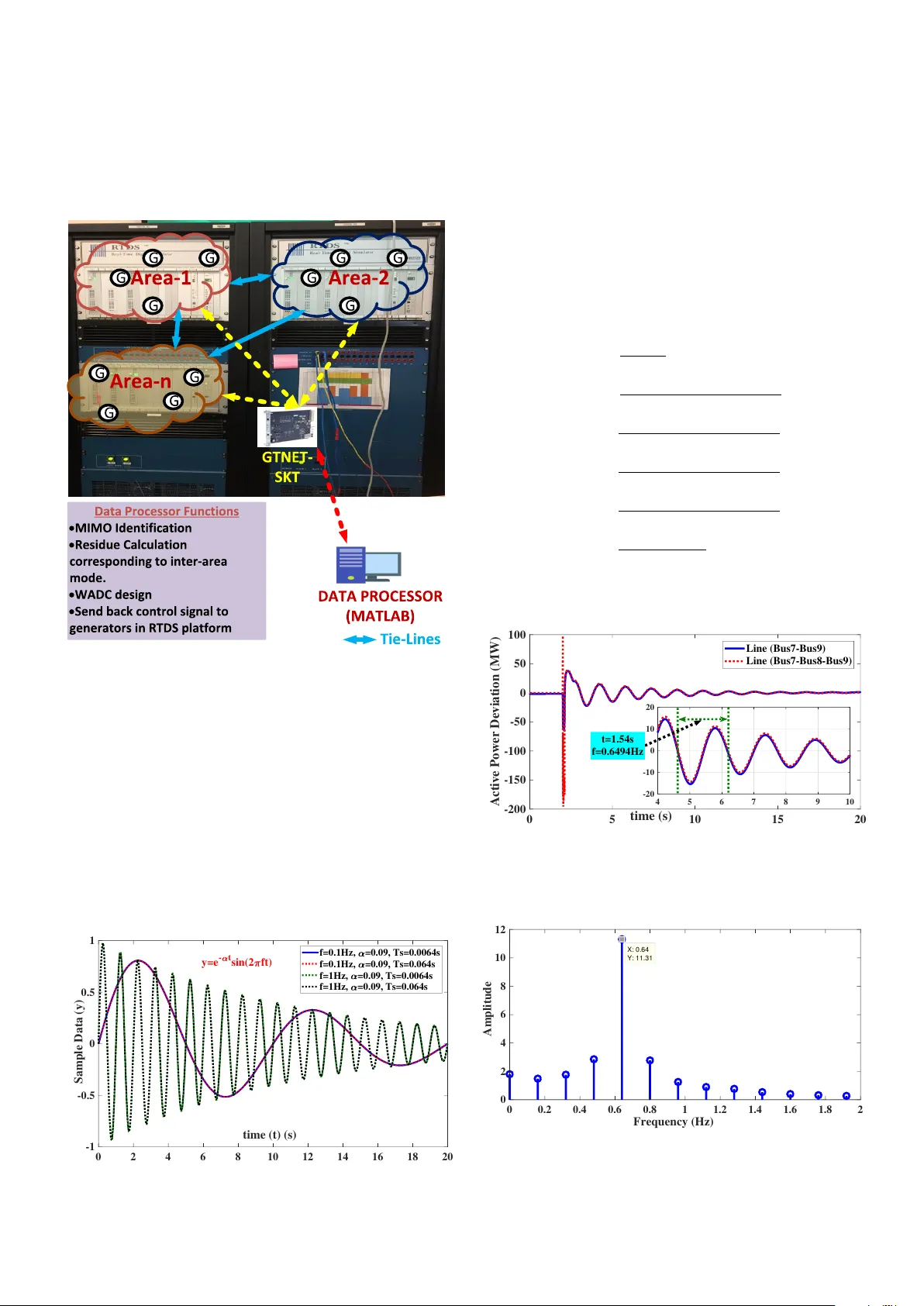
Authors: Abilash Thakallapelli, Sukumar Kamalasadan
Measurement-Based Wide-Area Damping of Inter -Area Oscillations based on MIMO Identification Abilash Thakallapelli 1 , Sukumar Kamalasadan 1 ∗ 1 Electrical and Computer Engineering, UNC Char lotte, Charlotte, USA * E-mail: skamalas@uncc.edu Abstract: Interconnected power grid e xhibits oscillator y response after a disturbance in the system. One such type of oscillations, the inter- area oscillations has the oscillation frequency in the range of 0.1 to 1 Hz. The damping of inter-area oscillations is difficult with local controllers, but it can be achie ved using a Wide Area Damping Controller (W ADC). For effectiv e control, the input to the W ADC should be the most observable signal and the W ADC output should be sent to the most controllab le generator . This paper presents a measurement-based novel algorithm for multi-input-multi-output (MIMO) transfer function identification of the power system based on optimization to estimate such oscillation frequencies. Based on the MIMO transf er function the optimal control loop for W ADC is estimated. The W ADC design is based on the discrete linear quadratic regulator (DLQR) and Kalman filter ing f or damping of inter-area oscillations. Since the MIMO identification is based on actual measurements, the proposed method can accurately monitor changes in the power grid whereas the conventional methods are based on small-signal analysis of a linearized model which does not consider changing operating conditions. The ov erall algorithm is implemented and v alidated on a R TDS/RSCAD R and MA TLAB R real-time co-simulation platf orm using two-area and IEEE 39 bus pow er system models. 1 Introduction The increase in penetration of renewable energy sources and dereg- ulation made the power system to operate near its rated operating limits. Under these circumstances, if there is a disturbance in the system this could affect the po wer system reliability and security . The oscillatory response which arise due to such disturbances have to be damped effecti vely and these oscillations are of two types 1) Local oscillations, and 2) Inter-area oscillations. The local oscilla- tions hav e frequencies greater than 1 Hz and inter-area oscillations frequency lies in the range of 0.1 to 1 Hz [1]. During inter-area oscillations generators in one coherent area swing together against other area generators [2]. In general, such oscillations are suppressed using supplementary control techniques likes po wer system stabi- lizers (PSS) [3], flexible alternating current transmission systems (F A CTS) devices [4] and high-voltage direct current (HVDC) links [5]. Howe ver , such controllers are effecti ve only during local oscilla- tions. As the inter -area oscillations may destabilize the po wer system [6] it should be damped effecti vely . In literature, sev eral methodologies are presented to damp inter- area oscillations using a wide area control loop which is effecti ve to damp an inter-area mode of interest. The wide area control loop is based on the most observable control signal which is input to the wide-area controller and the output of the controller is sent to the most controllable generator . This input/output combination can be estimated based on residue analysis [7–9], combination of residue and relativ e gain array (RGA) method [10], and a joint observability-controllability measure [11, 12]. In all these meth- ods, the control-loop selection is based on linearizing the system at an operating point and analyzing the state space matrices obtained thereafter . If the system operating point changes then the control- loop obtained at a different operating point may not be valid and a new control-loop is to be estimated based on current operating point. Howe ver , linearizing the complex power system model e very time as the operating point changes are tedious and an accurate model of the power system for the current operating point may not be always readily av ailable. T o o vercome the drawbacks of linearization based methods, mea- surement based methods are adapted. In such methods, using the measurements, the MIMO model of the power system can be esti- mated directly without the need for having a detailed model of the power system. Since the changing dynamics/operating points of the system are captured in the measurement data, the MIMO model thus obtained can be used for mode and control loop estimation. The measurement-based methodologies gained interest with the advent of phasor measurement unit (PMUs), and modern communication infrastructure. A mode estimation method based on prony analysis is discussed in [13], howe ver the mutual coupling between differ - ent MIMO loops is not considered in the mode estimation. In [14], a measurement based method is discussed which is based on using simplified power system model and wide-area measurement system (W AMS) data. Howe ver the problems related to the selection of optimal control loop is not addressed here. The use of PMU data for wide-area control of ST A TCOM is addressed in [15], but the effect of mutual coupling during mode estimation and optimal sig- nal selection is not represented. A po wer system model using MIMO identifcation based on auto-regressi ve moving average exogenous (ARMAX) methodology is de veloped in [16] b ut an optimal method for signal selection is not addressed. T o address some of the existing issues, in this paper , a novel mea- surement based MIMO system identification technique for wide-area control considering mutual coupling between dif ferent control loops is presented. The identified MIMO system is used for 1) inter-area oscillation frequency estimation, 2) optimal control loop estimation, and 3) design of wide area controller . T o summarize, the major contributions of this w ork are: • A measurement based MIMO framework considering the mutual coupling of loops for mode estimation. • A method for online optimal control loop selection for W ADC using residue analysis based on measurement data. • An online W ADC based on DLQR and KF techniques which uses the extracted state space matrices from identified MIMO system. • A real-time co-simulation test bed for measurement based MIMO and W ADC considering mutual coupling between different control loops. The rest of the paper is organized as follows: Section II dis- cusses the ov erall architecture and power system division based on pp . 1–12 coherency is discussed. In section III, measurement based MIMO identification is discussed and section IV discusses real-time imple- mentation of MIMO identification. Section V discusses optimal wide area control loop selection and Section VI discusses measure- ment based DLQR and Kalman filter design. Section VII discusses simulation results and Section VIII concludes the paper . 2 Dividing P ower System Based on Coherenc y and Overall Arc hitecture Design of the proposed architecture is based on dividing the power system into areas using coherency grouping and inter tie-line con- nections between areas. First, the active power flow deviation ( ∆ P = P rated − P actual ) through the tie-lines are used as input signal to the W ADC [17]. Then MIMO identification is designed to estimate an optimal control loop to damp the inter-area mode oscillation. Finally , W ADC is designed with a measurement based discrete linear quadratic regulator (DLQR) integrated in kalman fil- tering (KF) technique. Fig. 1 shows the flo wchart of the proposed methodology . The efficac y of the proposed algorithm is verified by implementing on a R TDS/RSCAD and MA TLAB real-time test bed using two-area and IEEE 39 b us power system models. M I M O I d e n t i f i cat i o n ( S e c t io n 3 ) S i g n a l S e l e ct i o n ( S ect i o n 5 ) C o n t r o l l e r D e s i g n a n d A d a p t a t i o n ( S e c t io n 6 ) O f f li n e C o h e r e n c y G r o u p i n g ( S ect i o n 2 ) C o n t r o l S ig n a l P o w e r S y s t e m T i m e D e l a y ( S ect i o n 7 . 1 . 1 a n d 7 . 2 . 3 ) Fig. 1 : Flow-chart of the proposed methodology For grouping of power grid, slow coherency grouping method is considered. Please refer [18] for further details of slow coherency grouping method. This algorithm is implemented on two-area power system (Fig. 2) as well as IEEE 39 bus (Fig. 7) power system models. Further , tie-line po wer flow information is used in deciding the wide- area control action. 2.1 Coherency grouping of two-area system model On applying the slo w coherency grouping method to the two-area power system model, it is found that generators 1 and 2 are in one area and the remaining generators are in other area. T o validate this grouping from the actual response of the system a 3-ph fault is cre- ated at 4s for a duration of 0.05s on bus-8 and generators inter-area dynamics are observed. Fig. 3 shows the speed deviation of genera- tors from its rated speed (i.e 2 π f , where f is fundamental frequency in Hz). It can be seen that generators 1,2 swing against generators 3 and 4. Based on this grouping the test model is divided into two areas (groups) as shown in Fig. 2 and T able 1. From Fig. 2 it can be seen that lines connecting Bus-7 to Bus-8 to Bus-9, and Bus-7 to Bus-9 are the tw o tie-lines. The acti ve po wer flo w deviation of these two lines are represented as ∆ P 1 and ∆ P 2 respectiv ely . Fig. 2 : T wo-area po wer system model 15 15.5 16 16.5 17 17.5 18 18.5 19 19.5 20 time (s) -0.05 0 0.05 Speed Deviation ( ) 1 2 3 4 Fig. 3 : Speed deviation (rad/s) (tw o-area system) 2.2 Coherency grouping of IEEE 39 b us system The IEEE 39 bus system (Fig. 4) coherent groups of generators are obtained using the slow coherency grouping algorithm as shown in T able 1. For validation purpose, a 3-ph fault is created on Bus-14 at 4s for a duration of 0.1s. Fig. 5, Fig. 6, and Fig. 7 shows the speed deviations of generators in groups-1, 2, and 3 respecti vely . From Fig. 4 it can be seen that lines connecting Bus-39 to Bus-1, Bus-39 to Bus-9, Bus-3 to Bus-4, Bus-14 to Bus-15, and Bus-16 to Bus-17 are the tie-lines. The activ e po wer flow deviation of these tie-lines are represented as ∆ P 1 , ∆ P 2 , ∆ P 3 , ∆ P 4 , and ∆ P 5 respectiv ely . 3 Measurement based MIMO Identification Most of the physical world systems are MIMO and traditionally the dynamics of these system are analyzed using linearized model at an operating point and estimating modes and mode shapes from the state space matrices thus obtained after linearization. Howe ver , linearizing a complex system requires accurate model which repre- sents the current operating point of the system, This is often difficult to build. A measurement based MIMO identification can overcome T able 1 Coherency grouping of power system models T est System Slow Coherency T wo Area Group-1: 1,2 Group-2: 3,4 IEEE 39-BUS Group-1: 4,5,6,7 Group-2: 1,8,9 Group-3: 2,3 Group-4: 10 pp . 1–12 2 3 5 4 6 9 8 1 31 39 37 30 3 4 5 6 7 21 22 25 27 34 20 12 13 14 15 16 17 18 7 19 32 10 3 11 10 8 9 33 36 23 35 38 29 28 26 1 2 24 G r o u p - 1 G r o u p - 3 G r o u p - 2 Fig. 4 : 39-bus po wer system model 5 6 7 8 9 10 time (s) -2 -1.5 -1 -0.5 0 Speed Deviation (rad/s) 4 5 6 7 Fig. 5 : Speed Deviation (Group-1) 5 6 7 8 9 10 time (s) -1.5 -1 -0.5 Speed Deviation (rad/s) 1 8 9 Fig. 6 : Speed Deviation (Group-2) modeling accuracy if identified using measured data. Howe ver , the coupling ef fects between dif ferent input/output combinations should be considered while developing an MIMO model. The methodology is discussed using an example in Subsection 3.1. 3.1 MIMO transf er function from state space matrices Consider a system with two inputs, u 1 and u 2 , and two outputs, y 1 and y 2 represented by differential equation [19] as follo ws: y 00 1 + a 1 + y 0 1 + a 0 ( y 1 + y 2 ) = u 1 ( t ) (1) y 0 2 + a 2 ( y 2 − y 1 ) = u 2 ( t ) (2) 5 6 7 8 9 10 time (s) -1.8 -1.6 -1.4 -1.2 -1 -0.8 -0.6 -0.4 Speed Deviation (rad/s) 2 3 Fig. 7 : Speed Deviation (Group-3) where superscripts y 0 and y 00 indicates first and second order dif- ferential equations respectiv ely . In state-space form (1) and (2) giv es: x 1 = y 1 (3) x 4 = y 2 = x 0 3 (4) x 0 1 = y 0 1 = x 2 (5) x 0 2 = − a 1 x 2 − a 0 ( x 1 + x 4 ) + u 1 ( t ) (6) x 0 4 = − a 2 ( x 4 − x 1 ) + u 2 ( t ) (7) Now rearranging (3) to (7) to get state space equations. x 0 = 0 1 0 0 − a 0 − a 1 0 − a 0 0 0 0 1 a 2 0 0 − a 2 | {z } A x + 0 0 1 0 0 0 0 1 | {z } B u 1 u 2 (8) y 1 y 2 = 1 0 0 0 0 0 0 1 | {z } C x (9) Con verting (8) and (9) into transfer function form G ( s ) = C ( sI − A ) − 1 B = G 11 ( s ) G 12 ( s ) G 21 ( s ) G 22 ( s ) (10) where I is the identity matrix and G 11 ( s ) = s + a 2 s 3 + ( a 1 + a 2 ) s 2 + ( a 0 + a 1 a 2 ) s + 2 a 0 a 2 G 12 ( s ) = − a 0 s 3 + ( a 1 + a 2 ) s 2 + ( a 0 + a 1 a 2 ) s + 2 a 0 a 2 G 21 ( s ) = a 2 s 3 + ( a 1 + a 2 ) s 2 + ( a 0 + a 1 a 2 ) s + 2 a 0 a 2 G 22 ( s ) = s 2 + a 1 s + a 0 s 3 + ( a 1 + a 2 ) s 2 + ( a 0 + a 1 a 2 ) s + 2 a 0 a 2 Equation (10) can be represented in discrete time domain by replac- ing s with 2(1 − z − 1 ) T s (1+ z − 1 ) (tustin approximation), where T s is the sampling time. G ( z − 1 ) = G 11 ( z − 1 ) G 12 ( z − 1 ) G 21 ( z − 1 ) G 22 ( z − 1 ) (11) The objective here is to identify the MIMO transfer function as shown in (10) and (11) using the measurement data without having pp . 1–12 any kno wledge of the physical system model. If MIMO identifi- cation is based on different input/output combinations separately , mutual coupling between loops are ignored. Howe ver , if we observe the individual transfer function of (10), it can be seen that all the transfer functions have same denominator coefficients (i.e eigen v al- ues of the system) while numerator coefficients differ . This ensures mutual coupling between loops in MIMO system. So our objective is to formulate a MIMO identification using input/output measure- ment with same denominator coefficients but different numerator coefficients. 3.2 Measurement based MIMO identification considering mutual coupling For measurement based MIMO identification the input data u p is the voltage reference to the exciter of the synchronous machine and the output is the tie-line active power deviation, ∆ P m . The input/output measurement channel is as illustrated in Fig. 8. The real-life sys- tem and EMT based real-time simulator is in discrete-domain, so the MIMO formulation of the power system is also modeled in discrete time domain with p inputs and m outputs as represented in (12). The individual transfer function corresponding to each input/output loop is estimated using the proposed methodology for MIMO identifica- tion considering the mutual coupling between different loops. This can be written as G e n e ra t o r P S S W AD C + + + - A V R + E X C V r e f V t ( T e r mi n a l V o l t a g e ) Δ ω u p s s Δ P ( m o s t o b s e r v a b l e ) I n p u t Si gn a l ( u p ) N e t w ork Δ P m Fig. 8 : Input and output measurements ∆ P ( z − 1 ) = G ( z − 1 ) U ( z − 1 ) (12) where ∆ P ( z − 1 ) = ∆ P 1 ( z − 1 ) . . ∆ P m ( z − 1 ) , U ( z − 1 ) = u 1 ( z − 1 ) . . u p ( z − 1 ) G ( z − 1 ) = G 11 ( z − 1 ) . . G 1 p ( z − 1 ) . . . . . . . . G m 1 ( z − 1 ) . . G mp ( z − 1 ) and G mp ( z − 1 ) = ∆ P m ( z − 1 ) u p ( z − 1 ) = b h 0 + b h 1 z − 1 + ... + b h k z − k 1 + a 1 z − 1 + a 2 z − 2 + ... + a k z − k (13) where u p and ∆ P m are the input and output signal data, h is the element number in matrix, and k is the order of transfer function. It can be seen from (13) that for all transfer functions the denom- inator coefficients are same but numerator coefficients differ . This ensures that mutual coupling effect is taken into account. The steps for MIMO transfer function identification is as follows: 3.2.1 Step-1: The equation (12) is rewritten for N observation window length as sho wn in (14). X h H is = X h N um b h 0 . . . b h k + X h Den a 1 . . a k (14) where X h H is = ∆ P 1 ( z − 1 ) . . ∆ P m ( z − 1 ) X h N um = u p ( z − 1) . u p ( z − k ) . . . . . . u p ( z − N ) . u p ( z − N + 1 − k ) X h Den = ∆ P m ( z − 1) . ∆ P m ( z − k ) . . . . . . ∆ P m ( z − N ) . ∆ P m ( z − N + 1 − k ) 3.2.2 Step-2: For all input/output loops, concatenate X h H is and is represented as (15) X 1 H is X 2 H is . X h H is | {z } X H = X 1 N um X 2 N um . X h N um b 1 0 . . . b 1 k b 2 0 . . . b 2 k . . . b h 0 . . . b h k | {z } X N + X 1 Den X 2 Den . X h Den a 1 . . a k | {z } X D (15) 3.2.3 Step-3: The numerator and denominator coefficients are estimated using an optimization algorithm where the optimization function is represented as (16) minimize k X H − [ X N + X D ] k (16) Initial conditions for the numerator ( b h 0 , b h 1 ...b h k ) and denominator ( a 1 , a 2 ...a k ) coefficients are estimated from a least squares tech- nique formulated as constrained nonlinear multi variable function. For this the MA TLAB based f mincon function is used to solve the unknowns. 4 Real-time implementation of MIMO identification The proposed MIMO identification of the power system is imple- mented on a R TDS/RSCAD and MA TLAB co-simulation test bed as shown in Fig. 9. The power system is modeled in R TDS/RSCAD and the MIMO identification algorithm is implemented in MA TLAB. The real-time measured data from the digital simulator is processed through an Ethernet based ocket connection [20]. The data receiv ed pp . 1–12 is then processed for MIMO identification. Also the identified trans- fer function is used to estimate an optimal control loop. The control signel is then send back to the power system model in the digital sim- ulator . Since this approach is implemented using R TDS, the process exactly emulates the real-life scenario. Thus the designed controller can be tested using this co-simulation platform before implementing in field. Fig. 9 : Real-time experimental setup 4.1 Data Criter ia The proposed algorithm is first validated on the two-area power system model (Fig. 2). The measurement data u p and ∆ P m of all generators are extracted with a sampling time ( T s ) of 0.0032s. The data-set is then down-sampled by a factor 10 so that the new sampling time will be 0.032s. The new sampling time after down-sampling is used to estimate inter-area modes. The inter-area frequency range is between 0.1 to 1Hz so for a successful estimation of inter-area frequency a window length of two cycles of the lowest frequency is considered as sho wn in Fig. 10. 0 2 4 6 8 10 12 14 16 18 20 time (t) (s) -1 -0.5 0 0.5 1 Sample Data (y) f=0.1Hz, =0.09, Ts=0.0064s f=0.1Hz, =0.09, Ts=0.064s f=1Hz, =0.09, Ts=0.0064s f=1Hz, =0.09, Ts=0.064s y=e - t sin(2 ft) Fig. 10 : Data requirement 4.2 MIMO Identification two-area system T o validate the effectiv eness of the proposed MIMO identification algorithm in estimating the inter-area modes, a 3-ph fault is cre- ated on Bus-8 at 4s for a duration of 0.05s. The speed deviation after the fault is shown in Fig. 11. From visual inspection, It can be seen that the approximate frequency of oscillation is 0.6494Hz. From fast fourier transform (FFT) algorithm on ∆ P 1 data, it can be seen that the frequency is 0.64Hz as well (see Fig. 12). The estimated transfer function between ∆ P 1 (Bus-7 to Bus-8 to Bus-9) and u 4 (Generator-4) is shown in (19). Using the transfer function, the frequency obtained from the proposed algorithm considering mutual coupling is 0.6362Hz. T able 2 shows the inter-area mode comparison. G 14 ( z ) = ∆ P 1 ( z ) u 4 ( z ) = 59 . 2665 − 6 . 7181 i 1 − (0 . 9835 + 0 . 1257 i ) z − 1 + 59 . 2665 + 6 . 7181 i 1 − (0 . 9835 − 0 . 1257 i ) z − 1 + − 0 . 2852 + 38 . 1373 i 1 − (0 . 9300 + 0 . 2484 i ) z − 1 + − 0 . 2852 − 38 . 1373 i 1 − (0 . 9300 − 0 . 2484 i ) z − 1 + − 89 . 7368 1 − 0 . 9961 z − 1 − 28 . 9939 (17) 0 5 10 15 20 time (s) -200 -150 -100 -50 0 50 100 Active Power Deviation (MW) Line (Bus7-Bus9) Line (Bus7-Bus8-Bus9) 4 5 6 7 8 9 10 -20 -10 0 10 20 t=1.54s f=0.6494Hz Fig. 11 : T ie-lines activ e power de viation ( ∆ P 1 ) 0 0.2 0.4 0.6 0.8 1 1.2 1.4 1.6 1.8 2 Frequency (Hz) 0 2 4 6 8 10 12 Amplitude X: 0.64 Y: 11.31 Fig. 12 : FFT analysis of ∆ P 1 pp . 1–12 T able 2 Inter-area mode compar ison T est System MIMO Identification FFT T wo Area 0.6362Hz 0.64Hz IEEE 39-BUS Case-1: 0.6077Hz Case-1: 0.599Hz Case-2: 0.6098Hz Case-2: 0.6024Hz 4.3 MIMO Identification of 39-bus system In order to sho w the scalability and usefulness of the algorithm, case studies with multiple disturbance with multiple machines are ev alu- ated using IEEE 39 bus system. T wo sequential disturbance cases at different locations as sho wn in Fig. 13 are simulated. 4.3.1 Case:1: In this case a 3-ph fault is created at 14s for a duration of 0.1s on bus-14. From T able 2 it can be seen that, using the proposed method, estimated inter-area frequency is 0.6077Hz whereas from FFT analysis of ∆ P 1 (Bus-39 to Bus-1) data the inter-area frequenc y obtained is 0.599Hz (Fig. 14). 4.3.2 Case:2: In this case a 3-ph fault is created at 39.5s for a duration of 0.1s on bus-19. From T able 2 it can be seen that from the proposed method the estimated inter-area frequency is 0.6098Hz whereas from FFT analysis of ∆ P 1 (Bus-39 to Bus-1) the inter- area frequency obtained is 0.6024Hz (Fig. 15). This pro ves that the proposed architecture can accurately represents the oscillation frequency . 5 Optimal Wide Area Control Loop Selection After estimating the inter-area mode the objective is to damp that oscillation using W ADC. Ho we ver , in the MIMO power system model there are different input/output control loop combinations, it is important to estimate the most optimal control loop with which we can damp inter-area oscillations. This can be achieved by analyzing residues of the identified MIMO transfer functions corresponding to inter-area modes of interest [21]. For this, (13) is con verted to con- tinuous time domain format and rewritten in partial fraction form as shown in (18). G mp ( s ) = ∆ ω m ( s ) u p ( s ) = r mp (1) s − p 1 + r mp (2) s − p 2 + .. + r mp ( j ) s − p j + k mp ( s ) (18) The transfer function between ∆ P 1 (Bus-7 to Bus-8 to Bus-9) and u 4 (Generator-4) using the proposed algorithm in continuous domain can be represented as (19). G 14 ( z ) = ∆ P 1 ( s ) u 4 ( s ) = − 15 . 127 + 1211 . 8 i s − ( − 1 . 2121 + 8 . 2017 i ) + − 15 . 127 − 1211 . 8 i s − ( − 1 . 2121 − 8 . 2017 i ) + 1859 . 7 − 209 . 77 i s − ( − 0 . 26881 + 3 . 9774 i ) + 1859 . 7 + 209 . 77 i s − ( − 0 . 26881 − 3 . 9774 i ) + − 2804 . 3 s − ( − 0 . 12207) − 10 . 142 (19) where p and r mp are the poles and residues of the transfer function G mp ( s ) . The residue ( r mp ( j ) ) corresponding to inter-area mode ( p j ) giv es the information of the optimal control loop. For a mode p j , the value of residue giv es how controllable is the output ∆ P m and how observ able is the input u p , meaning how strong is the con- trol loop to damp oscillations. It can be concluded that the control loop which has larger residue is the optimal loop. 5.1 Identifying the optimal control loop f or two-area system From T able 2 it can be seen that the dominant inter-area mode for two-area po wer system model is 0.6362Hz. The residue analysis cor- responding to the inter-area mode of frequency 0.6362Hz is shown in T able 3. From T able 3 it can be seen that the maximum value of residue is for ∆ P 1 → u 3 loop which is the most optimal. From this, generator-3 is the most controllable and the activ e power deviation ∆ P 1 is the most observable signal. T able 3 Optimal wide area control loop based on normalized residue analysis output/input u 1 u 2 u 3 u 4 ∆ P 1 (Bus-7 to Bus-8 to Bus-9) 0.3335 0.42875 1 0.44531 ∆ P 2 (Bus-7 to Bus-9) 0.32973 0.42015 0.99597 0.47881 5.2 Identifying the optimal control loop f or 39 bus system For 39 b us system, dif ferent cases are analyzed as discussed in Section 4.3.1 and 4.3.2 to illustrate how changes in operating condi- tions affect the inter-area modes and corresponding optimal control loops. 5.2.1 Case: 1: From T able 2 dominant inter-area mode for 39 bus system, case-1 is 0.6077Hz. The residue analysis corresponding to inter-area mode of frequency 0.6077Hz for top three control loops are shown in T able 4. From T able 4 it can be seen that generator-1, generator-8, and generator -9 are the most controllable and the corre- sponding observable signals are ∆ P 2 , ∆ P 1 , and ∆ P 2 respectiv ely . T able 4 Optimal control loop for IEEE 39-bus (F ault on Bus-14) Control Loop Residue ∆ P 2 (Bus-39 to Bus-9) to u 1 1.0 ∆ P 1 (Bus-39 to Bus-1) to u 8 0.8051 ∆ P 2 (Bus-39 to Bus-9) to u 9 0.7350 5.2.2 Case: 2: From T able 2 dominant inter-area mode for 39 bus system, case-2 is 0.6098Hz. The residue analysis corresponding to inter-area mode of frequency 0.6098Hz for top three control loops are shown in T able 5. From T able 5 it can be seen that generator-10, generator-1, and generator -8 are the most controllable and the corre- sponding observable signals are ∆ P 5 , ∆ P 5 , and ∆ P 1 respectiv ely . T able 5 Optimal control loop for IEEE 39-bus (F ault on Bus-19) Control Loop Residue ∆ P 5 (Bus-16 to Bus-17) to u 10 1.0 ∆ P 5 (Bus-16 to Bus-17) to u 1 0.6993 ∆ P 1 (Bus-39 to Bus-1) to u 8 0.4738 6 Measurement based DLQR and Kalman filter design The W ADC design is based on DLQR and KF . The W ADC design architecture is as shown in Fig. 16. pp . 1–12 0 10 20 30 40 50 60 70 time (s) -300 -200 -100 0 100 200 300 400 Active Power Deviation (MW) P 1 P 2 P 3 P 4 P 5 Case: 1 Frequency: 0.6077Hz MIMO Order: 7 Case:2 Frequency: 0.6098 MIMO Order: 7 Fig. 13 : 39 bus tie-line acti ve po wer de viation 0 0.5 1 1.5 2 Frequency (Hz) 0 20 40 60 Amplitude X: 0.599 Y: 69.42 Fig. 14 : FFT analysis of ∆ P 1 (Case:1) 0 0.5 1 1.5 2 Frequency (Hz) 0 20 40 60 Amplitude X: 0.6024 Y: 63.31 Fig. 15 : FFT analysis of ∆ P 1 (Case:2) 6.1 Discrete-time linear quadratic regulator The DLQR based controller uses state space matrices correspond- ing to optimal control loop for calculating the control gain. For this the discrete state space model is extracted from the MIMO transfer functions (13) and represented as follows: x k +1 = A k x k + B k u k y k = C k x k + D k u k (20) where A , B , C , and D are the state, input, output, and feed forward matrices respectively . The objectiv e of the DLQR is to minimize M I M O I d e n ti f i c a t i o n D L Q R C o n t r o l l e r E q n s ( 21 a - 21 d ) K - 1 K a l m a n S t a t e E s t i m a t i on E q n s ( 22 - 26 ) [ x ] u = - K [ x ] E q n . 21 b A , B , C , D ( E q n . 20 ) A , B , C , D ( E q n . 20 ) P ow e r S y s t e m W A DC T o Mo s t C o n t r o l l a b l e G e n e r a t or Fig. 16 : W ADC architecture the cost of the objective function represented as (21a), where R = ρI ( ρ > 0) , Q = C T k C k are the weight matrices and N is the num- ber of samples. The cost function can be minimized by calculating optimal control gain K by solving (21c)-(21d). The P in (21c) is the solution of the discrete algebraic Ricatti equations represented as (21d). The optimal control signal is represented as (21b) [22] which is sent to most controllable generator estimated from residue analysis. J = N X k =0 ( x T k Qx k + u T k Ru k ) (21a) u k = − K k x k (21b) K k = ( R + B T k P k +1 B k ) − 1 B T k P k +1 A k (21c) P k − 1 = Q + A T k P k A k − A T k P k B k ( R + B T k P k B k ) − 1 B T k P k A k (21d) T able 6 shows the estimated optimal control gains for two-area system. T able 7 and T able 8 shows the optimal control gains for 39- bus system Case 1 and 2 respecti vely . pp . 1–12 T able 6 Estimated LQR gains ( K ) for two-area system Control Loop Gain (K) ∆ P 1 to u 3 [0.089446 -0.1349 0.073803 -0.033455 0.019523] T able 7 Estimated LQR gains ( K ) for IEEE 39 b us system (Case:1) Control Loop Gain (K) ∆ P 2 to u 1 [0.0041 -0.0065 -0.0029 0.0295 -0.0407 0.0233 -0.0190] ∆ P 1 to u 8 [-0.0467 0.1225 -0.2635 0.2954 -0.1783 0.0519 -0.0188] ∆ P 2 to u 9 [-0.0296 0.0884 -0.2031 0.2372 -0.1477 0.0448 -0.0188] T able 8 Estimated LQR gains ( K ) for IEEE 39 b us system (Case:2) Control Loop Gain (K) ∆ P 5 to u 10 [-0.0919 0.3275 -0.4145 0.2566 -0.1636 0.0935 -0.0207] ∆ P 5 to u 1 [-0.0858 0.3297 -0.4227 0.2606 -0.1645 0.0931 -0.0207] ∆ P 1 to u 8 [-0.0445 0.1546 -0.1984 0.1249 -0.0807 0.0465 -0.0104] 6.2 Kalman filtering based state estimation The optimal control signal in (21b) is the product of the optimal control gain and states of the system corresponding to optimal con- trol loop. Here, KF technique is adapted to estimate the states of the system. The state space model as shown in (20) is used to estimate the states. The predictor step and co-v ariance calculation is giv en by (22) and (23) respectiv ely . x k +1 = A k x k + B k u k (22) L k = A k L k − 1 A T k + Q k (23) where Q and L are co-variance of noise and state vector estimate respectiv ely . The Kalman gain factor ( G ) is estimated as sho wn in (24) G k = L k H T k ( H k L k H T k + R k ) − 1 (24) where R and H are co-variance of measurement noise and and the observation matrix respecti vely . The corrector step is represented as shown in (25) and (26). x k = x k +1 + G k ( z − H xk + 1) (25) L k = L k +1 − K k H k L k +1 (26) Further details of kalman filtering based state estimation are reported in [23]. 7 Simulation Results The output of W ADC is sent to the most controllable generator as shown in Fig. 16. Implementation results on two-area and IEEE 39 bus system models considering various disturbances are illustrated next. 7.1 Simulation results of two-area system The wide area control loop for two-area system is as shown in Fig. 17. Fig. 18 sho ws the speed de viation of generator 2 with and without W ADC. Fig. 19 shows the speed deviation of generator 4 with and without W ADC. Fig. 20 shows the tie-line acti ve power deviation ∆ P 1 . Fig. 21 shows the W ADC output sent to generator 3. From the abov e figures it can be seen that the with the proposed approach the oscillations are damped effecti vely . T able 9 shows the comparison of performance metrics with and without W ADC. The speed devia- tion value for generator -2 without W ADC at 11s after disturbance is 0.01773 whereas with W ADC the value is 0.0038. This indicates that there is 78.68% reduction in oscillation magnitude. In the same w ay for generator-4 there is 72.60% reduction in oscillation magnitude. Further area-under the curve for the absolute value of oscillations is analyzed as shown in T able 10 and found that for generator-2 the area under the curve is 66% less with W ADC and for generator-4 it is 56% less. The area under the curve for tie-line po wer flow de viation is 51% less with W ADC. T able 9 Perf ormance metr ics for tw o-area system V ar iable Without W ADC With W ADC P eak ∆ ω 2 at 15s (Fig. 18) 0.01773 0.0038 P eak ∆ ω 4 at 14.25s (Fig. 20) 0.0413 0.0113 T able 10 Area under the cur ve f or two-area system V ar iable Without W ADC With W ADC ∆ ω 2 (Fig. 18) 0.4817 0.1638 ∆ ω 4 (Fig. 19) 0.6959 0.3012 ∆ P 1 (Fig. 20) 11.739 5.75 WAD C Fig. 17 : Optimal control loop for two-area system 0 2 4 6 8 10 12 14 16 18 20 time (s) -0.4 -0.2 0 0.2 0.4 0.6 0.8 1 1.2 Speed Deviation ( 2 ) With WADC Without WADC 10 11 12 13 14 15 16 17 18 19 20 -0.02 0 0.02 0.04 0.06 Fig. 18 : Generator-2 speed de viation (rad/s) 7.1.1 Eff ect of time-delay on two-area system control: T o study the effect of time-delay on the control, an intentional time- delay is created in addition to the inherent time delay . The inherent time delay for the two-area system case is 0.15s. The intentional time delay is created in the control loop at the time delay block as shown in Fig. 1. Initially , a time delay of 1 ms is created which is pp . 1–12 0 2 4 6 8 10 12 14 16 18 20 time (s) -0.4 -0.2 0 0.2 0.4 0.6 0.8 1 Speed Deviation ( 4 ) With WADC Without WADC 10 12 14 16 18 20 -0.04 -0.02 0 0.02 0.04 0.06 Fig. 19 : Generator-4 speed de viation (rad/s) 0 5 10 15 20 time (s) -80 -60 -40 -20 0 20 40 Active Power Deviation (MW) With WADC Without WADC 10 11 12 13 14 15 16 17 18 19 20 -4 -2 0 2 4 Fig. 20 : T ie-line activ e power flo w de viation ( ∆ P 1 ) 0 2 4 6 8 10 12 14 16 18 20 time (s) -0.08 -0.06 -0.04 -0.02 0 0.02 0.04 WADC Control Signal G3 Fig. 21 : W ADC output signal further increased up to 500 ms . It can be observed from Fig. 22 that for an extra time delay of 300 ms the controller performance started to deteriorate and as the time delay is increased further the system is driv en into unstable mode. F or quantitativ e analysis, relativ e error is calculated using (27). r elativ e er ror = ∆ P ref − ∆ P delay 2 ∆ P ref 2 (27) where ∆ P ref represents the response with inherent time delay and ∆ P delay represents the response with intentional time delay . T able 11 shows the relative error comparison for different time delays. It can be seen that the error increases as the time delay increases. 7.2 Simulation results of 39 b us system For this system two cases are analyzed for dif ferent disturbances. 0 5 10 15 20 time (s) -80 -60 -40 -20 0 20 40 Active Power Deviation (MW) Inherent time delay only Inherent time delay + 1ms Inherent time delay + 50ms Inherent time delay + 300ms Inherent time delay + 500ms Fig. 22 : T ie-line activ e power flo w de viation (∆ P 1 ) T able 11 Relative error for v arious time delays (two-area system) Time Delay Relative Error 1ms 0.029319 50ms 0.42091 300ms 0.52231 500ms 1.7834 7.2.1 Case:1: For the same disturbance scenario as discussed in Section 4.3.1, Fig. 23 and Fig. 24 shows the activ e power devi- ations ∆ P 2 , and ∆ P 4 respectiv ely . Fig. 25, and Fig. 26 shows the speed deviations of generator 4, and 10 with and without W ADC respectiv ely . Fig. 27 shows the W ADC output sent to most con- trollable generator . From the above figures it can be seen that with the proposed approach oscillations are damped effecti vely . The area under the curve for absolute value of speed deviations are analyzed as shown in T able 12 and it is found that the area under the curve is reduced by 59%, and 60.56% with W ADC for generators 4, and 10 respectiv ely . T able 12 Area under the cur ve metric (39 bus system case:1) V ar iable Without W ADC With W ADC ∆ ω 4 (Fig. 25) 6.3374 2.7498 ∆ ω 10 (Fig. 26) 6.3081 2.4878 14 16 18 20 22 24 26 28 30 time (s) -300 -200 -100 0 100 200 300 Active Power Deviation (MW) With WADC Without WADC Fig. 23 : T ie-line acti ve po wer flo w de viation ( ∆ P 2 (Bus-39 to Bus-9)) 7.2.2 Case:2: For the same disturbance scenario as discussed in Section 4.3.2. Fig. 29 and Fig. 30 sho ws the acti ve po wer deviations ∆ P 2 , and ∆ P 4 respectiv ely . Fig. 31, and Fig. 32 shows the speed deviations of generator 7, and 10 with and without W ADC respec- tiv ely . Fig. 33 sho ws the W ADC output sent to most controllable pp . 1–12 14 16 18 20 22 24 26 28 30 time (s) -150 -100 -50 0 50 100 150 200 Active Power Deviation (MW) With WADC Without WADC Fig. 24 : T ie-line acti ve po wer flo w de viation ( ∆ P 4 (Bus-14 to Bus-15)) 15 20 25 30 time (s) -0.5 0 0.5 1 1.5 Speed Deviation ( 4 ) With WADC Without WADC Fig. 25 : Generator-4 speed de viation (rad/s) 15 20 25 30 time (s) -0.5 0 0.5 1 Speed Deviation ( 10 ) With WADC Without WADC Fig. 26 : Generator-10 speed de viation (rad/s) generator . From the above mentioned figures it can be seen that the with the proposed approach the oscillations are damped effecti vely . The area under the curve for absolute value of speed deviations are analyzed as sho wn in T able 13 and it is found that the area under the curve is reduced by 54%, and 56% with W ADC for generators 7, and 10 respectiv ely . 7.2.3 Eff ect of time-delay on 39 bus system control: The inherent time delay for the 39 bus system case is 0.23s. The inten- tional time delay is created in the control loop at the time delay block as shown in Fig. 1. Initially , a time delay of 1 ms is created and increased up to 800 ms . It can be observed from Fig. 28 and 14 16 18 20 22 24 26 28 30 time (s) -0.15 -0.1 -0.05 0 0.05 0.1 0.15 WADC Control Signal G1 G8 G9 Fig. 27 : W ADC output signal 14 16 18 20 22 24 26 28 30 time (s) -300 -200 -100 0 100 200 300 Active Power Deviation (MW) Inherent time delay only Inherent time delay+1ms Inherent time delay+50ms Inherent time delay+500ms Inherent time delay+800ms Fig. 28 : T ie-line activ e power flo w de viation (∆ P 1 ) T able 13 Area under the cur ve metric (39 bus system case:2) V ar iable Without W ADC With W ADC ∆ ω 7 (Fig. 31) 3.746 1.7233 ∆ ω 10 (Fig. 32) 3.5383 1.5359 40 45 50 55 time (s) -300 -200 -100 0 100 200 300 Active Power Deviation (MW) With WADC Without WADC Fig. 29 : T ie-line acti ve po wer flo w de viation ( ∆ P 2 (Bus-39 to Bus-9)) Fig. 34 that for an extra time delay of 500 ms the controller per- formance started to deteriorate and as the time delay is increased further the system oscillations also increased. T able 14 shows the relativ e error comparison for 39 bus system for various time delays calculated using (27). In this case also the relative error increases as the time delay increases. pp . 1–12 40 45 50 55 time (s) -150 -100 -50 0 50 100 Active Power Deviation (MW) With WADC Without WADC Fig. 30 : T ie-line acti ve po wer flo w de viation ( ∆ P 4 (Bus-14 to Bus-15)) 40 45 50 55 time (s) -0.5 0 0.5 1 Speed Deviation ( 7 ) With WADC Without WADC Fig. 31 : Generator-7 speed de viation (rad/s) 40 45 50 55 time (s) -0.5 0 0.5 1 1.5 Speed Deviation ( 10 ) With WADC Without WADC Fig. 32 : Generator-10 speed de viation (rad/s) 8 Conclusion The proposed method for measurement based wide area damping of inter-area oscillations based on MIMO identification ov ercome the drawbacks of earlier linearization based methods reported in litera- ture. In this approach, initially MIMO system transfer functions are identified, then the inter-area modes are estimated using the MIMO transfer functions. The optimal control loop required for W ADC is estimated through residues corresponding to the inter-area mode of interest. Finally , the W ADC is design based on a combination of DLQR and Kalman filtering algorithms. The effectiv eness of the proposed algorithm is verified by implementing on two-area and 40 45 50 55 time (s) -0.15 -0.1 -0.05 0 0.05 0.1 0.15 WADC Control Signal G1 G8 G10 Fig. 33 : W ADC output signal 40 45 50 55 time (s) -300 -200 -100 0 100 200 300 Active Power Deviation (MW) Inherent time delay only Inherent time delay+1ms Inherent time delay+50ms Inherent time delay+500ms Inherent time delay+800ms Fig. 34 : T ie-line activ e power flo w de viation (∆ P 1 ) T able 14 Relative error for v arious time delays (39 bus system) Case:1 Case:2 Time Delay Relative Error Relative Error 1ms 0.0526 0.0376 50ms 0.1469 0.1311 300ms 0.4979 0.3216 500ms 0.6429 0.6418 IEEE 39 bus power system models on R TDS/RSCAD and MA TLAB based real-time co-simulation platform. In the future, framework to mitigate time-delay ef fects on the control action will be addressed. 9 References 1 Klein, M., Rogers, G.J., Kundur , P .: ‘ A fundamental study of inter-area oscillations in po wer systems’, IEEE Tr ansactions on P ower Systems , 1991, 6 , (3), pp. 914–921 2 Chow , J.H.: ‘Power System Coherency and Model Reduction’. Power Electronics and Power Systems. (Springer New Y ork, 2014). A vailable from: https:// books.google.com/books?id=HGnABAAAQBAJ 3 Rogers, G.: ‘Power System Oscillations’. Power Electronics and Power Sys- tems. (Springer US, 2012). A vailable from: https://books.google.com/ books?id=xOTTBwAAQBAJ 4 Y ao, W ., Jiang, L., W en, J., Wu, Q.H., Cheng, S.: ‘W ide-area damping controller of facts devices for inter -area oscillations considering communication time delays’, IEEE Tr ansactions on P ower Systems , 2014, 29 , (1), pp. 318–329 5 Azad, S.P ., Iravani, R., T ate, J.E.: ‘Damping inter-area oscillations based on a model predictive control (mpc) hvdc supplementary controller’, IEEE Tr ansac- tions on P ower Systems , 2013, 28 , (3), pp. 3174–3183 6 Pal, B., Chaudhuri, B.: ‘Robust Control in Power Systems’. Power Electronics and Power Systems. (Springer US, 2006). A vailable from: https://books. google.com/books?id=UXh1o196- McC 7 Juanjuan, W ., Chuang, F ., Y ao, Z.: ‘Design of W AMS-based multiple HVDC damping control system’, IEEE Tr ans Smart Grid , 2008, 2 , pp. 572–581 8 Li, Y ., Rehtanz, C., Ruberg, S., Luo, L., Cao, Y .: ‘Wide-area robust coordina- tion approach of HVDC and F ACTS controllers for damping multiple inter-area oscillations’, IEEE Tr ans P ower Del , 2012, 27 , pp. 1096–1105 9 Kunjumuhammed, L.P ., Singh, R., Pal, B.C.: ‘R obust signal selection for damping of inter-area oscillations’, Pr oc IET Gener Tr ansm Distrib , 2012, 6 , pp. 404–416 pp . 1–12 10 Li, Y ., Rehtanz, C., Ruberg, S., Luo, L., Cao, Y .: ‘ Assessment and choice of input signals for multiple HVDC and F ACTS wide-area damping controllers’, IEEE T rans P ower Syst , 2012, 27 , pp. 1969–1977 11 Dominguez.Garcia, J.L., Ugalde.Loo, C.E., Binachi, F ., GomisBellmunt, O.: ‘Input and output signal selection for damping of power system oscillations using wind power plants’, Int J Electr P ower Energy Syst , 2014, 58 , pp. 75–84 12 Nguyen.Duc, H., Dessaint, L., Okou, A.F ., Kamwa, I. ‘Selection of input/output signals for wide area control loops’. In: Proc. IEEE Power & Energy Society General Meeting. (, 2010. pp. 1–7 13 Zacharia, L., Hadjidemetriou, L., Kyriakides, E.: ‘Integration of renewables into the wide area control scheme for damping power oscillations’, IEEE Tr ans P ower Syst , 2018, PP , pp. 1–9 14 Pradhan, V ., Kulkarni, A.M., Khaparde, S.A.: ‘ A model-free approach for emer- gency damping control using wide area measurements’, IEEE T rans P ower Syst , 2018, PP , pp. 1–11 15 Musleh, A.S., Muyeen, S.M., Al.Durra, A., Kamwa, I.: ‘T esting and validation of wide-area control of statcom using real-time digital simulator with hybrid hilâ ˘ A ¸ Ssil configuration’, IET Gener T ransm Distrib , 2017, 11 , pp. 3039–3049 16 Liu, H., Zhu, L., Pan, Z., Bai, F ., Liu, Y ., Liu, Y ., et al.: ‘ Armax-based trans- fer function model identification using wide-area measurement for adaptive and coordinated damping control’, IEEE Tr ansactions on Smart Grid , 2017, 8 , (3), pp. 1105–1115 17 B..B..Padhy , S.C.S., V erma, N.K.: ‘ A coherency-based approach for signal selec- tion for wide area stabilizing control in power systems’, IEEE Systems Journal , 2013, 7 , (4), pp. 807–816 18 Sanchez . Gasca, J.J., Chow , J.H.: ‘Performance comparison of three identification methods for the analysis of electromechanical oscillations’, IEEE Tr ans on P ower Syst , 1999, 14 , (3), pp. 995–1002 19 ‘Control systems/mimo systems’. (, . A vailable from: https://en. wikibooks.org/wiki/Control_Systems/MIMO_Systems 20 ‘Gtnetx2: the powerful ne w network interface card’. (, . A vailable from: https://www.rtds.com/ gtnetx2- the- powerful- new- network- interface- card/ 21 Thakallapelli, A., Hossain, S.J., Kamalasadan, S. ‘Coherency based online wide area control of wind integrated power grid’. In: 2016 IEEE International Con- ference on Power Electronics, Drives and Energy Systems (PEDES). (, 2016. pp. 1–6 22 Zhang, W ., Hu, J., Abate, A.: ‘On the value functions of the discrete-time switched lqr problem’, IEEE Tr ansactions on Automatic Control , 2009, 54 , (11), pp. 2669– 2674 23 Zhang, J., W elch, G., Bishop, G., Huang, Z.: ‘ A two-stage kalman filter approach for robust and real-time power system state estimation’, IEEE Tr ansactions on Sustainable Energy , 2014, 5 , (2), pp. 629–636 pp . 1–12
Original Paper
Loading high-quality paper...
Comments & Academic Discussion
Loading comments...
Leave a Comment