Network Effects on Robustness of Dynamic Systems

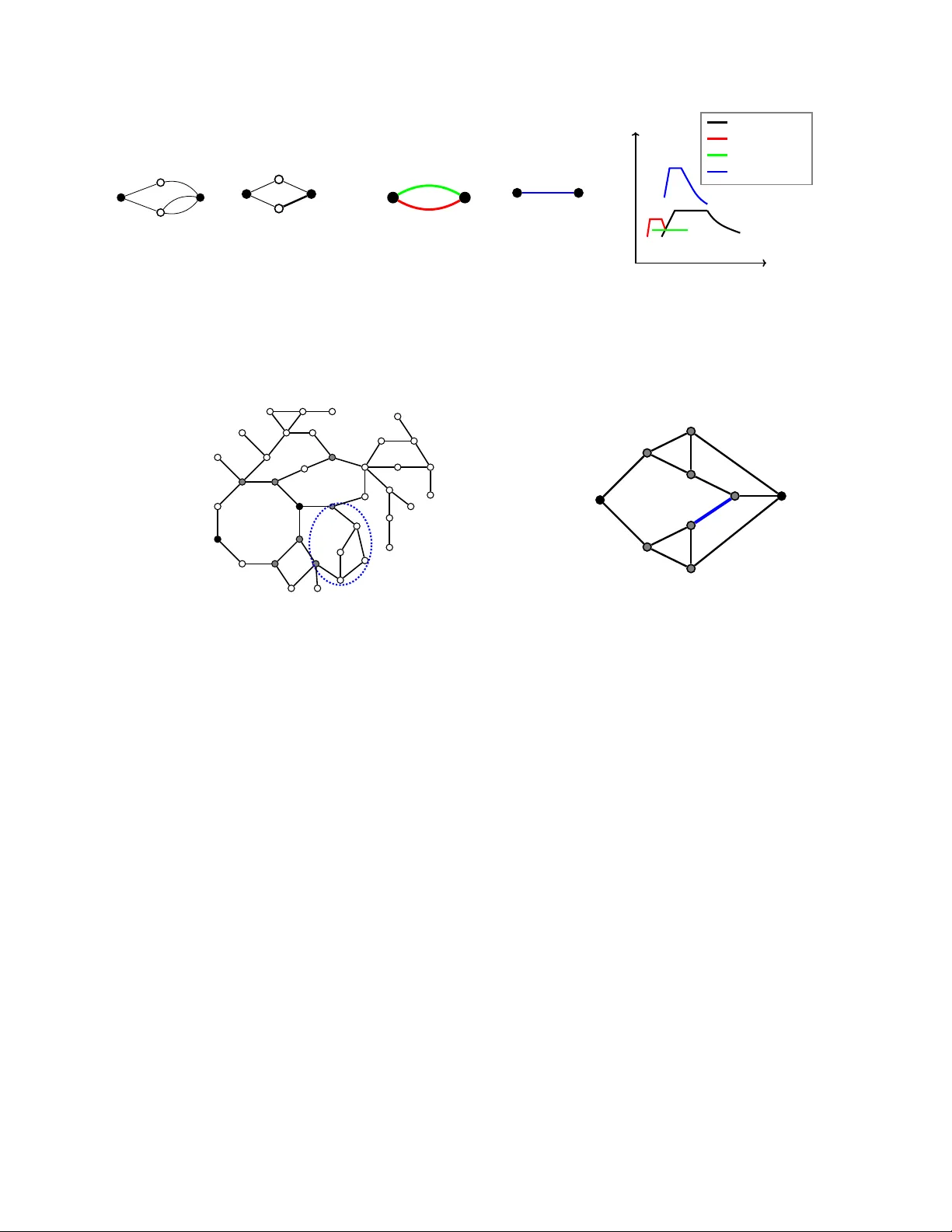
1 Network Ef fects on Rob ustness of Dynamic Systems K etan Savla, Jef f S. Shamma, and Munther A. Dahleh A B S T R AC T W e revie w selected results related to rob ustness of networked systems in ﬁnite and asymptotically large size regimes, under static and dynamical settings. In the static setting, within the frame work of ﬂow over ﬁnite networks, we discuss the effect of physical constraints on rob ustness to loss in link capacities. In the dynamical setting, we revie w se veral settings in which small gain type analysis provides tight robustness guarantees for linear dynamics ov er ﬁnite networks tow ards worst-case and stochastic disturbances. W e also discuss network ﬂow dynamic settings where nonlinear techniques facilitate in understanding the ef fect on robustness of constraints on capacity and information, substituting information with control action, and cascading failure. W e also contrast the latter with a representativ e contagion model. For asymptotically large networks, we discuss the role of network properties in connecting microscopic shocks to emergent macroscopic ﬂuctuations under linear dynamics as well as for economic networks at equilibrium. Through the revie w of these results, the paper aims to achie ve two objectiv es. First, to highlight selected settings in which the role of interconnectivity structure of a network on its robustness is well-understood. Second, to highlight a few additional settings in which existing system theoretic tools give tight robustness guarantees, and which are also appropriate av enues for future network-theoretic in vestigations. I . I N T RO D U C T I O N A N D O V E R V I E W Robustness is the ability of a system to operate effecti vely under a range of different en vironmental conditions or in the face of possible disruptions. What is the impact of incidents on traf ﬁc ﬂo w? Ho w does an energy grid respond to surges in demand? How do supply chain disruptions impact a production economy? Under what conditions can a communication network maintain quality of service? Of course, the issue of robustness is at the heart of control systems and a primary motiv ation for the introduction of feedback in dynamical systems. While the concept of robustness is widely relev ant to multiple domains, an application area of particular impor- tance is networked systems, including physical networks; ﬁnancial, economic and social networks; or networks of people and systems. Indeed, tremendous advances in communication, computation, and sensing have led to renewed interest in networked systems, in that new technologies are introducing unprecedented interdependencies between people, devices, and infrastructure. Ketan Savla is with the Univ ersity of Southern California, Los Angeles, CA, USA, ksavla@usc.edu . Jeff Shamma is with the King Abdullah University of Science and T echnology , Thuwal, Saudi Arabia. jeff.shamma@kaust.edu.sa . Munther Dahleh is with the Massachusetts Institute of T echnology , Cambridge, MA. dahleh@mit.edu . DRAFT 2 In such settings where the operation of one component impacts the operation of other components, the presence of a network structure signiﬁcantly impacts the characterization of rob ustness. While each component of a networked system can experience its own disruptions, the impact on the overall system depends critically on the speciﬁc structure of the interconnecti vity . Stated dif ferently , the impact of the same component-level disruptions may range from inconsequential to critical, depending on the network structure. This paper presents a revie w of selected results on this issue of network effects on robustness. Section III begins the discussion by considering the speciﬁc setting of physical ﬂow ov er networks. There is a network of links, each with limited capacity , that must accommodate the overall ﬂow . Disruptions take the form of reductions in capacity . The focus is on a static problem of whether a network has sufﬁcient excess capacity to withstand the impact of an adversarial environment with a limited budget of capacity reduction, and ho w to compute this excess capacity in an efﬁcient manner . Section IV presents analysis of robustness of feedback interconnections. The question is under what conditions does a feedback system maintain stability (and more generally , performance) in the presence of a speciﬁed family of possible model perturbations. The framew ork is primarily motiv ated by modeling of physical systems, where model simpliﬁcations are introduced for the sake of control design and analysis. The underlying network ef fect is reﬂected in the speciﬁcs of where model perturbations occur in a feedback interconnection. The discussion is separated based on whether the model perturbations are deterministic (i.e., a worst-case analysis) and with memory , or they are stochastic and memoryless. A moti vating application for the latter is a communication network with unreliable links, and the main results there express tight conditions under which the resulting feedback system is stochastically stable. Section V examines the nonlinear dynamic setting in the speciﬁc context of network ﬂow dynamics under capacity constraint. Network ﬂow is controlled in a distributed way , i.e., based on local conditions as opposed to centralized control with full information of network conditions. Speciﬁc settings are presented to illustrate the impact of such limited information on network rob ustness to loss in capacity , and how to compensate for information constraint with additional control action. Section VI discusses robustness under cascading failure, under which the collapse of one component in a network propagates to other components, again as determined by an underlying network architecture. Here the moti vation is to model the mechanism of failure and quantify network robustness. The speciﬁc settings include electrical networks, transport networks, and contagion models. Section VII is motiv ated by the question of how random disruptions impact a network. A general perspecti ve is that the effects of multiple sources of random disruptions average out to hav e a diminishing effect as the network grows. Alternativ ely , it may be that the network structure results in an ampliﬁcation of such disruptions. These issues motiv ated the notion of systemic risk in ﬁnancial networks. In the context of an interconnected production economy , Section VII presents results that demonstrate that random component-level disruptions can indeed be ampliﬁed because of a network structure. This question is addressed in two ways, ﬁrst in the size (v ariance) of the ov erall effect, and second, in terms of the probability of an e xtreme event (as captured by a speciﬁc notion of risk). DRAFT 3 These results are “static” in that they apply to the equilibrium behavior of a dynamical system, and “asymptotic” in the sense that they capture the effects for progressiv ely larger networks. Finally , Section VIII also addresses the impact of disturbances, but focuses on the transient behavior (i.e., not just equilibrium) of a dynamical system. The speciﬁc setting is the energy of the response of a linear system to a disruptiv e initial impulse. Again the conclusions are asymptotic in terms of progressi vely larger systems (i.e., more states). The underlying network is captured within the speciﬁc structure of the dynamics. These results illustrate multiple approaches that one can take in analyzing robustness of networked systems, e.g., static versus dynamic models, deterministic versus stochastic disruptions, or asymptotically large versus ﬁxed size networks. Nonetheless, the common theme throughout is understanding the network ef fect of how conclusions depend on the underlying interdependenc y structure. Future research directions along these lines are also suggested at the end of each of above sections. I I . N OTA T I O N S A N D P R E L I M I NA R I E S Miscellaneous : The sets of real, non-negati ve real, and positive real numbers are denoted as R , R ≥ 0 and R > 0 respectiv ely . N denotes the set of natural numbers. For a set S , | S | denotes its cardinality . R S , R S ≥ 0 and R S > 0 will, respectiv ely , be shorthand notations for R | S | , R | S | ≥ 0 and R | S | > 0 . The set of complex numbers is denoted as C . For a vector v ∈ C , v H denotes the complex conjugate transpose. [ m ] is short hand for { 1 , 2 , . . . , m } . For functions f ( . ) and g ( . ) , we hav e f ( n ) = O ( g ( n )) , when there exist constants C , n 0 such that f ( n ) ≤ C g ( n ) for all n ∈ N > n 0 . If f ( n ) = O ( g ( n )) , then g ( n ) = Ω( f ( n )) . f ( n ) = Θ( g ( n )) when there exist constants C 1 , C 2 , n 1 such that C 1 g ( n ) ≤ f ( n ) ≤ C 2 g ( n ) for all n ∈ N > n 1 . Probability Theory : E [ X ] and v ar[ X ] will respectiv ely denote the expected value and variance of random variable X . Φ( . ) will denote the cumulativ e distribution function of Gaussian distribution: Φ( x ) = 1 √ 2 π Z x −∞ e − t 2 / 2 dt A random variable X is said to exhibit tail risk (relativ e to the normal distribution) if lim τ →∞ r X ( τ ) = 0 , where the τ -tail ratio of X : r X ( τ ) = log Pr( X < E [ X ] − τ σ X ) log Φ( − τ ) (1) is the probability that X de viates by at least τ standard deviations from its mean relati ve to similar probability of deviation under the standard normal distribution: W e say that X is light-tailed if E [exp( bX )] < ∞ for some b > 0 . Otherwise, we say X is heavy-tailed . Any heavy-tailed random variable exhibits tail risk, but not all random variables with tail risks are heavy-tailed. Matrix Theory : For a matrix A , [ A ] ij denotes its ( i, j ) -th element, A i denotes its i -th ro w , and A ( i ) denotes its i -th column, and ρ ( A ) denotes its spectral radius. σ ( A ) will denote the singular value of A , which is greater than or equal to other singular v alues of A . A matrix is called non-negati ve, if all of its entries are non-negati ve. A non-negati ve matrix A is said to hav e a P err on root λ PF if λ PF is a positive real number such that it is an eigen value of A and every other eigen v alue λ of A satisﬁes | λ | < λ PF . Given compatible matrices A 1 and A 2 , DRAFT 4 A 1 ◦ A 2 will denote their Hadamard, i.e., element-by-element, product. I n is the n × n identity matrix. 0 n and 1 n will, respectively , denote vectors of all zeros and ones of size n . W e shall drop the subscript on size when clear from the context. Giv en two vectors a and b of the same size, a ≤ b would imply entry-wise inequality . e i will denote the column vector whose i -th entry is one, and other entries are zero; its size will be clear from the context. Graph Theory : A graph is the tuple G = ( V , E , W ) , where V = { v 1 , . . . , v n } is the set of n nodes, E is the set of edges, and W : E → R assigns weights to edges. A directed edge from node i to node j is denoted by ( v i , v j ) ∈ E ; v i is referred to as the tail node, and v j the head node. E + v (resp., E − v ) will denote the set of edges outgoing from (resp., incoming to) node v , i.e., all the edges whose tail node (resp., head node) is v . The node-link incidence matrix B ∈ {± 1 , 0 } V ×E is deﬁned such that B v e is equal to − 1 (resp., +1 ) if v is the head (resp., tail) node of e , and equal to zero otherwise. An edge ( v i , v j ) is said to be incident on to edge ( v k , v ` ) if v j = v k . G is called symmetric or undirected if W ( v i , v j ) ≡ w ij = w j i ≡ W ( v j , v i ) for all 1 ≤ i, j ≤ n . A directed path from v i to v j is an ordered sequence of vertices v i , v k , . . . , v j such that any pair of consecutive vertices in the sequence is a directed edge. G is said to be strongly connected if there exists a directed path from v i ∈ V to v j ∈ V for all i, j ∈ [ n ] , i 6 = j , and is said to be weakly connected if the undirected version of G is strongly connected. G = ( V , E , W ) is said to be induced by a matrix A ∈ R n × n if |V | = n , ( i, j ) ∈ E if [ A ] ij 6 = 0 , and W ( v i , v j ) = [ A ] ij . 1 Con versely , gi ven a graph G , there exists a matrix A which induces G . Therefore, we shall use graph G and the associated matrix A interchangeably to refer to the same object. Also, with a slight abuse of terminology , we shall use the terms graph and network interchangeably . Similarly , we shall use edge and link interchangeably . The degree of a node v in an undirected graph is the sum of the weights of the links at v . If the graph is unweighted, then the degree of a node is simply the number of edges at v . If all the nodes of an undirected graph hav e the same degree d , then the graph is called d - r e gular . An ( n − 1) -regular graph with n nodes is called complete . On the other hand, we distinguish between in - and out -degrees for a directed graph. The outdegree of a node is deﬁned to be equal to the sum of the weights of the edges outgoing from that node; indegree is deﬁned similarly . At times, we shall refer to lar ge networks , by which we shall mean a sequence of networks {G n = ( V n , E n , W n ) } n ∈ N with matrices { A n } n ∈ N , where the topology of each network in the sequence is ﬁxed but the network dimension (i.e., number of nodes) grows successi vely . Network Flow : Consider a directed graph G = ( V , E , W ) , with speciﬁc two nodes s, t ∈ V designated to be sour ce and sink respectively . Each link is associated with a ﬂow variable; let { f ij ≥ 0 } ( i,j ) ∈E be the vector of link-wise ﬂows. W e associate each link ( i, j ) with a ﬂow capacity c ij > 0 , i.e., the ﬂow variables are constrained to be f ij ≤ c ij for all ( i, j ) ∈ E . The c 0 ij s are to be distinguished from link weights w 0 ij s . Additionally , f is 1 W e shall use W to denote both the map as well as the matrix whose entries are w ij . When W is induced by A , we shall use W and A interchangeably . DRAFT 5 constrained to satisfy ﬂow conservation at ev ery node i ∈ V \ { s, t } : X j : ( j,i ) ∈E f j i = X j : ( i,j ) ∈E f ij (2) The value of ﬂo w f is deﬁned to be equal to the difference between outﬂow and inﬂo w at the source node, i.e., P j : ( s,j ) ∈E f sj − P j : ( j,s ) ∈E f j s . The maximum ﬂow pr oblem for a given G , s and t is to maximize the value of ﬂows ov er all f satisfying the capacity and ﬂow conservation constraints. This problem can be formulated as a linear program, e.g., see [1, Chapter 8]. Gi ven its importance for sev eral applications in volving large networks, dev eloping computationally efﬁcient algorithms for this problem and its variants continue to attract attention, e.g., see [2]. Interestingly , the solution to the above maximum ﬂow problem is equal to the solution of a combinatorial optimization problem, the minimum s − t cut pr oblem , ov er the same data. The solution to the minimum s − t cut problem is equal to the minimum among capacities of all cuts from s to t . A cut from s to t is a subset of links ˜ E ⊂ E , such that s ∈ ˜ E and t / ∈ ˜ E . The capacity of cut E is the sum of capacities of all links outgoing from E . This equality between the solutions to the two problems is commonly referred to as the max ﬂow min cut theorem . The notion of r esidual capacity will play an important role in characterization of robustness for network ﬂow problems. Given a ﬂow f ∈ R E ≥ 0 , the residual capacity of link e ∈ E , node v ∈ V , and of the network are, respectiv ely , deﬁned to be c e − f e , P e ∈E + v ( c e − f e ) , and the sum of residual capacities of links outgoing from the minimum cut. The latter can be shown to be equal to the difference between the minimum cut capacity and value of f . In the presence of multiple sources and sinks, one can deﬁne a virtual super source connected via inﬁnite capacity outgoing links to the indi vidual sources, and similarly a virtual super sink with inﬁnite capacity incoming links from individual sinks. One can then consider the maximum ﬂow problem from the super source to the super sink. Input-Output Stability : Deﬁne L n 2 =  f : R + → R n    Z ∞ 0 f T ( t ) f ( t ) dt < ∞  , and L n 2 ,e = ( f : R + → R n    Z T 0 f T ( t ) f ( t ) dt < ∞ , for all T ∈ R + ) . For f ∈ L n 2 , deﬁne k f k =  Z ∞ 0 f T ( t ) f ( t ) dt  1 / 2 . A mapping M : L n 2 ,e → L m 2 ,e is input-output stable if there exist α, β ≥ 0 such that k M f k ≤ α k f k + β , ∀ f ∈ L n 2 (3) In case M is input-output stable and linear , deﬁne k M k = sup f ∈ L n 2 k M f k k f k DRAFT 6 Linear Dynamical Systems : The notation G ∼   A B C D   represents the linear time-inv ariant (L TI) system ˙ x = Ax + B u, x (0) = 0 , y = C x + D u. with associated input-output operation y ( t ) = Du ( t ) + Z t 0 C e A ( t − τ ) B u ( τ ) d τ . In case A is a stable matrix, i.e. all eigenv alues have strictly negati ve real parts, then k G k = sup ω σ max  D + C ( j ω I − A ) − 1 B  , (4) where σ max ( · ) denotes the maximum singular value [3, Chapter 4]. I I I . R O B U S T N E S S O F F I N I T E N E T W O R K S : S TA T I C S E T T I N G Let us consider robustness of network ﬂow to loss in link capacities. Since the quantity of interest, i.e., ﬂow , is associated with links, for brevity in notation, we switch the indices used for nodes in pre vious sections to links. Accordingly , link ﬂows, weights, and capacities will, respecti vely , be denoted as f = { f i } i ∈E , W = {W i } i ∈E and c = { c i } i ∈E . The starting point for robustness analysis is the max ﬂow min cut theorem for the standard static formulation, as described in Section II. Formally , consider the nominal scenario where an inﬂow of λ > 0 is routed from s to t . λ is less than the solution to the maximum ﬂow problem, and hence there exists a feasible ﬂow whose value is equal to λ . Let the link capacities be reduced by 4 ∈ [0 , c ] . If k4k 1 is less than the residual capacity of the unperturbed network, then there exists a new ﬂow that is feasible for the perturbed network, i.e., it is link-wise less than c − 4 and satisﬁes (2), with the same value λ . On the other hand, there exists a k4k 1 inﬁnitesimally greater than the network residual capacity , corresponding to reducing capacity on links outgoing from the minimum cut greater than their respective residual capacities, under which such a feasible ﬂow is not possible for the perturbed network. It is of interest to extend such robustness analysis to additional constraints on ﬂow and in presence of control. Consider the following setup motiv ated by electrical networks. In order to model bi-directionality of electrical ﬂow , while continuing to adopt the directed graph formulation of network ﬂow from Section II, we do not constrain the entries of ﬂow f to be non-negativ e. In addition to (2) (Kirchhoff current law), the ﬂow is constrained to also satisfy Ohm’ s law . Formally , f ∈ R E is said to satisfy the physical constraints if there exist (voltage angles) φ ∈ R V such that f = B Λ and f = diag ( W ) B T φ , where Λ ∈ R V is such that Λ v is equal to λ (resp., − λ ) if v is the source (resp., sink), and is equal to zero otherwise. This corresponds to interpreting f as DC approximation to DRAFT 7 power ﬂow , with W being the negativ e of link susceptances. If G is weakly connected, then such a unique f always exists, and is giv en by f ( W , Λ) = diag ( W ) B T L † Λ (5) where L † is the Moore-Penrose pseudo-in verse of the weighted Laplacian L := B diag ( W ) B T . Noting the linear dependence of f ( W , Λ) on Λ , and hence λ , it is easy to see that, gi ven c and W , the maximum ﬂow problem in this setting can again be cast as a linear program. Let the solution be denoted as λ max ( W ) . A generalization is when the link weights are ﬂexible in a controlled manner: W ∈ [ W , W ] , with W ≥ W ≥ 0 . It is then of interest to study max W ∈ [ W , W ] λ max ( W ) , and the corresponding argmax W . The solution to this problem can be naturally interpreted in terms of robustness to perturbation to capacity under controllable link weights, in the same spirit as the max ﬂow min cut theorem described earlier in this section. The technical challenge is due to the nonlinear dependence of f , and hence also of λ max , on W . [4] presents an incremental network reduction approach to reduce the complexity of this problem. In the classical network ﬂow framew ork (cf. Section II), replacing the network with a directed link from s to t whose capacity is the solution to the maximum ﬂow problem is equiv alent from capacity perspectiv e. The notion of Thevenin equiv alent resistance allows to replace the electrical network having link-wise weights W with an equiv alent link with weight W eq . The equiv alence then maps [ W , W ] ⊂ R E ≥ 0 to, say , [ W eq , W eq ] ⊂ R ≥ 0 , and it can be shown that W (resp., W ) maps to W eq (resp., W eq ). The following re writing: max W ∈ [ W , W ] λ max ( W ) = max W eq ∈ [ W eq , W eq ] λ max ( W eq ) (6) with λ max ( W eq ) := max { λ max ( W ) : W ∈ [ W , W ] s.t. equiv alent weight of W is W eq } suggests λ max ( W eq ) as the capacity associated with W eq . This notion of capacity lends itself to the following iterativ e solution of (6) if G is tr ee reducible , i.e., if G can be reduced to a single link by a sequence of series and parallel subnetwork reductions, as illustrated in Figure 1. [4] shows that a particular quasi-concave property of capacity functions λ max ( . ) remains in variant across each of these reduction steps, see Figure 1(b). Moreov er , the interval over which the capacity function for a network achieves its maximum can be analytically related to the corresponding intervals of its sub-networks, thereby allowing an analytical solution to (6). In other words, this procedure provides an analytical solution to the non-conv ex problem in (6) for tree reducible networks. For other G , one can perform this reduction for each of tree-reducible sub-networks of G , and thereby reducing computational complexity; see Figure 2 for an illustration. a) Futur e Researc h Dir ections: Extensions to other physical constraints, e.g., in AC power ﬂow , natural gas and water networks, along with relev ant control actions, are natural directions to pursue. It is also of interest to pursue alternate techniques to tackle the resulting non-con v exity in capacity and robustness analysis. Several interesting properties of the optimization problem in (6), such as sufﬁcient conditions for equiv alence of local and global optimal solutions, as provided in [6, Chapter 3], suggest possible directions. DRAFT 8 e 1 e 3 e 2 e 4 e 5 → e 1 e 2 e 3 { e 4 , e 5 } → { e 1 , e 2 } { e 3 , e 4 , e 5 } → { e 1 , . . . , e 5 } λ max W eq { e 1 , . . . , e 5 } { e 1 , e 2 } { e 3 , e 4 , e 5 } { e 4 , e 5 } (a) (b) Fig. 1. (a): Steps in volved in incremental network reductions of a tree reducible graph between source and sink nodes shown as solid black disks. (b): Corresponding capacity functions; for example, the capacity function for the reduced network consisting of e 3 , e 4 and e 5 from the original network is shown in red, while the capacity function for the entire network is shown in blue. − → (a) (b) Fig. 2. Network reduction for the IEEE 39 benchmark network [5], between source and sink nodes shown as solid black disks. The original network topology is sho wn in (a) and the network topology after reduction is sho wn in (b). The original nodes which remain in the reduced network are sho wn as gray disks. A sample tree reducible sub-network enclosed by dashed blue ellipse in (a) is reduced to a link shown in solid blue in (b). I V . R O B U S T N E S S O F F I N I T E N E T W O R K S : L I N E A R D Y N A M I C A L S E T T I N G W e provide background on robustness analysis tools in Sections IV -A and IV -B, and discuss application to network dynamics in Section IV -C through an illustrative example. A. Arbitrary Structur ed Uncertainties The question of robust stability concerns whether a dynamical system maintains stability in the presence of a speciﬁed family of perturbations. A well studied setting is illustrated in Figure 3, which represents the feedback equations u = ω + ∆ v =: ω + r (7a) v = d + M u =: d + y (7b) DRAFT 9 M 4 4 4 ω d u y r v + + Fig. 3. Rob ustness analysis conﬁguration. W e assume that these equations are well-posed in that for all w, d ∈ L n 2 ,e , there exist unique u, v ∈ L n 2 ,e satisfying (7) 2 . Let T [ M , ∆] denote the implied closed-loop input-output mapping, i.e.,   u v   = T [ M , ∆]   w d   . The setup in Figure 3 is as follows: • M : L n 2 ,e → L n 2 ,e is an input-output stable mapping satisfying k M f k ≤ α M k f k + β M , ∀ f ∈ L n 2 ,e . • ∆ ∈ ∆ , where ∆ represents a family of input-output stable mappings satisfying ∆ = n ∆ : L n 2 ,e → L n 2 ,e    k ∆ f k ≤ α δ k f k + β δ . o For a speciﬁc ∆ ∈ ∆ , the feedback system (7) is closed-loop input-output stable if T [ M , ∆] is input-output stable, i.e., there exist α, β ≥ 0 such that         u v         =       T [ M , ∆]   w d         ≤ α         w d         + β . The feedback system (7) is r obustly stable with respect to ∆ if T [ M , ∆] is input-output stable for all ∆ ∈ ∆ . Our starting point is the classical small-gain theorem [8]. See [9] for a recent survey . Theor em 4.1: The closed-loop system (7) is robustly stable with respect to ∆ if α M α δ < 1 . Note that the small gain condition as stated is only a sufﬁcient condition for robust stability . Also of interest is when the small gain condition is necessary . For this discussion, we will restrict our attention to linear system models for the remainder of this section 3 . Deﬁne ∆ L TI = n ∆ : L n 2 ,e → L n 2 ,e    ∆ is linear time-inv ariant & k ∆ k ≤ 1 o . 2 A further technical assumption is that the implied mapping ( w , d ) 7→ ( u, v ) is causal [7]. 3 A nonlinear setting where a small gain condition is necessary is where M has fading memory [10], [11]. DRAFT 10 ∆ K o P o W - Fig. 4. Additi ve error acting on nominal plant model, P o . Theor em 4.2 (Theor em 9.1 [3]): Let M be a linear time-inv ariant system. The closed-loop system (7) is robustly stable with respect to ∆ L TI if and only if k M k < 1 . The meaning of the small gain condition being necessary is that if the small gain condition is violated, i.e., k M k ≥ 1 , then there exists an admissible ∆ ∈ ∆ L TI resulting in a closed loop T [ M , ∆] that is not stable. An explicit construction is pro vided in [3, Theorem 9.1]. The general idea is as follows. Suppose that M ∼   A B C D   and k M k ≥ 1 . Then, recalling (4), there exists an ω ∗ such that σ max  D + C ( j ω ∗ I − A ) − 1 B  ≥ 1 . (8) Deﬁne ˆ M ( j ω ∗ ) = D + C ( j ω ∗ I − A ) − 1 B . A consequence of (8) is that there exists a n × n complex matrix Q with σ max ( Q ) ≤ 1 such that det( I − Q ˆ M ( j ω ∗ )) = 0 . (9) Finally , one can construct an admissible ∆ ∗ ∈ ∆ with representation   A δ B δ C δ D δ   such that D δ + C δ ( j ω ∗ I − A δ ) − 1 B δ = Q. The implication is that the closed-loop system will be unstable, in particular with a pole at j ω ∗ , and ∆ ∗ is a destabilizing perturbation. The feedback conﬁguration in Figure 3 is constructed by isolating the ef fects of modeling errors. An illustrativ e scenario is in Figure 4. In this setup, P o is a nominal plant model to be controlled by K o . Howe ver , the family of DRAFT 11 K o P o - W P ∆ P W K ∆ K Fig. 5. Additi ve error acting on both a nominal plant model, P o , and nominal controller, K o . possible plant models is P o + ∆ W , where the system W acts a dynamic weighting on the effects modeling error ∆ ∈ ∆ L TI . Transforming Figure 4 to Figure 3 results in M = − W K o ( I + P o K o ) − 1 . Accordingly , a necessary and sufﬁcient condition for robust stability is that   W K o ( I + P o K o ) − 1   < 1 . Now consider the scenario illustrated in Figure 5. For conv enience, let us assume that all mappings are single- input/single output. As before, P o is a nominal plant model with weighted additiv e error . Howe ver , there is now weighted additi ve error impacting the nominal controller , K o , as well. T ransforming Figure 5 to the small gain conﬁguration of Figure 3 results in M =   − W P K o ( I + P o K o ) − 1 W P ( I + K o P o ) − 1 − W K ( I + P o K o ) − 1 − W K P o ( I + K o P o ) − 1   (10) and ∆ =   ∆ P 0 0 ∆ K   . (11) W e see that in the case where there is a graphical structure on the location of model perturbations, the resulting transformation to the form of Figure 3 results in an associated restricted structure in ∆ . T o analyze the consequences, deﬁne ∆ diag L TI ⊂ ∆ L TI to be the subset of diagonal stable L TI systems with norm less than one. While k M k < 1 remains a suf ﬁcient condition for robust stability with respect to ∆ diag L TI , it is no longer the case that this condition is necessary . As before, let us assume that k M k ≥ 1 and that condition (8) holds. As before, it is still possible to construct a complex matrix Q with σ max ( Q ) ≤ 1 such that (9) holds. Howe ver , this Q need not be diagonal , and so it may not be possible to construct an admissible destabilizing ∆ ∈ ∆ diag L TI as before. In terms of controller synthesis, seeking k M k < 1 is unnecessarily restrictive. The following special case of rank-one matrices illustrates the main idea. Deﬁne Q full to be the set of complex n × n matrices, and let Q diag ⊂ Q full denote the subset of diagonal matrices. DRAFT 12 Pr oposition 4.1: Let X = ab H be a rank-one matrix, deﬁned by column vectors a, b ∈ C n . 1) det( I − QX ) 6 = 0 for all Q ∈ Q full with σ max ( Q ) ≤ 1 if and only if σ max ( X ) = k a k k b k < 1 . 2) det( I − QX ) 6 = 0 for all Q ∈ Q diag with σ max ( Q ) ≤ 1 if and only if P n i =1 | a i | | b i | < 1 . Since in general n X i =1 | a i | | b i | ≤ k a k k b k , the restriction to diagonal Q matrices implies that larger X that fail Condition 1 can still satisfy Condition 2. Indeed, depending on the speciﬁc structure of a and b , the difference can be signiﬁcant. These considerations led to the introduction of the structured singular value [12], [13]. See [14] and references therein for an extensi ve discussion. The deﬁnition is as follows. Let Q denote a class of complex n × n matrices, where Q full and Q diag are speciﬁc examples. Now deﬁne 4 σ ssv ( X ; Q ) = 1 inf n σ max ( Q )    Q ∈ Q & det( I − QX ) = 0 o . Note that σ ssv ( · ; Q ) must be deﬁned with respect to a family of matrices. In the case of Q full , then for any matrix, X , the structured singular value defaults to the standard singular value, i.e., σ ssv ( X ; Q full ) = σ max ( X ) . By construction, the structured singular value can be used to derive necessary and sufﬁcient conditions for robust stability in the case of structured perturbations. A lingering issue is its ef ﬁcient computation. It is possible to compute an upper bound that is sometimes exact. The following result is representativ e. Theor em 4.3 ([12]): Let X be an n × n complex matrix. Then σ ssv ( X ; Q diag ) ≤ inf D> 0 , diagonal σ max ( D X D − 1 ) . Furthermore, in the case of n ≤ 3 , equality holds. There is extensi ve literature addressing v ariations, extensions, and computational analysis of the main results of this section, including the case of slo wly varying perturbations [15], time-v arying perturbations [16], [17], and alternativ e system norms [18]. Furthermore, the discussion herein presented a small-gain approach, which is a special case of dissipativity analysis [19]. See [20] for an extensi ve discussion of dissipativity for networked systems. The main emphasis here is the implications of robustness analysis when there is an underlying graphical structure. T o reinforce this point, consider now the scenario illustrated in Figure 6. This diagram models feedback control in the presence of modeling errors in the actuation (’ A ’) forward loop and sensing (’ S ’) feedback loop, both of which can be viewed as a consequence of controlling a system over a network with dynamic channels. T ransforming Figure 6 to the small gain conﬁguration of Figure 3 results in M =   − W A K o P o ( I + K o P o ) − 1 − W A K o ( I + P o K o ) − 1 W S P o ( I + K o P o ) − 1 − W S P o K o ( I + P o K o ) − 1   (12) 4 σ ssv ( X ; Q ) = 0 whenever det( I − QX ) = 0 is not possible for any Q ∈ Q . DRAFT 13 K o P o - W S ∆ A ∆ S W A Fig. 6. Modeling errors in the actuation and sensing channels. and ∆ =   ∆ A 0 0 ∆ S   . (13) In comparing the two scenarios of Figure 5 and Figure 6 when transformed to the standard conﬁguration of Figure 3, we see that the analysis differs in comparing the resulting M in (10) versus in (12). The resulting ∆ family in (11) versus (13) are effecti vely the same, despite the different origins. Accordingly , the robustness conclusions depend on the underlying graphical structure of where uncertainty enters into the overall system. In closing this section, we also mention relatively later developments in robustness analysis which use the integr al quadratic constraints (IQC) framework [21]. Enabled by advancements in related computational algorithms, e.g., see [22], [23], these techniques allow to ef ﬁciently extend robustness analysis to se veral canonical nonlinearities and time-varying uncertainties in the 4 4 4 block. B. Memoryless Stochastic Structured Uncertainties Consider (7) with d and ω as white second order processes, and 4 4 4 ( t ) =         4 1 ( t ) 4 2 ( t ) . . . 4 m ( t )         (14) is a diagonal matrix of time-varying gains {4 i } i ∈ [ m ] , modeled as zero mean random processes that are temporally independent, but possibly mutually correlated ( m is not necessarily the dimension of state space realization of M in (7)). The entries of d can also possibly be mutually correlated, and so can the entries of ω . For simplicity , here we let all the quantities be real valued and let the co variance matrices of d and ω be time-in variant; please refer to [24] for extensions. DRAFT 14 In the abov e setting, the feedback system in (7) (cf. Figure 3) is called mean-square (MS) stable if signals y and r have uniformly bounded variance sequences, i.e., if there exists a constant c such that max  k E [ y ( t ) y T ( t )] k ∞ , k E [ r ( t ) r T ( t )] k ∞  ≤ c The next result [24, Theorem 3.2 and Section VIC] gives a tight condition on MS stability . In preparation for the result, let Σ 4 4 4 and Σ ω be, respecti vely , the cov ariance matrices of [ 4 1 ( t ) . . . 4 m ( t )] T and ω , and let { M t } be the matrix-valued impulse response sequence of M . Theor em 4.4: Let M be a stable (ﬁnite H 2 norm), strictly-causal, L TI system. (7) and (14) is MS stable if and only if ρ ( H ) < 1 , where the matrix-valued linear operator H , also known as the loop gain operator , is deﬁned as: H ( X ) := Σ 4 4 4 ◦ ∞ X t =0 M t X M T t ! If ρ ( H ) > 1 and Σ ω is equal to the P err on eigen-matrix of H , then the cov ariance E [ u t u T t ] gro ws unbounded geometrically . [24, Section IV A] establishes that ρ ( k M k 2 2 ) < 1 is also a necessary and sufﬁcient condition for MS stability of (7) and (14) when Σ 4 = I (uncorrelated uncertainties), where k M k 2 2 is the matrix of squared H 2 norms of subsystems of M . Howe ver , for correlated uncertainties, i.e., Σ 4 6 = I , [24, Section IVC] argues that such a condition in volving only H 2 norms of subsystems is not enough, and that one needs in addition other system metrics, like the inner product between different subsystems’ impulse responses. The tight stochastic stability result in Theorem 4.4 is to be contrasted with techniques that approximate stochastic linear dynamics, in state-space form, using polynomial chaos expansions, and then project into a higher dimensional deterministic linear dynamics. Standard L yapunov argument is then used to analyze stability of the approximate deterministic system, e.g., see [25], [26]. On the other hand, these approximate techniques are applicable to more general parametric uncertainties. [24, Section VI] suggests that it might be con venient to compute ρ ( H ) using state space representation. If M ∼   A (0) B C 0   (15) then ρ ( H ) is equal to the largest real number λ such that the following LMI has a feasible solution X ≥ 0 : λ  X − A (0) X A (0) T  − B  Σ 4 4 4 ◦ ( C X C T )  B T = 0 C. Application to Network Dynamics with Unreliable Links The M − 4 framework in Section IV -A and the associated small gain techniques can be applied in the network context to handle speciﬁcs of where model perturbations occur in a feedback interconnection. An illuminating setup is in state-space form such as: x ( t + 1) =   A (0) + X j ∈ [ m ] 4 j ( t ) A ( j )   x ( t ) + ω ( t ) (16) DRAFT 15 where A (0) is interpreted as the nominal system description and the parametric uncertainty in the nominal system is reﬂected by the m scalar quantities {4 j } j ∈ [ m ] . The structural knowledge about the uncertainty is contained in { A ( j ) } j ∈ [ m ] . The form of (16) can be conv erted into (7) with the structure of 4 4 4 as in (14) [3]. In the setting of Section IV -B, {4 j } j ∈ [ m ] are interpreted as multiplicativ e stochastic uncertainties. In this context, (16) allows to model network dynamics in the presence of unreliable links as follows. Let x ( t + 1) = ˜ A (0) x ( t ) + ω ( t ) be the dynamics induced by reliable links. Let there be m links whose active status at t is given by binary variables { γ j ( t ) } j ∈ [ m ] , i.e., γ j ( t ) = 1 if link j is acti ve at time t and γ j ( t ) = 0 otherwise. Let the unreliable links be associated with { ˜ A ( j ) } j ∈ [ m ] (see Figure 7 for an illustration) such that the dynamics in the presence of reliable and unreliable links is x ( t + 1) =   ˜ A (0) + X j ∈ [ m ] γ j ( t ) ˜ A ( j )   x ( t ) + ω ( t ) (17) x 1 x 2 x 3 x 4 x 1 x 2 x 3 x 4 x 1 x 2 x 3 x 4 ˜ A (0) =         a (0) 11 0 0 0 0 0 0 0 a (0) 31 0 a (0) 33 a (0) 34 0 0 a (0) 43 a (0) 44         ˜ A (1) =         0 a (1) 12 0 0 0 a (1) 22 a (1) 23 0 0 0 a (1) 33 0 0 0 0 0         ˜ A (2) =         0 0 0 0 0 a (2) 22 0 0 0 a (2) 32 0 0 0 0 0 0         Fig. 7. Illustration of network dynamics in (17) . Reliable links are shown in solid lines, and unreliable links are shown in dashed lines. Let Γ( t ) = [ γ 1 ( t ) , . . . , γ m ( t )] T be modeled as a multiv ariate Bernoulli random process which is temporally independent, and has an identical distribution at all times. Let E [Γ( t )] ≡ µ = [ µ 1 , . . . , µ m ] T , and let Σ Γ denote the constant covariance. Let 4 j ( t ) := γ j ( t ) − µ j √ Σ Γ ,j j , j ∈ [ m ] . Therefore, E [ 4 ] = E [( 4 1 , . . . , 4 m ) T ] = 0 , Σ 4 ,j j = 1 for all j ∈ [ m ] , and (17) can be rewritten as x ( t + 1) =  ˜ A (0) + X j ∈ [ m ] µ j ˜ A ( j ) | {z } A (0) + X j ∈ [ m ] 4 j ( t ) p Σ Γ ,j j ˜ A ( j ) | {z } A ( j )  x ( t ) + ω ( t ) which is now in the form of (16). The above formulation has been used to study robustness of distrib uted av eraging dynamics to link failures in [27], in the special case of diagonal Σ Γ and diagonal Σ ω , as follows. ˜ A (0) = I . For every j ∈ [ m ] , ˜ A ( j ) is set as follows. Initialize ˜ A ( j ) = 0 ; for ev ery link ( i, k ) associated with j , add − e i to the i -th column and e i to the k -th column of ˜ A ( j ) . Note that, in this case, all rows sums of A (0) are equal to one, and, indeed ρ ( A (0) ) = 1 . While Theorem 4.4 does not apply directly , [27] provides a decomposition of the state into the conserved state and the DRAFT 16 deviation state. The dynamics of the deviation state is decoupled from that of the conserved state, and moreov er the spectral radius of its nominal dynamics is less than 1, and therefore amenable to Theorem 4.4. a) Futur e Resear ch Directions: W e remarked at the beginning of Section IV -C that the M − 4 framew ork can be used for tight robustness analysis of linear network dynamics in sev eral deterministic settings. It would be interesting to giv e a network theoretic interpretation for the small gain condition in these settings. Similarly , network- theoretic interpretations for the loop gain operator and its Perron Frobenius eigen-matrix, which play an important role in characterizing stochastic stability of linear network dynamics with multiplicativ e stochastic disturbances, would be of interest. The sufﬁcient condition on 4 4 4 under which Theorem 4.4 holds true is to ensure “white-like” property for the signals in the feedback loop. Such a property allows to relate cov ariance of input and output signals across blocks, analogous to (3), and hence facilitate small gain type analysis. Extending the analysis to 4 4 4 which is correlated in time, as also noted in [24], would be a good step towards achieving generality in 4 4 4 that is possible in the deterministic setting. V . R O B U S T N E S S O F F I N I T E N E T W O R K S : N O N L I N E A R D Y N A M I C A L S E T T I N G An interesting class of network dynamics is network ﬂow dynamics. T o formulate it, recall the notions of super source and super sink from Section II. It is con v enient to identify them both with the same virtual node, say 0 . Add a virtual directed link (0 , v ) from the virtual node to every source node v ∈ V ; let this set be denoted as E in . Similarly add a virtual directed link ( v , 0) from ev ery sink node v ∈ V to the virtual node; let this set be denoted as E out . Network ﬂow dynamics corresponds to mass conservation: ˙ x i = X j ∈E ∪E in z j i ( x ) | {z } inﬂow − X j ∈E ∪E out z ij ( x ) | {z } outﬂow , i ∈ E (18) where x i ≥ 0 denotes the mass on link i ∈ E , and z ij ≥ 0 is the ﬂow from link i ∈ E ∪ E in to link j ∈ E ∪ E out . Naturally , z ij = 0 if i is not incident to j . The z ij ’ s depend on the state x , where this dependence also incorporates feedback control; the exact model depends on the setting. In all these settings, z ij ’ s are constrained to be such that z ij ( x ) = 0 for all j if x i = 0 , and P j ∈E ∪E out z ij ( x ) = λ i if i ∈ E in . The ﬁrst constraint ensures that (18) is a positi ve system, i.e., x ( t ) ≥ 0 for all t , and the second constraint speciﬁes the total external ﬂow coming into source nodes. It is natural to consider the decomposition z ij ( x ) = f i ( x ) R ij ( x ) , where f i ( x ) ≥ 0 is the net outﬂow from i ∈ E ∪ E in satisfying f i ( x ) = 0 if x i = 0 for all i , and f i ( x ) ≡ λ i for all i ∈ E in , and R ij ( x ) ∈ [0 , 1] is the routing function satisfying R ij ( x ) ≡ 0 if i is not incident to j , and P j R ij ( x ) ≡ 1 for all i . Under these assumptions, (18) can be written in vector form as: ˙ x =  R T ( x ) − I  f ( x ) + λ (19) A simple linear version of (19) is obtained by assuming constant routing matrix, i.e., R ( x ) ≡ R , and let the outﬂow from i be linearly increasing in x i , i.e., f ( x ) ≡ f i ( x i ) = h i x i for h i > 0 . Let H be the diagonal matrix whose DRAFT 17 A B C 0 . . . u y u 1 y 1 ˜ c 1 u n y n ˜ c n Fig. 8. An L TI system in feedback with on-off nonlinearities. entries are { h i } i ∈E . Since R is ﬁx ed, we can let the e xternal ﬂow arrive directly on to the links outgoing from the source nodes. Therefore, it is sufﬁcient to consider (19) restricted to links in E as: ˙ x =  R T − I  H x + λ (20) where, we use the same notation as (19) for bre vity . In vertibility of R T − I follows from the connectivity of the underlying graph, and the fact that R (restricted to E ) is ro w sub-stochastic with the entries of at least one row , corresponding to a sink, adding to strictly less than 1. Therefore, (20) admits a unique equilibrium x ∗ = H − 1 ( I − R T ) − 1 λ , whose stability analysis is straightforward. A key practical consideration for network ﬂow dynamics is to include link-wise capacity constraints by saturating link-wise outﬂows at { c i } i ∈E (cf. “Network Flow” in Section II). Introducing such a saturation in (20) leads to piecewise af ﬁne system, which can be written in the state-space form as: ˙ x =  R T − I  H | {z } A x +  I − R T  | {z } B u + λ y = H |{z} C x u ( t ) = max { 0 , y ( t ) − c } (21) where c is the vector of link-wise capacities and max is element-wise. (21), which can be conv erted to a piecewise linear system (PLS) through a simple change of variable along with corresponding change of c to say ˜ c , can be interpreted as an L TI system in feedback with on-off nonlinearities; see Figure 8. Suf ﬁcient condition for global stability and robustness analysis of PLS hav e been developed, e.g., see [28] and references therein. While these tools hav e not been applied to the speciﬁc PLS in (21) to the best of our kno wledge, such an analysis will potentially face a few challenges. First, it remains to be seen how does the sufﬁcient condition for global asymptotic stability DRAFT 18 compare with the necessary condition gi ven by the max ﬂow min cut theorem in the single sink setting. Second, the number of switching surfaces in (21) grows exponentially with the number of links, and thereby making the analysis computationally intense. Third, it is not clear how the analysis can be extended to other interesting nonlinear instances of (18). In the remainder of this section, we present alternate nonlinear techniques for stability analysis of (18) and robustness to perturbations in { c i } i ∈E , under different setups for { z ij ( x ) } ∈ Z . In Section V -A, we discuss how information constraint with respect to centralized control reduces robustness, and in Section V -B, we discuss a setup where additional control action compensates for information constraint to maintain the same robustness as under centralized control. A. Robustness under Information Constraint W e discuss two setups to illustrate different ways in which information constraint on the controller can affect network rob ustness. In the setup in Section V -A.1, information constraint results in loss in robustness, where there is no such loss in the setup in Section V -A.2. 1) Loss in Robustness under Decentralized Contr ol: W e return to the setup of (19). W e let f i ( x ) ≡ f i ( x i ) be strictly increasing and hav e capacity constraint f i ( x i ) ≤ c i , for all i ∈ E . W e simplify by letting R j i ( x ) ≡ R ki ( x ) ≡ R i ( x ) for any two links j and k incident on to i , i.e., each node adds ﬂow from immediate upstream links and instantaneously routes it among its immediate downstream links, without consideration for the source or destination of that ﬂow . This naturally makes sense for a single commodity ﬂow . For simplicity in presentation, we assume single source and single sink. T o av oid triviality , we assume that, for ev ery node v ∈ V , there exists a directed path from the source node to v and from v to the sink node. Extension to multiple sources and sinks, for single commodity ﬂo w , follows from the construction in Section II. Correspondingly , we shall remove subscript and let λ denote the external ﬂow to the only source node. In the current setting, the stability and robustness properties of the network ﬂow dynamics depend on the choice of routing functions R . Of particular interest is decentralized routing where the routing control action for a link depends only on the state on i and on links ha ving the same tail node as i , i.e., R i ( x ) ≡ R i ( { x j : j and i have same tail node } ) . Consider a feasible ﬂow f ∗ , i.e., satisfying the ﬂow conserv ation and capacity constraints, and correspondingly { x ∗ i := f − 1 i ( f ∗ i ) } i ∈E . Given such x ∗ and f ∗ , which exist if and only if λ is less than the minimum cut capacity of the network, consider decentralized routing control satisfying: (i) R i ( x ∗ ) = f ∗ i P j f ∗ j for all i ∈ E , where the summation is over all links j which have the same tail node as i , and (ii) ∂ R i ( x ) ∂ x j > 0 for ev ery two distinct links i and j having the same tail node. (i) implies that x ∗ is an equilibrium. (ii) implies that, if x j increases but the state on other links which affect R i remain the same, then more ﬂow will be routed to every other link. This property helps to establish global asymptotic stability of x ∗ if G is acyclic. This is because (ii) along with increasing nature of f i ( . ) implies that the Jacobian of (18) under these conditions is a compartmental matrix, i.e., a matrix whose of f-diagonal components are non-negati ve and column sums are non-positiv e. Such systems are known to possess a contraction principle, e.g., see [29]. The (decentralized) routing satisfying (i) and, particularly , (ii) abov e is referred to as monotone routing. An DRAFT 19 example of monotone routing is: R i ( x ) = f ∗ i e β ( x ∗ i − x i ) P j f ∗ j exp( β ( x ∗ j − x j )) , β > 0 which is the multinomial logit model at node v for discrete choice among links in E + v , when the utility function associated with i ∈ E + v is x ∗ i − x i + log f ∗ i . Indeed, monotone routing is interpreted as en route driv er decision in [30], with x ∗ being the nominal network state expected by the dri vers during the trip. This nominal state is updated by the driver population at a slower time scale according to a best response rule, e.g., see [31]. The link (out-)ﬂows under such a multi-scale update rule are shown to con ver ge to a W ardrop equilibrium in [30], if G is acyclic, and if each f i ( . ) , i ∈ E , is strictly concave in addition to being strictly increasing. The monotone routing policies are also sho wn to admit the following sharp characterization of robustness of equilibrium x ∗ to perturbation in capacity [32], [33]. Let 4 ∈ [0 , c ] denote the perturbation in capacity . Clearly , there exists a k4k 1 (inﬁnitesimally) greater than the network residual capacity , such that at least one component of x ( t ) grows unbounded for ev ery (not necessarily decentralized) routing policy . Such a 4 , e.g., corresponds to reducing capacities on the links outgoing from the minimum cut by inﬁnitesimally greater than the residual capacities on them. Howe ver , if the routing policy is decentralized, such as the monotone routing, then reducing capacities on the links, outgoing from the node ha ving the smallest residual capacity , by an amount inﬁnitesimally greater than their respectiv e residual capacities is sufﬁcient to ensure that x i ( t ) grows unbounded at least for one i ∈ E . Interestingly , under the monotone routing, if G is acyclic, then for every k4k 1 less than the minimum node residual capacity , there exists a globally asymptotically stable equilibrium, which is different than the equilibrium x ∗ associated with the nominal, i.e., non-perturbed system. The existence of a new equilibrium is established by a nov el use of the monotonicity property of the underlying dynamics in [33], and the stability then follo ws from the contraction principle, along the same lines as the stability of nominal dynamics. In summary , if one interprets the minimum node residual capacity to be the robustness under decentralized routing, then this is in general strictly less than the network residual capacity , which is the rob ustness under a centralized routing policy . Section V -B discusses how allowing additional control action in this setting can prevent such a loss. W e next discuss a different setup where decentralized control does not cause loss in robustness. 2) No Loss in Robustness under Decentralized Contr ol: Let us ﬁx the routing matrix; therefore the decoupling of z ij from Section V -A.1 becomes z ij ( x ) = f i ( x ) R ij . This allows us to consider multiple commodity ﬂow in between multiple sources and sinks. W e remov e E in and let the external ﬂow arrive directly on to the links outgoing from the source nodes, similar to (20). In summary , in the current setting, (18) becomes: ˙ x =  R T − I  f ( x ) + λ (22) where λ ∈ R E ≥ 0 is the external inﬂo ws at the links, and, with a slight abuse of notation, R denotes the routing sub-matrix restricted to links in E . T o av oid tri viality , we assume that for every node v ∈ V , there e xists a directed path from at least one source node to v , and there exists a directed path from v to at least one sink node. Motiv ated by scenarios in v olving allocation of a ﬁxed service resource to multiple conﬂicting queues, e.g., at a signalized trafﬁc intersection in urban trafﬁc network or at a router in communication network, consider the DRAFT 20 following simple model for link outﬂows: f i ( x ) ≡ f i ( x i ) = n u i ( x ) c i if x i > 0 P j R j i f j ( x ) if x i = 0 , i ∈ E (23) where the summation is ov er all links j ∈ E ∪ E in that are incident to i . The control input u i ( x ) ∈ [0 , 1] can be interpreted as the fraction of times that the queue on i gets serviced. (23) ensures positivity of (22) in the current setting. The ﬁxed resource feature is modeled by imposing X i ∈E − v u i ( x ) ≤ 1 , v ∈ V (24) By further imposing u i ( x ) → 0 + as x i → 0 + (and starting from an initial condition x 0 > 0 ), one can ensure that the x i = 0 case in (23) is nev er activ e, and thereby also a voiding regularity issues with the right hand side of (22). A necessary condition for the boundedness of x ( t ) , and hence also for the existence of equilibrium, in the current setting, is P i ∈E − v f ∗ i c i ≤ 1 for all v ∈ V , where f ∗ is the ﬂo w induced by λ and R , i.e., λ + ( R T − I ) f ∗ = 0 , which implies f ∗ = ( I − R T ) − 1 λ . It is of interest to study stability conditions under natural controllers u ( x ) and compare with the necessary condition. It is straightforward to see that, if the necessary condition is satisﬁed, then the open- loop controller u i ( x ) ≡ f ∗ i /c i , i ∈ E , satisﬁes (24), and, under it, e very x > 0 is an equilibrium of (22). Besides being open-loop, this controller requires information about λ and R and is therefore centralized. Similar to Section V - A.1, it is of interest to study decentralized controllers of the form: u i ( x ) ≡ u i ( x j : j has the same head node as i ) . Using monotonicity arguments similar to Section V -A.1, it is shown in [34] that, if G is acyclic and if the necessary condition is satisﬁed, then, under the following controller , there exists a unique x ∗ > 0 whose basin of attraction is R E > 0 : u i ( x ) = x i P j x j + β , β > 0 (25) where the summation is over all j with the same head node as i . Extension of this result to cyclic G is possible by establishing P i ∈E x i log  u i ( x ) c i f ∗ i  as L yapuno v function. The inspiration for this analysis comes from the literature on stochastic networks, e.g., see [35], where (25) is interpreted as a pr oportionally fair controller for the current setting. It is remarkable to note that the decentralized controller in (25) giv es the same stability guarantee as the centralized (open-loop) controller without requiring information about (ev en local) λ , R or c . The literature on back pressure controllers, e.g., see [36], suggests that one can get the same stability guarantee by establishing P i ∈E x 2 i as L yapunov function. Such tight stability guarantees translate into tight guarantees on robustness to perturbation to link capacities. That is, for a perturbation in capacity , if there exists a centralized controller under which x ( t ) remains bounded, then it does so also under the above decentralized controllers. Hence, no loss in robustness under decentralized control. B. Compensating Information Constraint with Control Action for Robustness Consider again the single commodity ﬂow setting, with a single source and a single sink from Section V - A.1. Recall that, in Section V -A.1, the outﬂow from a link was uncontrolled and determined by { f i ( x i ) } i ∈E . DRAFT 21 Let us relax this feature, but maintain the decentralization aspect. That is, we let z ij ( x ) be controlled, and let z ij ( x ) ≡ z ij ( { x k : k = i or k has the same tail node as j } ) . An implication of the relaxation is that we extend the scope of control to also sc hedule the outﬂow from a link in addition to determining the routing part. A natural extension of the monotonicity property from Section V -A.1 to the current setting is to consider decentralized { z ij } which satisfy the following for all i ∈ E ∪ E in and j ∈ E ∪ E out : (i) ∂ z ij ( x ) ∂ x k > 0 for k = i , and for all k , except j , which has the same tail node as j , and (ii) ∂ P j z ij ( x ) ∂ x k < 0 for all k to which i is incident. These properties imply that if x k increases, b ut the state on the other links which affect z ik remains the same, then (i) more ﬂow is sent to links, other than k , but which hav e the same tail node as k , and (ii) the total outﬂow P j z ij ( x ) from every link i incident on to k decreases. W e call the control policies { z ij ( x ) } satisfying these two properties as monotone contr ol policies (in contrast to monotone r outing policies in Section V -A.1) with a slight ab use of terminology . An example of monotone control is: z ij ( x ) = c i  1 − e − β x i  e − β x j P k e − β x k , β > 0 where the summation is ov er k = i and all k which hav e the same tail node as j . In [37], using similar tools as described in Section V -A.1, it is shown that, under monotone control, if λ is less than the min cut capacity , then there exists a globally asymptotically stable equilibrium x ∗ . An implication of this is that, for all perturbations to capacity k4k 1 less than the network residual capacity , there exists a globally asymptotically stable (new) equilibrium under monotone control. Combining this with the fact that, there exists 4 with k4k 1 (inﬁnitesimally) greater than the network residual capacity such that no controller (not necessarily decentralized) can prevent x ( t ) from growing unbounded on at least one component implies that monotone control policies are maximally robust to perturbation in capacity among all (not necessarily decentralized) controllers. This robustness guarantee is stronger than the one on monotone routing policy in Section V -A which further required acyclic assumption on G . Moreover , the monotone routing is parameterized by equilibrium x ∗ and hence requires some kind of centralized coordination, whereas no such coordination is required in the current monotone control setting. The additional control action in the current setting in the form of scheduling, in conjunction with property (ii) in the deﬁnition of monotone control, allo ws for forward and backward propagation of dynamics. Interestingly , such propagations are suf ﬁcient to compensate for the decentralization feature of the controller to give as good robustness performance as any centralized controller . On the other hand, the lack of scheduling action in the setting of Section V -A allows only forward propagation of dynamics resulting in gap in robustness guarantees with respect to a centralized controller . [37] also considers a few extensions, most notable being consideration of ﬁnite storage capacity on the links, i.e., x ( t ) ≤ B ∈ R E > 0 . If λ is less than the minimum cut capacity (which is a necessary condition for boundedness of x ( t ) ), it is shown that there exists a globally asymptotic stable equilibrium under appropriate modiﬁcation of the monotone controller . It is also shown that, under such a modiﬁed controller , if the necessary condition does not hold true, then there exists a cut such that all links outgoing from that cut hit their respective storage capacities (which are not necessarily equal) simultaneously . This possibly suggests graceful de gradation in the unstable regime, i.e., DRAFT 22 maximizing the time till any link hits storage capacity which could cause link failure. a) Futur e Researc h Dir ections: The discussion in the beginning of this section suggests lack of understanding of the connection between analysis techniques for piecewise linear systems, which potentially are computationally intense and conservati ve, and the nonlinear analysis techniques which are proving to be effecti ve in speciﬁc instances of nonlinear network dynamics. Comparing the techniques in these speciﬁc cases could be a good ﬁrst step to wards understanding the connection. It is expected to be challenging ho we ver to treat structural constraints such as distributed information and control actions in a similar fashion. Dev eloping specialized tools to analyze the impact of such constraints on network robustness could be of independent interest. Some speciﬁc future directions along these lines are robustness analysis under general, e.g., multi-hop information constraint in the setting of Section V -A.1 and generalizing the substitutability between control actions and global information beyond the setup in Section V -B. V I . R O B U S T N E S S U N D E R C A S C A D I N G F A I L U R E The notion of capacity was introduced in Sections III and V by thr esholding the link (out-)ﬂows. The capacities potentially deﬁne boundary to failure of the corresponding link. The failure upon crossing the boundary implies a structural change in G . The complete description then necessitates specifying the jump map under such a structural change, i.e., the network ﬂow dynamics immediately after the discontinuity induced by the failure. The jump could further result in crossing of the capacity for some other link, potentially leading to a series of failures – a phenomenon known as cascading failure . Notationally , this is denoted as {G ( t ) = ( V , E ( t ) , W ( t )) : t = 0 , 1 , 2 , . . . } , with E (0) ⊃ E (1) ⊃ . . . , where G (0) is the nominal graph structure. Giv en the ﬁnite size of G (0) , the process of cascading failure terminates after ﬁnite steps, either at a subnetwork with link-wise ﬂows less than the respectiv e link-wise capacities, or at a subnetwork in which there is no directed path from the source node to the sink node. The former scenario corresponds to a ne w equilibrium for the network structure, and the latter corresponds to network failure. It is of interest to tightly characterize the set of perturbations under which the cascading failure terminates at an (ne w) equilibrium network structure. In Sections VI-A and VI-B, we consider jumps governed by control and physical constraints on ﬂow , along the lines of Sections III and V. W e then discuss a representative contagion model for cascading failure, and present brief remarks at the end of the section on its contrast with respect to the models in Sections VI-A and VI-B. A. Electrical Networks Consider the setup of electrical networks from Section III with ﬁxed link weights W . Failure of a link, say i , corresponds to setting W i = 0 . The network ﬂow after such a jump is again given by (5) by setting the entries of W , corresponding to the links which ha ve failed, to be zero. A necessary and suf ﬁcient condition for cascading failure to terminate at t is λ < λ max ( W ( t )) =: λ max ( W ( t )) (refer to Section III for the deﬁnition of λ max ( W ) ). Therefore, if λ max ( W (1)) ≥ λ max ( W (2)) ≥ . . . , then a 4 causes network failure if and only if λ > λ max ( W (1)) . Howe ver , { λ max ( W ( t )) } t ∈ N is not monotonically decreasing in general. Therefore, in general, a 4 causes network DRAFT 23 failure if and only if λ > max t ∈ N λ max ( W ( t )) . Due to the multi-stage nature, giving a tight characterization of the set of all 4 leading to network failure in the general case is computationally challenging. Let us extend the robustness analysis to the case where the above jump map is also inﬂuenced by control actions. Let us consider W as the control action, as in Section III, and let W ∗ ∈ argmax W (0) ∈ [ W , W ] λ max ( W (0)) (a problem discussed in Section III). If W = 0 , then, with W (0) = W ∗ : λ max ( W ∗ ) ≥ λ max ( W (1)) ≥ λ max ( W (2)) ≥ . . . where the inequalities follow from the fact that W = 0 implies that the choice of W ∗ includes optimizing o ver all possible sub-networks of G (0) (recall that setting W i = 0 is equiv alen to remo val of link i ). The abov e monotonically decreasing relationship implies not only that W ∗ is maximally robust, but also it is straightforward to quantify its robustness tightly . Formally , a 4 which removes the residual capacity c i − | f i ( W ∗ , Λ) | from the link i for which this v alue is minimum, and does not perturb other links, has the smallest k4k 1 among all 4 which cause network failure. On the other hand, for all k4k 1 < min i ∈E c i − | f i ( W ∗ , Λ) | , there is no link failure, and hence no network failure. An alternate setting inv olves controlling λ and keeping W ﬁxed. In order to motiv ate this, let us revisit the general scenario in the uncontrolled case, illustrated in Figure 9(a). Every 4 such that λ 0 := λ > max t ∈ N λ max ( W ( t )) causes network failure. Howe ver , if one could choose λ ( k ) < max t ∈ N λ max ( W ( t )) < λ for all k ≥ 1 , then the cascading process will terminate before network failure. Since λ is typically construed as measure of network performance, this illustrates tradeoff between performance and rob ustness. This tradeoff is more pronounced when there is an additional requirement to terminate the cascading process within a giv en horizon. For example, in Figure 9(a), if this horizon is 6 , then the best performance is achie ved for λ ( t ) = λ max ( W (5)) for all t = 1 , . . . , 6 , which is strictly less than max t ∈ N λ max ( W ( t )) . 0 1 2 3 4 5 6 7 8 9 10 t λ max ( W ( t )) . . . (a) (b) Fig. 9. (a) Non-monotonicity of λ max ( W ( t )) of an electrical network during the cascading failure process; (b) A two-node network. When selecting the best { λ ( t ) } t in the abov e e xample, we implicitly assumed that the { λ max ( W ( t )) } t is independent of { λ ( t ) } t . Howe ver , in general, this is true only for two-node networks (cf. Figure 9(b)). This is because, in general, λ ( k ) affects the sequence {W ( t ) } t ≥ k , and hence it affects { λ max ( W ( t )) } t ≥ k . Therefore, computing optimal { λ ( t ) } t for the general case is challenging. [38] presents a computational approach to solve DRAFT 24 this problem. Speciﬁcally , it constructs a ﬁnite abstraction in the form of a directed acyclic graph with states ( λ ( t ) , W ( t )) , rooted at the initial condition ( λ (0) , W (0)) , and leaf nodes being desirable termination states of the cascade process. Edges correspond to one step of the cascade process. Edge costs are zero except if the edge is incoming into a leaf node, in which case the cost is equal to the value of λ associated with the leaf node. Among all the paths from the root to a leaf node, one with the least cost, is shown to giv e an optimal { λ ( t ) } t . This methodology holds true for the multiple sink multiple source scenario, and is particularly suited for the ﬁnite horizon termination constraint. B. T ransport Networks Let us now re visit the setup of transport networks from Sections V -A.1 and V -B, where the network ﬂow dynamics immediately after failure at t is determined by the routing policy restricted to residual graph G ( t ) . In the centralized and static setting, a polic y that routes over G ( t ) according to a feasible ﬂo w is maximally robust, with the network residual capacity of G (0) being the measure of robustness. This is because the minimum cut capacity of a network is no less than that of any of its sub-network. Analyzing rob ustness of decentralized routing under hybrid dynamics obtained from the combination of ﬂow dynamics from Sections V -A.1 or V -B over a giv en network with dynamics of network structure under cascading failure is challenging. [39] considers the intermediate quasi-static regime, where, upon jump, the ﬂow equilibrates on every link instantaneously , such that the ﬂow ratio at ev ery node is as determined by the distrib uted routing policy implemented at that node. [39] provides an algorithm to synthesize routing policies which are maximally robust in this setting to perturbation pr ocesses 4 ( t ) , where 4 ( t ) is the cumulativ e reduction in capacity on the links until time t , and 4 ( t ) is non-decreasing in time. 5 The algorithm in [39] implements a dynamic programming like computation over space, backwards from the sink node to the source node. At each stage, the algorithm computes the robust routing policy at a giv en node and the associated measure of robustness for the sub-network downstream of that node, and passes this information to its parent node. The routing policies synthesized by this algorithm, which performs only one iteration per node, can be sho wn to be maximally robust if the ﬂow induced by it is monotonically non-decreasing on every activ e link during the cascading failure process. A simple sufﬁcient condition for this is that the network is laterally symmetric about the source-sink pair , in terms of network structure as well as link capacities. Additionally , [39] also provides a catalog of basis networks, as well as rules to compose them into bigger networks, each of which ensures the monotone non-decreasing condition on ﬂow . C. Contagion Consider the follo wing alternate threshold-based cascade model from [40], which is studied extensiv ely in the context of social and biological contagion. Let each node v choose a threshold ` ( v ) independently from a distribution µ on N . ` ( v ) represents the number of failed neighbors that v can withstand before v fails as well. The failure 5 The robustness results in Section V extend to such a perturbation process, by replacing k4k 1 there with k4k 1 , ∞ := lim t → + ∞ k4 ( t ) k 1 . DRAFT 25 process works as follows. First declare all nodes with threshold 0 to have failed. Then, repeatedly check whether any node v that has not yet failed has at least ` ( v ) failed neighbors – if so, declare v to hav e failed as well and continue iterating. µ can be thought of as determining the distribution of le vels of “health” of the nodes, and hence implicitly controlling the way the failure process spreads. For a giv en node v , let its failur e pr obability be denoted as r µ ( v ) . Let r ∗ µ = sup v ∈V r µ ( v ) be the maximum failur e pr obability in G . r ∗ µ can be viewed as a measure of resilience against cascading failures that operate under the threshold distrib ution µ , and is also referred to as the µ -risk of G . It is of interest to understand the relationship between µ -risk and the structure of the underlying graph. . . . . . . . . . . . . (a) (b) (c) Fig. 10. (a) clique K d +1 for d = 3 ; (b) inﬁnite complete d -ary tree T d for d = 2 (c) tree of triangle 5 d for d = 3 . While characterizing µ -risk is challenging in general, certain graph classes lend themselves to useful insights. W ithin the class of d -regular graphs, denoted as G d , contrasting the clique K d +1 and the inﬁnite complete d -ary tree T d (see Figure 10 for examples) sho ws that the µ -risk minimizing graph structure depends on the distribution µ . Howe ver , at each µ with 0 < µ (0) < 1 , at least one of K 3 or T 2 achiev es strictly lower µ -risk that every other graph in G 2 \ { K 3 , T 2 } . The beha vior of µ -risk on G d for d > 2 is complicated: (i) there are distributions µ for which K d +1 has strictly lower µ -risk than any other G ∈ G d ; (ii) for every G ∈ G d , there exists a µ G for which T d has a strictly lo wer µ G -risk than G ; and (iii) there exist distribution µ for which the ( d re gular) tree of triangles 5 d (see Figure 10(b) for an example), consisting essentially of a collection of disjoint triangles attached according to the structure of an inﬁnite regular tree, has strictly lower µ -risk than both K d +1 and T d . 5 d “interpolates” between the complete neighborhood diversiﬁcation of T d and the complete neighborhood closure of K d +1 . The above results can be related to standard notions in relev ant application domains. During epidemic disease, it is considered to be dangerous to belong to a large connected component, suggesting that K d +1 is the most resilient network within G d . On the other hand, a principle in ﬁnancial networks is that it is important to have div ersity among one’ s neighbors, i.e., lack of edges among one’ s neighbors, so that shocks are uncorrelated. This suggests T d to be the most resilient network in G d . These observations can be formalized by appropriate µ . Let ( µ (0) , µ (1) , µ (2)) = ( ε, x, 1 − ε − x ) for some very small v alue of ε > 0 and µ ( j ) = 0 for j > 2 . If x = 1 − ε , i.e., thresholds are either 0 or 1 , then a node’ s failure probability is strictly increasing in the size of the component it belongs to, and so K d +1 uniquely minimizes the µ -risk. On the other hand, there exists x strictly between 0 and DRAFT 26 1 − ε , such that x is very small, but signiﬁcantly larger than ε , so that thresholds of 1 are much more numerous than thresholds of 0 . In this case, T d is optimal, because, although failures are still rare, if a node u has connected neighbors v and w , then there is a non-tri vial risk that v will have threshold 0 and w will ha ve threshold 1 , at which point v ’ s failure will ricochet off w and bring down u as well, even if u has the maximum (and most likely) threshold of 2 . Therefore, in this scenario, it is safer to have no links among neighbors, e ven at the expense of producing very large connected components. a) Futur e Resear ch Dir ections: A very few formal stability and robustness analyses exist for cascading failure dynamics in physical networks. It would be natural to in vestigate if the nonlinearities induced by cascading failure can be cast into canonical forms, similar in spirit to the capacity constraint in Section V, so as to use tools from the piecewise linear or hybrid systems literature. In the setup in Sections VI-A and VI-B, vulnerability of a link is determined by its residual capacity with respect to the nominal equilibrium ﬂow , which in turn could be the outcome of a process. This is to be contrasted with the setting in Section VI-C, where assignment of thresholds to nodes is independent of the initial network structure or the network formation process which leads to the initial interconnection structure. Modeling this dependency and ev aluating resilience of the network formation process will be an interesting direction to pursue. V I I . R O B U S T N E S S O F A S Y M P T OT I C A L LY L A R G E N E T W O R K S : S TA T I C S E T T I N G In Section VI-C, we discussed the interplay between network structure and failure thresholds at nodes in determining robustness of ﬁnancial networks under cascading failure. In this section, we discuss the interplay between network structure and interconnection weights in determining robustness under an equilibrium model in economic networks. Speciﬁcally , it is of interest to understand ho w idiosyncratic shocks at nodes translate into ﬂuctuations of a meaningful aggregate quantity associated with a network. A central limit theorem type argument suggests that if the shocks are independent, then ﬂuctuations in the quantity corresponding to simple summation of the shocks would decay proportional to 1 / √ n . Howe ver , the interconnections induced by the network can function as a potential propagation mechanism, under which the 1 / √ n decay may not hold true. The analysis of such propagation mechanisms and their dependence on network structure, in the context of inter-sectoral economic networks is provided in [41], [42]. Let the nodes in V represent sectors that produce goods consumed by a representati ve household and the household provides a ﬁxed inelastic cumulativ e unit labor for all the sectors. Let ` i be the (fraction of) labor consumed by node i , and let x i be the amount of good produced by node i . The household utility function is of Cobb-Douglas type, i.e., it is proportional to Π i ∈ [ n ] x η i i , where η i > 0 is i ’ s share in the household’ s utility function, normalized such that P i ∈ [ n ] η i = 1 . The amount of good produced by node i is modeled as: x i = s α i ` α i Π n j =1 x (1 − α ) w ij ij (26) where x ij is the amount of good j used in the production of good i , α ∈ (0 , 1) and w ij ∈ (0 , 1) are the shares of labor and good j , respecti vely , in the input for production by i , satisfying P j w ij = 1 for all i , and s i is the DRAFT 27 idiosyncratic producti vity shock to sector i . At the competitive equilibrium, i.e., where the household maximizes utility , the indi vidual sectors maximize proﬁts, and labor and commodity market clears, the logarithm of the aggregate output of the network is giv en by y = v T ω (27) where ω = [ ω 1 , . . . , ω n ] T , with ω i = log( s i ) , is the vector of micr oscopic shocks , and the i -th component of the inﬂuence vector v = [ v (1) , . . . , v ( n ) ] T , also referred to as the Domar weight of node i in economic network context, is given by v ( i ) = X j ∈ [ n ] η j L j i (28) where L j i is the ( j, i ) -element of the Leontief inv erse L = ( I − (1 − α ) W ) − 1 . That is, the logarithm of aggregate output is a linear combination of log node shocks with coefﬁcients determined by the elements of the inﬂuence vector . The node shocks, and hence ω i , are modeled to be random variables independent across the nodes. If E ( ω i ) = 0 for all i ∈ [ n ] , then E ( y ) = 0 . It is of interest to study the standard deviation, also referred to as aggr egate volatility , of y . This is done in Section VII-A. It is also of interest to study aggr egate output’s τ -tail ratio (cf. (1)). A network is said to exhibit macroscopic tail risk if the aggre gated output associated with it satisﬁes lim τ →∞ r y ( τ ) = 0 . This is studied in Section VII-B. It can be sho wn that, for any ﬁnite network with n nodes, if { ω i } i ∈ [ n ] exhibit tail risks, then the network exhibits macroscopic tail risk as well. Therefore, for meaningful analysis, one considers a sequence of networks {G n = ( V n , E n , W n ) } n ∈ N along with a collection of distributions of log node shocks { F in } i ∈V n ,n ∈ N , and studies aggregate volatility and tail risk as n → ∞ . W e let the corresponding output v ectors, inﬂuence vectors, and tail ratios be denoted as { y n } n ∈ N , { v n } n ∈ N and { r n ( τ n ) } n ∈ N respectiv ely . A. Aggr e gate V olatility Let the variances v ar[ ω in ] be ﬁnite and uniformly strictly bounded away from zero to be able to focus on the effects of network structure as n → ∞ . Consider the special case when η i = 1 /n for all i ∈ [ n ] . In this case, (28) specializes to: v n = 1 n  I − (1 − α ) W T  − 1 1 (29) For a given n , (27) implies (v ar[ y n ]) 1 / 2 = Θ( k v n k 2 ) (30) It is of interest to study the dependence of volatility on n , and compare against the 1 / √ n behavior as would be implied by the naive application of the central limit theorem. One extreme case is the network depicted in Figure 11, for which k v n k 2 = Θ(1) , i.e., volatility does not vanish ev en as n → ∞ . Howe ver , it is natural to expect that in most realistic situations, volatility vanishes as n → ∞ . Indeed, one can show the following results that are complementary to (30), when all the { ω in } i,n hav e the same variance σ 2 . If all { ω in } i,n are normally distributed, then 1 k v n k 2 y n d − → N (0 , σ 2 ) . The same con vergence result also holds true in general if there exists a cumulativ e DRAFT 28 1 2 3 4 n Fig. 11. A network where one sector (node 1) is the only supplier . distribution function ¯ F such that F in ( x ) < ¯ F ( x ) for x < − a and F in ( x ) > ¯ F ( x ) for x > a for some a > 0 , and if k v n k ∞ k v n k 2 → 0 . The last condition captures the dependence of network structure and weights through the inﬂuence vector v n , and implies that k v n k ∞ , which captures the inﬂuence of the most central node, conv erges to zero faster than k v n k 2 . A lo wer bound on v olatility can be obtained in terms of the outdegrees d n 1 , d n 2 , . . . , d n n , where recall from Section II that d n i := P n j =1 w ij for all i ∈ [ n ] : (v ar[ y n ]) 1 / 2 = Ω  1 + CV n √ n  (31) where the coefﬁcient of variation CV n measures the extent of asymmetry between nodes: CV n := 1 ¯ d n 1 n − 1 n X i =1  d n i − ¯ d n  2 ! 1 / 2 where ¯ d n = P n i =1 d n i /n is the av erage outdegree. (31) implies that asymmetry can cause the volatility to decay slower than 1 / √ n . For example, for the network depicted in Figure 11, CV n = Θ( √ n ) , which then implies that the aggregate volatility is lower bounded by a constant for all values of n . More generally , if the network contains a “dominant” node whose degree grows linearly with n , then the aggregate volatility remains bounded away from zero. A complementary result holds true for networks whose degree sequences hav e “heavier tails”, or formally , for a sequence of networks having a power law degr ee sequence , i.e., if there exist a constant β > 1 , a slowly varying function L satisfying lim t →∞ L ( t ) t δ = ∞ and lim t →∞ L ( t ) t − δ = 0 for all δ > 0 , and a sequence of positiv e numbers γ n = Θ(1) , such that, for all n ∈ N and all k < d n max = Θ( n 1 /β ) , with d n max being the maximum outdegree of G n , we hav e the empirical counter cumulativ e distribution function P n ( k ) ≡ 1 n |{ i ∈ V n : d n i > k }| satisfying P n ( k ) = γ n k − β L ( k ) . For such networks with β ∈ (1 , 2) , the aggregate v olatility can be shown to be Ω( n − ( β − 1) /β − δ ) for arbitrary δ > 0 . The above results on dependence of v olatility on the degree properties of a network capture ﬁrst or der effects of network structure and may not be sufﬁcient to identify network properties under which the volatility decays slower than 1 / √ n . For example, both the networks shown in Figure 12 ha ve the same de gree sequence: node labeled 1 with degree d n = Θ( √ n ) , nodes 2 , . . . , d n with some degree ˜ d n , and other nodes with degree zero. Howe ver , DRAFT 29 1 2 3 d n . . . . . . . . . ˜ d n ˜ d n ˜ d n 1 2 d n . . . . . . . . . d n − 1 ˜ d n − 1 ˜ d n − 1 (a) (b) Fig. 12. Netw orks with the same degree sequence but with different aggregate volatilities [41]. the aggregate volatilities for the networks in (a) and (b), respectiv ely , scale as Θ(1) and Θ(1 / 4 √ n ) , independent of ˜ d n . The ﬁrst-order interconnections provide little or no information on the extent of cascade ef fects, whereby shocks to a node affect only its immediate outgoing nodes, b ut also outgoing nodes of those nodes, and so on. The second-or der interconnectivity coefﬁcient captures such effects: τ 2 ( W n ) := n X i =1 X j 6 = i X k 6 = i,j w n j i w n ki d n j d n k τ 2 takes higher v alues when high-degree nodes share incoming nodes with other high-de gree nodes, as opposed to low-de gree ones. The bound in (31) can then be strengthened as: (v ar[ y n ]) 1 / 2 = Ω 1 + CV n √ n + p τ 2 ( W n ) n ! (32) The ef fect of second order interconnections can also be formalized in terms of second-or der de gr ee sequence, where the second-order degree of a node i is deﬁned as the weighted sum of the degrees of the nodes which are outgoing from i , i.e., P j ∈ [ n ] d n j w n j i . If the second-order degree sequence associated with {G n } n ∈ N has power law tail with shape parameter ζ ∈ (1 , 2) , then the aggregate volatility satisﬁes (v ar[ y n ]) 1 / 2 = Ω( n − ( ζ − 1) /ζ − δ ) for any δ > 0 . (32) can be strengthened further to capture asymmetry in higher-order interconnections. Con versely , if the node degrees hav e limited variation, then the volatility decays at 1 / √ n . Formally , for a sequence of balanced networks {G n } n ∈ N , i.e., ones satisfying max i ∈ [ n ] d n i = Θ(1) , there exists ¯ α ∈ (0 , 1) , such that for α ≥ ¯ α , (v ar[ y n ]) 1 / 2 = Θ(1 / √ n ) , where we recall from (26) that α denotes the share of labor in the production of goods by nodes. Simple examples of balanced networks are illustrated in Figure 13. B. Macr oscopic T ail Risks Since the notion of macroscopic tail risk inv olves τ → ∞ argument, the order in which τ and n are taken to inﬁnity becomes crucial. W e index τ in terms of n as { τ n } n ∈ N to highlight the dependence of the rates at which the two limits are taken. The inspiration for the correct dependence of τ on n comes from the follo wing result DRAFT 30 1 2 3 4 n (a) (b) Fig. 13. Examples of balanced networks: (a) ring (b) binary tree. for simple economic networks, i.e., when α = 1 and η i = 1 /n for all i ∈ [ n ] (cf. the formulation for (26)). If lim n →∞ τ n / √ n = 0 , then lim n →∞ r n ( τ n ) = 1 for all light-tailed microscopic shocks; if lim n →∞ τ n / √ n = ∞ , then there exist light-tailed microscopic shocks such that lim n →∞ r n ( τ n ) = 0 . The latter in particular contradicts a standard argument under which { ω i } i ∈ [ n ] should have no aggregate impact as n → ∞ for simple economic networks if the rate of growth of τ n is fast enough, as noted in [42]. Accordingly , we say that a sequence of, not necessarily simple, networks exhibits macroscopic tail risks if lim n →∞ r n ( c √ n ) = 0 for all c > 0 . The presence or absence of macroscopic tail risks is determined by the interaction between the extent of heterogeneity in the Domar weights in (28) and the distribution of microscopic shocks { ω in } . For instance, if the microscopic shocks are normally distributed, then no sequence of networks exhibits macroscopic tail risks. In more interesting cases, a measure of node dominance of a giv en network: δ n v := k v n k ∞ k v n k 2 / √ n (33) plays a ke y role in macroscopic tail risks. The normalization factor √ n is meant to reﬂect that δ n v captures dominance relativ e to simple networks, where k v n k ∞ = 1 /n and k v n k 2 = 1 / √ n , and therefore the node dominance is 1 for simple networks. Under e xponential-tailed shocks, a sequence of netw orks e xhibits macroscopic tail risks if and only if lim n →∞ δ n v = ∞ . A shock has an exponential tail if its cumulative distribution function satisﬁes lim x →∞ 1 x log F ( − x ) = − γ for some γ > 0 . F or example, this is satisﬁed if, for some polynomial function Q ( x ) , F ( − x ) = 1 − F ( x ) = Q ( x ) e − γ x for all x ≥ 0 . While exponential-tailed shocks are light-tailed distributions, they exhibit tail risks. Therefore, heterogeneity in entries of the inﬂuence vector is essential not only in generating aggre gate v olatility , as in Section VII-A, but also in translating microscopic tail risk into macroscopic tail risks. Howe ver , the role played in these two aspects are fundamentally distinct. For example, under exponential tailed microscopic shocks, a sequence of networks for which lim n →∞ δ n v / √ n = 0 and lim n →∞ δ n v = ∞ exhibits macroscopic tail risks, even though aggregate output is asymptotically normally distributed. As an illustration, consider the network in Figure 14 with η i = 1 /n for all i ∈ [ n ] . One can verify that, in this case, lim n →∞ δ n v = ∞ , and hence has macroscopic tail risk under exponentially-tailed shocks if and only if k → ∞ as n → ∞ . The latter could happen even if the only supply DRAFT 31 node is connected to a diminishing fraction of other nodes, e.g., k = log n which satisﬁes lim n →∞ k /n = 0 , which in turn can be shown to imply k v n k ∞ k v n k 2 → 0 , and hence no aggregate volatility from the discussion in Section VII-A. 1 2 3 k n . . . . . . Fig. 14. A network where one sector (node 1) is the only supplier , and only a subset of k − 1 nodes require input. The abov e results can be generalized to a larger subclass of light-tailed microscopic shocks, such as the ones with super-e xponential distributions with shape parameter ν ∈ (1 , 2) , in the sense that lim x →∞ 1 x ν log F ( − x ) = − γ for some γ > 0 . For example, this is satisﬁed if F ( − x ) = 1 − F ( x ) = Q ( x ) exp( − γ x ν ) for some polynomial function Q ( x ) . Such distributions exhibit tail risks while having tails that are lighter than that of the exponential distribution. Under microscopic shocks with super-e xponential tails with shape parameter ν ∈ (1 , 2) , a sequence of networks exhibits no macroscopic tail risk if lim inf n →∞ δ n v < ∞ , whereas it exhibits macroscopic tail risk if lim n →∞ δ n v /n ( ν − 1) /ν = ∞ . Expectedly , one gets macroscopic tail risks for heavy-tailed shocks. Speciﬁcally , if the microeconomic shocks are Pareto (heavy-)tailed, i.e., if lim x →∞ 1 log x log F ( − x ) = − λ , with λ > 2 , then any sequence of networks exhibits macroeconomic tail risks. This is because the likelihood that at least one node is hit with a large shock is high. Howe ver , as we discussed already in this section that macroeconomic tail risks can emerge not just due to micro shocks that are drawn from heavy-tailed distributions, but also as a consequence of the interplay between relativ ely light-tailed distributions and heterogeneity in Domar weights. In fact, for a sequence of simple networks subject to Pareto tailed shocks, there exist a sequence of networks subject to exponential-tailed shocks which exhibits an identical level of macroeconomic tail risks [42]. a) Futur e Researc h Directions: The results revie wed in this section depend on the linear relationship between Domar weights v and external shocks ω in (27), and on the speciﬁc dependence of v on W in (28). This in turn depends on the underlying speciﬁc equilibrium setup. [42] suggests practical settings under which W is not independent of ω , which then induces nonlinear relationship between v and ω . Inv estigating aggregate volatility and macroscopic tail risks under such nonlinearities would be interesting. V I I I . R O B U S T N E S S O F A S Y M P T OT I C A L LY L A R G E N E T W O R K S : D Y N A M I C A L S E T T I N G The notion of aggregate output from Section VII can be related to the following dynamics: x ( t + 1) = Ax ( t ) + ω δ (0 , t ) , t ∈ { 0 , 1 , 2 , . . . } , x (0) = 0 (34) where x ( t ) is the vector of state variables, A is the n × n state transition matrix which is assumed to be Schur stable, i.e., it satisﬁes ρ ( A ) < 1 , δ (0 , t ) is the Kronecker delta function, and ω ∈ R n is exogenous to the system. Under this DRAFT 32 dynamics, since x ( t ) = A t − 1 ω , we have x ∞ := 1 n P ∞ t =0 1 T x ( t ) = 1 n 1 T  I + A + A 2 + . . .  ω = 1 n 1 T ( I − A ) − 1 ω . Comparing with (27) and (29), x ∞ is the aggregate output when each node’ s share in household’ s utility is identical, i.e., η i = 1 /n for all i ∈ [ n ] , and A = (1 − α ) W . [43] connects the macroscopic tail risk in x ∞ to the (identity) Gramian of A , while generalizing A beyond A = (1 − α ) W . The Gramian matrix of A , denoted as P ( A ) , is the one that satisﬁes P = A T P A + I . It is shown in [43] that if each of { ω i } i ∈ [ n ] is exponentially-tailed with continuous, symmetric probability density function with full support, in addition to satisfying E [ ω ] = 0 and E [ ω ω T ] = I , and if the network sequence { A n } n ∈ N is such that, for each n , (i) A n is non-neg ativ e, (ii) A n has a Perron root λ PF , with corresponding right eigen vector z satisfying max i z i / min z i = O (1) , and (iii) a scaled version of the associated Gramian satisﬁes k P ( A n / √ λ PF ) k 1 = Θ(1) , then the network sequence does not ha ve macroscopic tail risks. Accordingly , it can be shown that complete and cycle networks have no macroscopic tail risks, whereas star networks do; see Figure 15 for an illustration of these network topologies. It is noted in [43] that, conditions (i) and (ii) above on the networks allow A n = γ W n with γ ∈ (0 , 1) and W n a row-stochastic matrix, as well as other A n with k A n k 1 < 1 , and stable A n with k A n k 1 > 1 . This is a generalization of the setup in [42], where A n is restricted to a speciﬁc class of A n with k A n k < 1 , satisfying A n = (1 − α ) W n , α ∈ (0 , 1) . complete star cycle Fig. 15. A few typical network topologies. The Gramian also plays a role in characterizing networks robustness metrics related to the energy of the network, P ∞ t =0 x T ( t ) x ( t ) . It is of interest to study the behavior of this quantity under deterministic and stochastic shocks ω . Formally , the following quantities are of interest: M ( A ) = sup k ω k 2 =1 ∞ X t =0 x T ( t ) x ( t ) , E ( A ) = 1 n E ω [ ∞ X t =0 x T ( t ) x ( t )] where, in the deﬁnition of E ( A ) , E [ ω ] = 0 and E [ ω ω T ] = I . M ( A ) and E ( A ) are, respectively , referred to as the maximum and av erage disruption energy of A . These two quantities represent two different aspects of network robustness. Under a deterministic shock incident to the network, M ( A ) denotes the maximum energy that can propagate through the network, while, under a random shock, E ( A ) denotes expected energy that propagates through the network. The Gramian giv es a complete energy proﬁle for a network. It is shown in [43] that, for any A , M ( A ) = σ ( P ( A )) and E ( A ) = 1 n trace ( P ( A )) . The latter is also related to the notion of H 2 -norm of a network, which measures the cumulativ e ampliﬁcation of a shock due to network effects. Speciﬁcally , H 2 ( A ) = trace ( P ( A )) . For any ﬁnite DRAFT 33 network, the two disruption energies are ﬁnite if ρ ( A ) < 1 . Therefore, a meaningful approach to characterize robustness is to consider a sequence { A n } n ∈ N of networks with ρ ( A n ) < 1 for e very n , and study the scaling of disruption energies as the size n → ∞ . It is shown in [43] that, for large undirected networks A n , the disruption energies are related to the spectral radius as: M ( A n ) = 1 1 − ρ 2 ( A n ) and E ( A n ) = O  1 1 − ρ ( A n )  . Speciﬁcally , for complete, star and cycle graphs (cf. Figure 15), M ( A n ) scales as Θ( n ) , Θ(1) and Θ(1) respecti vely , and E ( A n ) scales as Θ(1) , Θ(1) and Θ( n ) respectiv ely . On the other hand, for directed networks, the scaling of disruption energies may be independent of spectra. In particular, there exist vehicular platoon networks, e.g., see [44], for which H 2 ( A n ) is Ω(exp( δ n )) for some δ > 0 , ev en if ρ ( A n ) is uniformly bounded away from 1 . These results suggest possible advantage of undirected networks ov er directed networks. Indeed, it is shown in [43] that making a large directed network A n more undirected does not increase the two disruption energies in an order sense, and provides example where it decreases them. Such a process of making a network more undirected is achie ved by spectr al balancing of its A n . Formally , for  ∈ (0 , 1) ,  − balanced version of A n is A ε n = (1 − ε ) A n + εU n Γ n U T n , where Γ n is a diagonal matrix such that ρ (Γ n ) ≤ ρ ( A n ) and U n is obtained from the spectral decomposition of the Gramian of A n : P ( A n ) = U n D n U T n . a) Futur e Researc h Directions: The dependence of macroscopic tail risks and disruption energies on Gramian suggests a connection between these two notions from network robustness perspecti ve. Howe ver , the exact relation- ship remains to be established. I X . C O N C L U S I O N W e presented an overvie w of multiple approaches to analyzing robustness of networked systems. The common theme is to highlight the role played by the underlying network structure in determining robustness. For linear dynamics over networks with unreliable links, the interplay of the reliability of links and their role in the dynamics, as captured by the loop gain operator of the associated cov ariance feedback system, determines whether the network dynamics could or could not arbitrarily amplify additive white noise. In economic network setting, heterogeneity in the node degrees plays a ke y role in determining the rate at which the de viation in the aggregate equilibrium network output, due to independent shocks to individual nodes, decays to zero as the network size increases. On the other hand, the interplay between the distribution functions of the individual shocks and the heterogeneity in node dominance determines whether the aggregate output exhibits tail risk. The aggregate output in economic network at equilibrium can be related to the transient of a related linear network dynamics subject to initial shock. Such an abstraction allows to relate macroscopic tail risks to the corresponding Gramian, and allows to study tail risk beyond economic network settings. The Gramian also plays a key role in determining scaling of network disruption energies which serve as meaningful robustness metrics. For physical ﬂo w over networks, the notions of link, node and network residual capacities are key determinants of robustness to reduction in capacity . These quantities are relati vely fast to compute in the static setting when the ﬂow is physically constrained only by Kirchoff law . In presence of additional constraint, such as Ohm’ s law in DRAFT 34 electrical networks, computing the relev ant quantities is hard in general; ho wev er , tree reducible structure of the network helps to considerably reduce the complexity . In the dynamical setting, network robustness is known to be inﬂuenced by information constraint and nature of control actions. For instance, decentralized control does not cause loss in robustness in certain scheduling scenarios, but it does so in certain routing scenarios. In the latter case, adding scheduling to control action allows to recover the loss in robustness. The e xtension of netw ork ﬂo w rob ustness to cascading failure setting inv olves dynamic programming like computations, with considerable simpliﬁcations possible under tree like structure of the network and symmetry about source-sink pair . For contagion-based cascading failure process, the maximum, among all nodes, likelihood of failure is determined by the interplay of the node threshold assignment and the network structure. W ithin regular graphs, the clique structure and the complete d -ary tree structure provide a clean way to analyze this interplay , if the node degrees are two or if the node threshold values are upper bounded by two. The selection of results and setups revie wed in the paper naturally reﬂect our bias stemming from our work in this area. Therefore, the material in the paper is to be interpreted as reﬂecting a subset of the growing literature on network robustness. AC K N OW L E D G M E N T S This work was supported by NSF CAREER ECCS # 1454729, and by funding from King Abdullah University of Science and T echnology (KA UST). The authors thank Bassam Bamieh for helpful discussions. R E F E R E N C E S [1] B. Korte and J. Vygen, Combinatorial Optimization: Theory and Algorithms . Springer , 2002. [2] P . Christiano, J. A. Kelner , A. Madry , D. A. Spielman, and S.-H. T eng, “Electrical ﬂows, laplacian systems, and faster approximation of maximum ﬂow in undirected graphs, ” in Pr oceedings of the forty-thir d annual ACM symposium on Theory of computing . A CM, 2011, pp. 273–282. [3] K. Zhou, J. Doyle, and K. Glover , Robust and Optimal Contr ol , ser . Feher/Prentice Hall Digital and. Prentice Hall, 1996. [Online]. A vailable: https://books.google.com.sa/books?id=RPSOQgAACAAJ [4] Q. Ba and K. Savla, “Robustness of DC networks under controllable link weights, ” IEEE T ransactions on Control of Network Systems , vol. 5, no. 3, pp. 1479–1491, 2018. [5] R. D. Zimmerman, C. E. Murillo-S ´ anchez, and R. J. Thomas, “Matpower: Steady-state operations, planning, and analysis tools for power systems research and education, ” P ower Systems, IEEE T ransactions on , vol. 26, no. 1, pp. 12–19, 2011. [6] Q. Ba, “Elements of robustness and optimal control for infrastructure networks, ” Ph.D. dissertation, Uni versity of Southern California, 2018, av ailable at http://digitallibrary.usc.edu/cdm/compoundobject/collection/p15799coll40/id/475855/rec/1 . [7] J. W illems, The Analysis of F eedback Systems , ser . MIT press research monograph series. MIT Press, 1970. [Online]. A vailable: https://books.google.com.sa/books?id=VyFmHQAA CAAJ [8] C. Desoer and M. V idyasagar , F eedbac k systems: Input-output properties , ser . Electrical science series. Academic Press, 1975. [Online]. A vailable: https://books.google.com.sa/books?id=wAJIA QAAIAAJ [9] Z.-P . Jiang and T . Liu, “Small-gain theory for stability and control of dynamical networks: A surve y , ” Annual Reviews in Contr ol , vol. 46, pp. 58 – 79, 2018. [Online]. A v ailable: http://www .sciencedirect.com/science/article/pii/S1367578818301160 [10] J. S. Shamma, “The necessity of the small-gain theorem for time-varying and nonlinear systems, ” IEEE T ransactions on Automatic Control , vol. 36, no. 10, pp. 1138–1147, Oct 1991. DRAFT 35 [11] R. A. Freeman, “On the necessity of the small-gain theorem in the performance analysis of nonlinear systems, ” in Proceedings of the 40th IEEE Conference on Decision and Control (Cat. No.01CH37228) , vol. 1, Dec 2001, pp. 51–56 vol.1. [12] J. Doyle, “ Analysis of feedback systems with structured uncertainties, ” IEE Pr oceedings D - Contr ol Theory and Applications , vol. 129, no. 6, pp. 242–250, November 1982. [13] M. Safonov , “Stability margins of diagonally perturbed multiv ariable feedback systems, ” IEE Pr oceedings D (Contr ol Theory and Applications) , vol. 129, pp. 251–256(5), November 1982. [Online]. A vailable: https://digital- library .theiet.org/content/journals/10.1049/ ip- d.1982.0054 [14] A. Packard and J. Doyle, “The complex structured singular v alue, ” Automatica , vol. 29, no. 1, pp. 71 – 109, 1993. [Online]. A vailable: http://www .sciencedirect.com/science/article/pii/000510989390175S [15] K. Poola and A. T ikku, “Robust performance against time-varying structured perturbations, ” IEEE Tr ansactions on Automatic Contr ol , vol. 40, no. 9, pp. 1589–1602, Sep. 1995. [16] A. Megretski, “Necessary and sufﬁcient conditions of stability: a multiloop generalization of the circle criterion, ” IEEE Tr ansactions on Automatic Contr ol , vol. 38, no. 5, pp. 753–756, May 1993. [17] J. S. Shamma, “Robust stability with time-varying structured uncertainty , ” IEEE T ransactions on Automatic Control , vol. 39, no. 4, pp. 714–724, April 1994. [18] M. Khammash and J. B. Pearson, “Performance rob ustness of discrete-time systems with structured uncertainty , ” IEEE T ransactions on Automatic Contr ol , vol. 36, no. 4, pp. 398–412, April 1991. [19] J. C. Willems, “Dissipativ e dynamical systems, ” European Journal of Contr ol , vol. 13, no. 2, pp. 134 – 151, 2007. [Online]. A vailable: http://www .sciencedirect.com/science/article/pii/S0947358007708166 [20] M. Arcak, C. Meissen, and A. Packard, Networks of Dissipative Systems . Springer International Publishing, 2016. [21] A. Megretski and A. Rantzer , “System analysis via integral quadratic constraints, ” IEEE T ransactions on Automatic Contr ol , vol. 42, no. 6, pp. 819–830, 1997. [22] Y . Nesterov and A. Nemirovskii, Interior-point polynomial algorithms in conve x pr ogramming . Siam, 1994, vol. 13. [23] S. Boyd, L. El Ghaoui, E. Feron, and V . Balakrishnan, Linear matrix inequalities in system and contr ol theory . Siam, 1994, vol. 15. [24] B. Bamieh and M. Filo, “ An input-output approach to structured stochastic uncertainty , ” arXiv preprint , 2018. [25] J. Fisher and R. Bhattacharya, “Linear quadratic regulation of systems with stochastic parameter uncertainties, ” Automatica , vol. 45, no. 12, pp. 2831–2841, 2009. [26] K.-K. K. Kim, D. E. Shen, Z. K. Nagy , and R. D. Braatz, “W iener’ s polynomial chaos for the analysis and control of nonlinear dynamical systems with probabilistic uncertainties [historical perspectives], ” IEEE Contr ol Systems Magazine , vol. 33, no. 5, pp. 58–67, 2013. [27] J. W ang and N. Elia, “Distributed averaging under constraints on information exchange: emergence of levy ﬂights, ” IEEE T ransactions on Automatic Contr ol , vol. 57, no. 10, pp. 2435–2449, 2012. [28] J. M. Gonc ¸ alves, A. Megretski, and M. A. Dahleh, “Global analysis of piecewise linear systems using impact maps and surface lyapunov functions, ” IEEE Tr ansactions on Automatic Contr ol , vol. 48, no. 12, pp. 2089–2106, 2003. [29] E. D. Sontag, “Contractiv e systems with inputs, ” in P erspectives in Mathematical System Theory, Contr ol, and Signal Processing . Springer, 2010, pp. 217–228. [30] G. Como, K. Savla, D. Acemoglu, M. A. Dahleh, and E. Frazzoli, “Stability analysis of transportation networks with multiscale driv er decisions, ” SIAM Journal on Contr ol and Optimization , vol. 51, no. 1, pp. 230–252, 2013. [31] W . H. Sandholm, P opulation Games and Evolutionary Dynamics . MIT press, 2010. [32] G. Como, K. Savla, D. Acemoglu, M. A. Dahleh, and E. Frazzoli, “Robust distributed routing in dynamical networks – part I: Locally responsiv e policies and weak resilience, ” IEEE Tr ans. on Automatic Contr ol , vol. 58, no. 2, pp. 317–332, 2013. [33] ——, “Robust distributed routing in dynamical networks – part II: Strong resilience, equilibrium selection and cascaded failures, ” IEEE T rans. on Automatic Control , vol. 58, no. 2, pp. 333–348, 2013. [34] K. Savla, E. Lovisari, and G. Como, “On maximally stabilizing adaptive trafﬁc signal control. ” in Allerton Conference on Communication, Contr ol and Computing , Monticello, IL, 2013, pp. 464–471. [35] L. Massouli ´ e, “Structural properties of proportional fairness: stability and insensitivity , ” The Annals of Applied Pr obability , pp. 809–839, 2007. DRAFT 36 [36] L. T assiulas and A. Ephremides, “Stability properties of constrained queueing systems and scheduling policies for maximum throughput in multihop radio networks, ” Automatic Contr ol, IEEE T ransactions on , vol. 37, no. 12, pp. 1936–1948, 1992. [37] G. Como, E. Lovisari, and K. Savla, “Throughput optimality and overload behavior of dynamical ﬂow networks under monotone distributed routing, ” IEEE Tr ansactions on Contr ol of Network Systems , vol. 2, no. 1, pp. 57–67, 2015. [38] Q. Ba and K. Savla, “Computing optimal control of cascading failure in DC networks, ” IEEE T ransactions on Automatic Control , June 2020, in press. [39] K. Savla, G. Como, and M. A. Dahleh, “Robust network routing under cascading failures, ” IEEE T ransactions on Network Science and Engineering , vol. 1, no. 1, pp. 53–66, 2014. [40] L. Blume, D. Easley , J. Kleinberg, R. Kleinberg, and ´ E. T ardos, “Which networks are least susceptible to cascading failures?” in 2011 IEEE 52nd Annual Symposium on F oundations of Computer Science . IEEE, 2011, pp. 393–402. [41] D. Acemoglu, V . M. Carvalho, A. Ozdaglar , and A. T ahbaz-Salehi, “The network origins of aggregate ﬂuctuations, ” Econometrica , vol. 80, no. 5, pp. 1977–2016, 2012. [42] D. Acemoglu, A. Ozdaglar, and A. T ahbaz-Salehi, “Microeconomic origins of macroeconomic tail risks, ” American Economic Review , vol. 107, no. 1, pp. 54–108, 2017. [43] T . Sarkar, M. Roozbehani, and M. A. Dahleh, “ Asymptotic network robustness, ” IEEE T ransactions on Contr ol of Network Systems , vol. 6, no. 2, pp. 812–821, 2019. [44] I. Herman, D. Martinec, Z. Hur ´ ak, and M. ˇ Sebek, “Nonzero bound on ﬁedler eigenv alue causes exponential growth of h-inﬁnity norm of vehicular platoon, ” IEEE T ransactions on Automatic Contr ol , vol. 60, no. 8, pp. 2248–2253, 2014. DRAFT

Network Effects on Robustness of Dynamic Systems

Original Paper

Comments & Academic Discussion

Leave a Comment

Original Paper

Related Papers

Comments & Academic Discussion

Leave a Comment