Piecewise Stationary Modeling of Random Processes Over Graphs With an Application to Traffic Prediction

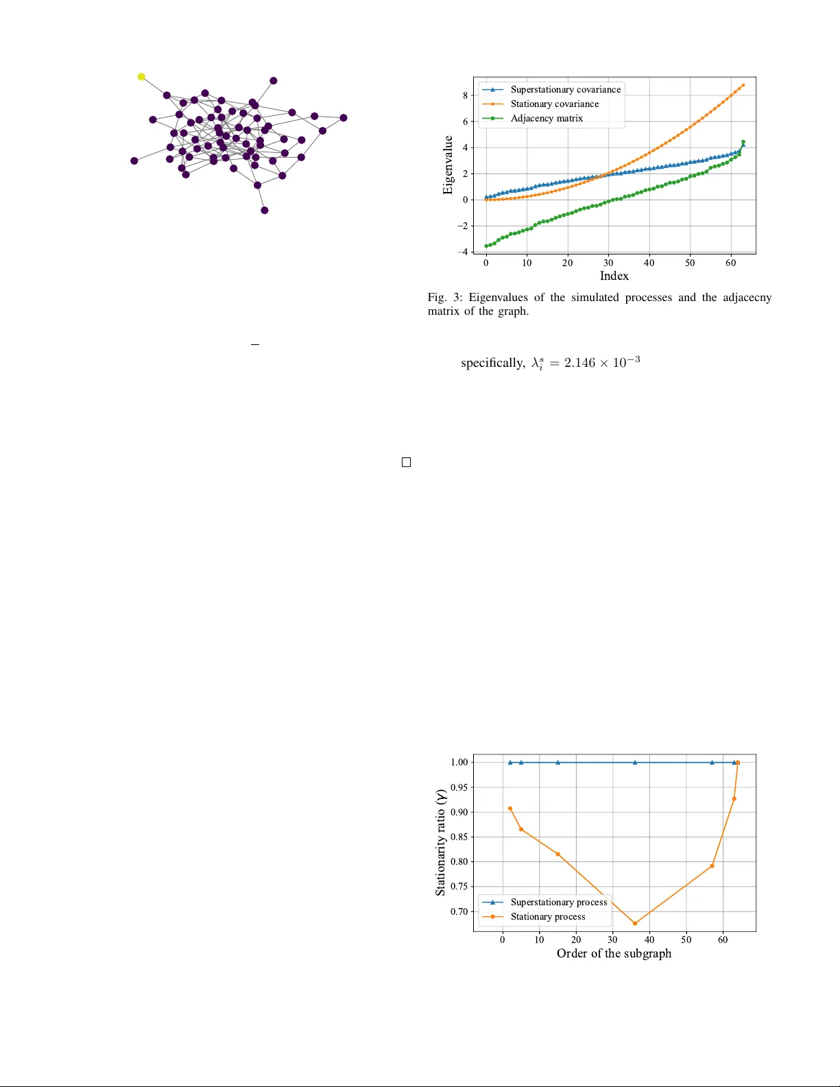
Piece wise Stationary Modeling of Random Processes Ov er Graphs W ith an Application to T raf fic Prediction Arman Hasanzadeh, Xi Liu, Nick Duf field and Krishna R. Narayanan Department of Electrical and Computer Engineering T exas A&M Uni versity College Station, T e xas 77840 Email: { armanihm, duffieldng , krn } @tamu.edu, xiliu.tamu@gmail.com Abstract —Stationarity is a key assumption in many statistical models f or random processes. With recent developments in the field of graph signal processing, the conventional notion of wide- sense stationarity has been extended to random processes defined on the v ertices of graphs. It has been sho wn that well-kno wn spec- tral graph kernel methods assume that the underlying random process over a graph is stationary . While many approaches hav e been proposed, both in machine learning and signal processing literature, to model stationary random processes over graphs, they are too restrictive to characterize real-w orld datasets as most of them are non-stationary pr ocesses. In this paper , to well- characterize a non-stationary process over graph, we propose a novel model and a computationally efficient algorithm that partitions a large graph into disjoint clusters such that the process is stationary on each of the clusters but independent across clusters. W e evaluate our model for traffic prediction on a large-scale dataset of fine-grained highway travel times in the Dallas–Fort W orth area. The accuracy of our method is very close to the state-of-the-art graph based deep learning methods while the computational complexity of our model is substantially smaller . Index T erms —Piecewise Stationary , Graph Clustering, Graph Signal Processing, T raffic Prediction I . I N T RO D U C T I O N Stationarity is a well-known h ypothesis in statistics and signal processing which assumes that the statistical charac- teristics of random process do not change with time [1]. Stationarity is an important underlying assumption for many of the common time series analysis methods [2]–[4]. With recent dev elopments in the field of graph signal processing [5]– [7], the concept of stationarity has been extended to random processes defined over vertices of graphs [8]–[11]. A random process over a graph is said to be graph wide-sense stationary (GWSS) if the cov ariance matrix of the process and the shift operator of the graph, which is a matrix representation of the graph (see Section II-B), hav e the same set of eigenv ectors. Incidentally , GWSS is the underlying assumption of spectral graph kernel methods which ha ve been widely used in machine learning literature to model random processes over graphs [12]–[16]. The core element in spectral kernel methods is the kernel matrix that measures similarity between random variables defined ov er vertices. This kernel matrix has the same set of eigenv ectors as the Laplacian matrix (or adjacency matrix) while its eigen v alues are chosen to be a function of eigen values of the Laplacian matrix (or adjacency matrix). Therefore, the kernel matrix and the shift operator of the graph share eigen vectors which is the exact definition of GWSS. While the stationarity assumption has certain theoretical and computational advantages, it is too restrictive for modeling real-world big datasets which are mostly non-stationary . In this paper , we propose a model that can deal with non-stationary cov ariance structure in random processes defined over graphs. The method we deploy is a nov el and computationally efficient graph clustering algorithm in which a large graph is partitioned into smaller disjoint clusters. The process defined over each cluster is stationary and assumed to be independent from other clusters. T o the best of our knowledge, our proposed clustering algorithm, stationary connected subgraph clustering (SCSC), is the first method to address this problem. Our model renders it possible to use highly-effecti ve prediction techniques based on stationary graph signal processing for each cluster [17]. An overvie w of our proposed clustering algorithm is shown in Fig. 1. Our work is analogous to piecewise stationary modeling of random processes in continuous space, which has been studied in the statistics literature. Howe ver , these methods cannot be extended to graphs due to discrete nature of graphs or the fact that the definition of GWSS is not inclusive (Section III-A). For instance, to model a non-stationary spatial process, Kim et al. [18] proposed a Bayesian hierarchical model for learning optimal V oronoi tessellation while Gramacy [19] pro- posed an iterativ e binary splitting of space (treed partitioning). Piecewise stationary modeling has also been explored in time series analysis which is mainly achiev ed by detecting change points [20], [21]. Recently , there has been an ef fort in graph signal processing literature to detect non-stationary vertices (change points) in a random process over graph [22], [23], howe ver , to achie ve that, authors introduce another definition for stationarity , called local stationarity , which is dif ferent from the widely-used definition of GWSS. W e ev aluate our proposed model for traffic prediction on a large-scale real-world traffic dataset consisting of 4764 ... ... ActiveComponent Extraction time StationaryConnected SubgraphClustering Dataset Active Components Stationary Clusters Fig. 1: An overvie w of our proposed stationary clustering algorithm. Given historical observation, i.e. time-series defined over nodes of a graph, first we extract active components. Ne xt, our proposed stationary connected subgraph clustering (SCSC) tries to merge adjacent active components to form stationary subgraphs. road se gments and time-series of a verage tra vel times on each segment at a two-minute granularity over January–March 2013. W e use simple piece wise linear prediction models within each cluster . The accuracy of our method is very close to the state-of-the-art deep learning method, i.e. only 0.41% difference in the mean absolute percentage error for 10 minute predictions, rising to 0.66% ov er 20 minutes. Howe ver , the learning time of our proposed method is substantially smaller, being roughly 3 hours on a personal computer while the deep learning method takes 22 hours on a server with 2 GPUs. Our contribution can be summarized as follows: • For the first time, we propose to model non-stationary random processes over graphs with piecewise stationary random processes. T o that end, we propose a nov el hierarchical clustering algorithm, i.e. stationary connected subgraph clustering, to extract stationary subgraphs in graph datasets. • W e theoretically prove that the definition of GWSS is not inclusive . Hence, unlik e many of the well-kno wn graph clustering algorithms, adding one vertex at each training step to clusters in an stationary clustering algorithm is bound to di ver ge. T o address this issue, we propose to use active components as input to stationary clustering algorithm instead of vertices. • W e ev aluate our proposed model for traffic prediction in road networks on a large-scale real-world traffic dataset. W e deploy an off-the-shelf piecewise linear prediction model for each subgraph, independently . Our method shows a very close performance to the state-of-the-art graph based deep learning methods while the computa- tional complexity of our model is substantially smaller . I I . B A C K G RO U N D A. Spectral Graph K ernels Kernel methods, such as Gaussian process and support vector machine, are a powerful and ef ficient class of algorithms that hav e been widely used in machine learning [12]. The core element in these methods is a positive semi-definite kernel function that measures the similarity between data points. For the data defined ov er vertices of a graph, spectral kernels are defined as a function of the Laplacian matrix of the graph [12]. More specifically , given a graph G with Laplacian matrix L , the kernel matrix K is defined as K = N X i =1 r ( λ i ) u i u i T . (1) Here, N is the number of vertices of the graph, λ i and u i are the i -th eigenv alue and eigen vector of L , respectiv ely , and the spectral transfer function r : R + → R + is a non-negativ e and decreasing function. Non-negati veness of r assures that K is positiv e semi-definite and its decreasing property guarantees that the kernel function penalizes functions that are not smooth ov er graph. Many of the common graph kernels can be deriv ed by choosing a parametric family for r . For example, r ( λ i ) = exp( − λ i / 2 σ 2 ) result in the well-known heat diffusion kernel. Although in the majority of the pre vious works, spectral graph kernels are derived from the Laplacian matrix, they can also be defined as a function of the adjacency matrix of the graph [16]. Adjacency based spectral kernels ha ve the same form as (1) except that the transfer function r is a non-negati ve and “increasing” function since eigenv ectors of adjacency with lar ge eigen v alues have smoother transitions over graph [24]. W e note that unlik e Laplacian matrix, eigenv alues of the adjacency matrix could be neg ativ e, therefore the domain of transfer function is R for adjacency based kernels. Spectral graph kernels have been widely used for semi- supervised learning [14], link prediction [25] and Gaussian process regression on graphs [13], [15]. In the next subsection, we sho w the connection between spectral graph k ernels and stationary stochastic processes ov er graphs. B. Stationary Graph Signal Pr ocessing Graph signal processing (GSP) is a generalization of clas- sical discrete signal processing (DSP) to signals defined over vertices of a graph (also known as graph signals ). Consider a graph G with N vertices and a graph signal defined ov er it denoted by a N -dimensional v ector x . The graph frequency domain is determined by selecting a shift operator S , i.e. a N × N matrix that respects the connectivity of vertices. Applying the shift operator to a graph signal, i.e. S x , is analogous to a circular shift in classical signal processing. The Laplacian matrix L and the adjacency matrix A are two examples of the shift operator . Let us denote the eigen values of S by { λ i } N i =1 and its eigen vectors by { u i } N i =1 . Also, assume that Λ = diag ( { λ i } N i =1 ) and U is a matrix whose columns are u i s. The graph Fourier transform (GFT) [5], [6] is defined as follows: Definition 1 (Graph Fourier transform [9]) . Gi ven graph G with shift operator S and a graph signal x defined over G , the Graph Fourier Transform (GFT) of x , denoted by ˆ x , is defined as ˆ x = U T x. (2) The in verse GFT of a vector in the graph frequency domain is giv en by x = U ˆ x. (3) It can be shown that when the Laplacian matrix is used as the shift operator , smoothness of eigenv ectors over the graph is proportional to their corresponding eigen value [5], and if the adjacency matrix is used as the shift operator , smoothness of eigen vectors over the graph is inv ersely proportional to their corresponding eigenv alues [24]. This ordering of eigen vectors provides the notion low-pass, band-pass and high-pass filters for graphs. More specifically , filtering graph signals is defined as shaping their spectrum with a function [26]–[28]. Definition 2 (Graph filters [9]) . Giv en a graph G with shift operator S , any function h : C → R defines a graph filter such that H = U h ( Λ ) U T . (4) The filtered version of a graph signal x defined ov er G is giv en by H x . An example of graph filter is the low pass diffusion filter . Assuming the Laplacian matrix is the shift operator , low pass diffusion filter h is defined as h ( λ i ) = exp( − λ i / 2 σ 2 ) . An important notion in classical DSP is stationarity of stochastic processes which is the underlying assumption for many of the well known time series analysis methods. Sta- tionarity of a time series means that the statistical properties of the process do not change over time. More specifically , a stochastic process is wide-sense stationary (WSS) in time if and only if its first and second moment are shift inv ariant in time. An equi valent definition of WSS process is that the eigen vectors of cov ariance matrix of a WSS process are the same as columns of discrete Fourier transform (DFT) matrix. By generalizing the definition of WSS to stochastic processes defined on graphs, graph wide-sense stationary (GWSS) [9], [11] is defined as follows: Definition 3 (Graph wide-sense stationary [9]) . A stochastic process x with cov ariance matrix C defined over vertices of a graph G with shift operator S is GWSS if and only if C is jointly diagonalizable with S , i.e. C and S hav e the same set of eigenv ectors. Equiv alently , the stochastic process x is GWSS if and only if it can be produced by filtering white noise using a graph filter . Spectral graph kernel methods, discussed in the previous subsection, model the co v ariance matrix of the process o ver graph with the kernel matrix. The kernel matrix have the same set of eigenv ectors as shift operator; hence, these methods assume that the random process they are operating on is GWSS. It is also worth noting that GWSS reduces to WSS in case of time series. Assume that time series is a graph signal defined o ver a directed ring graph with adjacency matrix as the shift operator . Multiplying the adjacency matrix with the vector of time series (applying shift operator) results in the circular shifted version of the time series by one. Therefore, definition of graph filters reduces to discrete filters in classical DSP . Moreover , the adjacenc y matrix of the directed ring graph is a circulant matrix whose eigen vectors are the same as the vectors that define the discrete Fourier transform. Hence, both definitions of GWSS reduce to classical definitions of WSS time series. While GWSS is defined for random processes over graphs, in many practical scenarios, the signal on each vertex is a time series itself (time-v arying graph signals). Stationarity can be further extended to time varying random processes ov er graphs. More specifically , a jointly wide-sense stationary (JWSS) process [8] is defined as follows: Definition 4 (Joint wide-sense stationarity [8]) . A time- varying random process X = [ x (1) . . . x ( T ) ] defined over graph G with shift operator S is JWSS if and only if the following conditions hold: • X is multiv ariate wide-sense stationary process in time; • cross cov ariance matrix of x ( t 1 ) and x ( t 2 ) for ev ery pair of t 1 and t 2 is jointly diagonalizable with S . An example of JWSS process is the joint causal model which is analogous to auto-regressi ve moving av erage (ARMA) models for multiv ariate WSS time-series. The joint causal model is defined as follows: x ( t ) = m X i =1 A i x ( t − i ) + q X j =0 B j E ( t − j ) , (5) where A i and B j are graph filters and E is the vector of zero mean white noise. This model can be used to predict time- varying graph signals. Giv en a time-varying graph signal, the parameters of the joint causal model, i.e. A i s and B j s, can be learned by minimizing the prediction error residuals which is the subject to the following nonlinear optimization problem: arg min { A i } m i =1 , { B j } q j =0 || x ( t ) − e x ( t ) ( { A i } m i =1 , { B j } q j =0 ) || , (6) where x is the true signal and e x is the output of the model. Generally , this is a computationally expensiv e optimization problem especially for large graphs. Loukas et al. [17] pro- posed an ef ficient way for finding the optimal filters. They prov ed that because graph frequency components of a JWSS process are uncorrelated, learning independent univ ariate pre- diction models along each graph frequency result in optimal filters for prediction. While both Gaussian process regression with spectral graph kernels and joint causal model showed promising results in predicting graph signals, the y suffer from tw o major issues. First, in a typical real-world traffic dataset with a very large graph, the process defined over the graph is often not GWSS, which in validates their underlying assumption. Secondly , the computational complexity of learning prediction model pa- rameters for a large graph is formidable. T o overcome afore- mentioned issues, we propose to split the whole graph into multiple connected disjoint subgraphs such that the process is stationary in each of them and then fitting prediction model to each indi vidual subgraph. In the next section, first we show that this clustering is a very comple x and difficult task and then we discuss our proposed computationally-efficient clustering method. I I I . M E T H O D O L O G Y Here, first in section III-A, we sho w that the definition of GWSS is not inclusive , i.e. if a random process defined over a graph is GWSS, the subprocess defined ov er a subgraph is not necessarily GWSS. This shows the difficulty of clustering a large graph into stationary subgraphs. Then, in section III-B we propose a heuristic graph clustering algorithm to find stationary subgraphs. In our analysis, without loss of generality , we assume that each of the time series defined on the vertices of the graph is WSS in time. Therefore we analyze random process over graphs which are not time-varying. Our analysis and proposed algorithm can simply be extended to time varying processes. Due to lack of space we ignore some of the proofs as they can be found in the references. A. The Challenge of Identifying Stationary Subgraphs Many graph clustering algorithms start with some initial clusters, like random clusters or ev ery vertex as a cluster , and then they try to mo ve vertices between clusters with the objectiv e of maximizing a cost function. W e first analyze how stationarity changes as a cluster grows or shrinks. This problem can be simplified to analyzing the stationarity of subprocesses defined ov er subgraphs. Assume a case where a process x with covariance matrix C defined ov er graph G with adjacency matrix A as shift operator is GWSS. The question we want to answer is that if we choose any subgraph of G , does the subprocess defined ov er it is GWSS too? The ideal case is that the subprocesses defined over all of the possible subgraphs of G are also GWSS. W e call such a process, superstationary . More specifically , a superstatioanry random process ov er graph is defined as follows: Definition 5 (Superstationary) . A random process x defined ov er graph G is graph wide-sense superstatioanary (or super- stationary for short) if and only if the following conditions hold: • x is graph wide-sense stationary over G ; • the subprocesses defined ov er all of the possible sub- graphs of G are also graph wide-sense stationary . T o analyze the necessary conditions for a random process ov er graph to be superstationary , first we deriv e an equiv alent definition for GWSS. Theorem 1. T wo squar e matrices are jointly diagonalizable if and only if the y commute [29]. Combining the above theorem with definition of GWSS (Definition 3), it is straightforward to show that a random process x with covariance matrix C defined over G is GWSS if and only if A C = C A . T o find a similar condition for superstationary random processes, first we revie w the definition of super commuting matrices from linear algebra literature. Definition 6 (Supercommuting matrices [30]) . T wo square matrices, B 1 and B 2 , supercommute if and only if the following conditions hold: • B 1 and B 2 commute; • each of the principal submatrices of B 1 and their corre- sponding submatrices of B 2 commute. Knowing the definitions of superstationary random process and supercommuting matrices, in the following theorem, we deriv e the necessary and suf ficient condition for a process to be superstationary . Theorem 2. A random process x with covariance matrix C defined over a graph with adjacency matrix A as the shift operator is super stationary if and only if A and C super commute. Pr oof. The adjacency matrix of a subgraph is a submatrix of A . Also, cov ariance matrix of a subprocess is a submatrix of C . By definition of superstationarity , subprocesses defined ov er all of the possible subgraphs of G are GWSS, hence all of the corresponding submatrices of A and C commute. While the theorem above shows the necessary and sufficient condition for superstationarity , directly checking it is compu- tationally expensiv e specially for large graphs. T o that end, we show that gi ven an adjacency matrix, only a class of cov ariance matrices are superstationary . T o continue our analysis, first we revie w the definition of irreducible matrix and then we study the matrices that supercommute with irreducible matrices. Definition 7 (Irreducible matrix [31]) . A matrix B is irre- ducible if and only if the directed graph whose weighted adjacency matrix is B , is strongly connected. Theorem 3. Any matrix that super commutes with irreducible squar e matrix B N × N is a linear combination of B and identity matrix I N [30]. Fig. 2: The simulated Erd ¨ os-Renyi graph. Next, we derive the sufficient and necessary condition for a process defined o ver a strongly connected graph to be superstationary . Theorem 4. A random pr ocess x with covariance matrix C defined over a str ongly connected graph of order N with adjacency matrix A as the shift operator is superstationary if and only if C is a linear combination of A and identity matrix I N . Pr oof. The adjacency matrix of a strongly connected graph is an irreducible matrix. Therefore, giv en Theorem 2, Definition 7 and Theorem 3, the proof is straightforward. Assuming that the desired graph G is strongly connected 1 , which is a realistic assumption in many of the real-world networks, unless C is a linear combination of A and identity matrix, there is at least a subgraph such that the subprocess defined over it is non-stationary . This is a major challenge for identifying stationary subgraphs. Suppose that we start with a subgraph containing only one vertex and add one verte x at a time until we cov er the whole graph and at each step we check whether the subprocess is stationary or not. W e know that at some step the subprocess is non-stationary . But being non-stationary at a step does not necessarily mean that the subprocess is non-stationary in the next steps as we know that the process in the last step is stationary . This means that moving one v ertex at a time between clusters is not optimal and the algorithm may not con verge at all. Next, we show the diffe rence of a stationary process and a superstationary process with an example. W e generate a random Erd ¨ os-Renyi graph with 64 nodes with edge probability of 0.06 (shown in Fig. 2). W e form two cov ariance matrices, a stationary and a superstationary , as follows: 1) W e eigendecompose the adjacency matrix and assume that the covariance matrices of stationary and supersta- tionary processes ha ve the same set of eigen vectors as adjacency matrix. Let us denote the eigenv alues of the adjacency matrix by { λ i } N i =1 . 2) W e choose the eigen v alues of the stationary cov ariance matrix to be quadratic function (shown in Fig. 3). More 1 Undirected graphs are strongly connected as long as they are connected. 0 10 20 30 40 50 60 Index 4 2 0 2 4 6 8 Eigenvalue Superstationary covariance Stationary covariance Adjacency matrix Fig. 3: Eigen values of the simulated processes and the adjacecny matrix of the graph. specifically , λ s i = 2 . 146 × 10 − 3 i 2 + 1 . 073 × 10 − 5 for i ∈ { 1 , . . . , 64 } . 3) W e choose the the eigenv alues of the superstationary cov ariance matrix to be linear function of eigenv alues of the adjacency matrix (shown in Fig. 3). More specif- ically , λ ss i = 0 . 5 λ i + 2 for i ∈ { 1 , . . . , 64 } . W e start with a subgraph consisting of a randomly chosen node (the yellow node in Fig. 2) and its immediate neighbors and compute the stationarity ratio of the processes ov er this subgraph. W e keep increasing the size of the subgraph by adding one-hop neighbors of the nodes in the subgraph (at the current step) to it and compute the stationarity ratio at each step. The results are shown in Fig. 4. As we expected, the superstationary process is completely stationary on all of subgraphs while the stationary ratio of the stationary process could decrease to less than 0.7 for some of the subgraphs. This, indeed, shows the challenge of stationary graph clustering and prov es that moving one vertex at a time between clusters could cause the algorithm to div erge from the optimal solution. In the next subsection we propose a heuristic approach to overcome this problem. 0 10 20 30 40 50 60 Order of the subgraph 0.70 0.75 0.80 0.85 0.90 0.95 1.00 S t a t i o n a r i t y r a t i o ( ) Superstationary process Stationary process Fig. 4: Stationary ratio of the simulated processes over subgraphs. 1 3 2 5 8 6 7 4 1 3 2 5 8 6 7 4 1 3 2 5 8 6 7 4 1 3 2 5 8 6 7 4 T ime Fig. 5: V isualization of an active component of a graph. At the fist snapshot, node 4 becomes active and as time goes by the activity spreads in the network. The red nodes at each snapshot represents activ e nodes. The subgraph containing nodes 1, 3, 4, 5, 6 and 7 is an acti ve component of the network. B. Stationary Connected Subgraph Clustering W e are interested in modeling a non-stationary random process over a graph using a piecewise stationary process over the same graph. Therefore, the stationary graph clustering problem is defined as follows: Problem 1. Giv en a graph G and a non-stationary stochastic process x defined over G , partition the graph into k disjoint connected subgraphs {G 1 , G 2 , . . . , G k } such that each of the subprocesses { x 1 , x 2 , . . . , x k } defined over subgraphs are GWSS. W e propose a heuristic algorithm, stationary connected subgraph clustering (SCSC), to solve the problem abov e. T o the best of our knowledge, we address this problem for the first time. As we discussed in the previous subsection, adding one verte x at a time to identify stationary subgraphs is problematic. Therefore, we propose a clustering algorithm whose inputs are active components rather than vertices. Active components (A Cs) are spatial localization of activity patterns made by the process over the graph (see Fig. 5). Spatial spreading of congestion in transportation networks and spreading pattern of rumor in social networks are two examples of activ e components. First, we clarify the mathematical definition of a verte x being active . If magnitude of the signal defined over a verte x exceeds a threshold, i.e. x [ i ] ≥ α , we say that the vertex is active. For example, if the tra vel time of a road exceeds a threshold it means that it is congested or activ e. Knowing the mathematical definition of activ e vertex, activ e component is defined as follows: Definition 8 (Activ e component) . W e say that the vertex i and verte x j are in the same activ e component if and only if at some time t both of the following conditions hold: • ( i, j ) or ( j, i ) is an edge of the graph; • vertex i is active at time t and vertex j is activ e at time t or t − 1 or vice versa. A Cs can be viewed as subgraphs on which a diffusion process takes place. W e already know that diffusion processes are stationary processes. Therefore, we expect that the subpro- cesses defined over A Cs to be stationary . T o obtain A Cs from Algorithm 1 Activ e Components Extraction 1: Input: G , α, Y ∈ R N × T 2: Notations: 3: G = network graph 4: α = threshold on signal determining activ e vertices 5: Y = historical observation matrix 6: Initialize: 7: A C ← {} , A C t ← {} , A C t − 1 ← {} 8: for i = 1 : T do 9: R ← argwhere ( Y (: , i ) < α ) 10: G sub ← remove R and connected edges from G 11: A C t ← connected components of G sub 12: for j = 1 : len ( A C t − 1 ) do 13: indicator ← False 14: for k = 1 : len ( AC t ) do 15: A C t ( k ) ← one hop expansion of A C t ( k ) 16: if (A C t ( k ) ∩ A C t − 1 ( j )) 6 = ∅ then 17: A C t ( k ) ← (A C t ( k ) ∪ A C t − 1 ( j )) 18: indicator ← True 19: if indicator == False then 20: append A C t − 1 ( j ) to A C 21: retur n A C historical observ ations, we propose the activ e components extraction iterativ e algorithm. The overvie w of Algorithm 1 is that at each time step, first we create the active graph by removing the inacti ve nodes and all the edges connected to these nodes from the whole network graph. Then we go through time and if activity patterns at time t − 1 are propagating to time t , the activ e components are merged into one. In fact, the algorithm finds weakly connected components of the strong product of spatial graph and time- series graph when spatio-temporal nodes with signal amplitude less than α and all of connected edges to them are remov ed. Before we describe the second part of the algorithm in which the adjacent ACs are merged and form clusters, we revie w the measure of stationarity defined in [8]. First, we form the following matrix P = U T C U , (7) where U is the matrix of eigen vectors of the shift operator and Algorithm 2 Stationary Connected Subgraph Clustering 1: Input: G , γ th , C , AC , θ , D 2: Notations: 3: G = network graph 4: γ th = threshold on stationarity ratio 5: C = cov ariance matrix 6: A C = set of activ e components 7: θ = number of clusters 8: D = matrix of distances between activ e components 9: Initialize: 10: CLS ← A C , NL ← {} , n ← | A C | 11: while n > θ do 12: d min ← min ( D ) 13: [ i, j ] ← arg min ( D ) 14: if d min < 2 and [ i, j ] * NL then 15: CT ← ( A C ( i ) ∪ A C ( j )) 16: G sub ← induced subgraph of G for nodes in CT 17: C sub ← C [ CT , CT ] 18: γ ← compute stationarity ratio using C sub & G sub 19: if γ ≥ γ th then 20: remov e AC ( i ) and A C ( j ) from CLS 21: insert CT to CLS 22: update D in single linkage manner 23: n ← n − 1 24: else append [ i, j ] to NL 25: if | NL | == | CLS | then 26: break 27: retur n CLS C is the cov ariance matrix of the random process. Stationarity ratio, γ , of a random process ov er graph is defined as follows: γ = || diag ( P ) || 2 || P || F , (8) where || . || F represents the Frobenius norm and diag(.) denotes the vector of diagonal elements of the matrix. In fact, γ is a measure of diagonality of matrix P . If a process is GWSS then eigen vectors of cov ariance matrix and shift operator of the graph are the same hence P is diagonal and γ equals to one. Diagonal elements of P form the power spectral density of the GWSS process. Another definition that we need to move forward to the next step is the distance between two A Cs. The distance between two ACs is the minimum of the shortest path distances between all pairs of nodes ( v 1 , v 2 ) where v 1 ∈ A C 1 and v 2 ∈ A C 2 . W e note that two A Cs could have a common node, hence the distance between two A Cs could be zero. Knowing all necessary definitions, the psudocode for SCSC algorithm is described in Algorithm 2. The intuition behind SCSC is that it is most likely that adjacent ACs belong to the same diffusion process. SCSC merges adjacent A Cs if after mer ger the stationarity ratio is larger than some threshold. This definition makes sense since it is repeatedly observed that activity on one vertex easily causes or serves as a result of acti vity in the adjacent v ertex with some time difference. Therefore, we expect that the process defined ov er the output clusters of SCSC to be stationary . SCSC is a hierarchical clustering algorithm with some extra conditions. The overload caused by these conditions are small compared the complexity of hierarchical clustering. The conditions only needs eigendecomposition of small matrices (usually less than 50 × 50 ) which is negligible. While SCSC algorithm, as defined in Algorithm 2, extracts subgraphs that are GWSS, with a simple modification to the algorithm, we can identify subgraphs that are JWSS. Assuming that a time v arying random process X is WSS in time, the necessary condition for X to be JWSS is that all of the lagged auto-cov ariance matrices are jointly diagonalizable with S . Hence, lines 17 to 19 in Algortihm 2 (the merger condition of clusters in SCSC) are replaced by the following lines:           for l = 0 : q do C ( l ) sub ← C ( l ) [ CT , CT ] γ l ← compute stationarity ratio using C ( l ) sub & G sub if γ l ≥ γ th for l = 0 : q then where C ( l ) is the cross cov ariane between x ( t ) and x ( t − l ) and q is a hyper-parameter denoting maximum lag. Note that both C ( l ) and q are inputs of the algorithm. C. Application to T raffic Pr ediction T o examine our model, we use our proposed approach for trav el time prediction in road networks. First, we use line graph of transportation network to map roads into vertices of a directed graph. Then, we use trav el time index (TTI) [32] to extract activ e components from historical data. TTI of a road segment is defined as its current travel time divided by the free flow travel time of the road segment or, equiv alently , the free flow speed divided by the current average speed. TTI can be interpreted as a measure of sev erity of congestion in a road segment. W e also propose using the joint causal model (5) for each cluster separately . T o capture the dynamic and non-linear behavior of traffic, we propose using a piecewise linear model as prediction model for time series along each graph frequency . More specifically , threshold auto-regressiv e (T AR) [33], [34] models are piece-wise linear extension of linear AR models. The T AR model assumes that a time-series can hav e se veral regimes and its behavior is different in each regime. The regime change could be triggered either by past values of the time-series itself (self exciting T AR [35]) or some exogenous variable. This model is a good candidate to model the traf fic behavior; once a congestion happens, the dynamics of time- series changes. A T AR model with l regimes is defined as follows: y t =            P m 1 i =1 a (1) i y ( t − i ) + b (1)  t , β 0 < z t < β 1 P m 2 i =1 a (2) i y ( t − i ) + b (2)  t , β 1 < z t < β 2 . . . P m l i =1 a ( l ) i y ( t − i ) + b ( l )  t , β l − 1 < z t < β l Fig. 6: The map of the road network in Dallas. where z is the exogenous variable. A natural choice of exogenous variable for traffic is TTI, because it shows sev erity of congestion. I V . N U M E R I C A L R E S U LT S A N D D I S C U S S I O N A. Dataset The traf fic data used in this study originated from the Dallas-Forth W orth area, with a graph comprising 4764 road segments in the highway network. The data represented time- series of average trav el times as well as average speed on each segment at a two-minute granularity over January–March 2013. The data was used under licence from commercial data provider , which produces this data applying proprietary methods to a number of primary sources including location data supplied by mobile device applications. Fig. 6 shows the map of the road network. Missing values form dataset were imputed by moving average filters. In all experiments, we used 70% of data for training, 10% for validation and 20% for testing. B. Experimental Setup 1) Our Pr oposed Method: After removing daily seasonality from time series, difference transformation was used to make the time series along each vertex WSS. Augmented Dicky- Fuller test was used to check for stationarity in time. W e used 1.7 as threshold ( α = 1 . 7 ) for TTI to detect congestion in a road. 117621 active components were extracted from the training data using Algorithm 1. W e eliminated A Cs with less than 5 vertices which reduced the number of A Cs to 52494. In our clustering algorithm, we used combinatorial Lapla- cian matrix of directed graphs [36], which is defined as follo ws L = 1 2 ( D out + D in − A − A T ) , as the shift operator . In the equation above, D out and D in represent the out-degree and in-degree matrices, respecti vely . The in-degree (out-degree) matrix is a diagonal matrix whose i -th diagonal element is equal to the sum of the weights of all the edges entering (leaving) vertex i . Probability density Stationarity ratio Fig. 7: The histogram of stationarity ratio of subprocesses defined ov er active components. W e initiated the SCSC algorithm (Algorithm 2) by setting minimum stationarity ratio to 0.9 and number of clusters to 150. The number of vertices in clusters are between 24 to 61. Prediction models were learned for each cluster independently in the graph frequency domain. T AR models consist of three different regimes. The exogenous threshold variable for our proposed prediction models, joint causal model with T AR (JCM-T AR), is the sum of TTI values of all nodes in a cluster at each time step. This value shows how congested the whole cluster is. W e implemented our clustering algorithm in Python and used tsDyn package [37] in R to learn the parameters of (threshold) auto-regressi ve models. 2) Baselines: T o establish accuracy benchmarks, we con- sider four other prediction models. The first scheme is to build independent auto-regressi ve integrated moving average (ARIMA) [38] models for time series associated with each road. After removing daily seasonality form data, ARIMA models with fiv e moving average lags and one auto-regressi ve lag were learned. This naiv e scheme ignores the spatial corre- lation of adjacent roads. The second benchmark scheme is a joint causal model with non-adaptiv e AR models (JCM- AR) in graph frequency domain of each cluster . W e used the same clusters as our proposed method discussed in pre vious subsection. The third scheme is the diffusion con volutional recurrent neural network (DCRNN) [39]. This deep learning method uses long short-term memory (LSTM) cells on top of diffusion con volutional neural network for traffic prediction. The archi- tecture of DCRNN includes 2 hidden RNN layers, each layer includes 32 hidden units. Spatial dependencies are captured by dual random walk filters with 2-hop localization. The last baseline is the spatio-temporal graph conv olutional neural network (STGCN) [40]. This method uses graph con volutional layers to extract spatial features and deploys one dimensional con volutional layers to model temporal behavior of the traffic. W e used two graph con volutional layers with 32 Chebyshe v T ABLE I: Traf fic prediction performance of our proposed method and baselines. T Metric ARIMA DCRNN STGCN JCM-AR JCM-T AR 10 min MAE 2.7601 1.1764 1.0437 2.0520 1.2732 RMSE 5.3204 2.7553 2.6370 4.8620 2.9993 MAPE 5.10% 2.68% 2.44% 4.28% 2.85% 14 min MAE 3.3427 1.3837 1.1586 3.1187 1.7415 RMSE 6.5432 3.1186 2.8682 5.3481 3.5231 MAPE 8.32% 3.22% 3.11% 7.84% 3.51% 20 min MAE 4.9971 1.5948 1.3911 4.3873 1.9926 RMSE 10.8734 3.5287 3.3406 10.0381 4.0154 MAPE 13.65% 3.83% 3.67% 12.75% 4.33% filters. W e also used two temporal gated conv olution layers with 64 filters each. W e used the Python implementations of DCRNN and STGCN provided by the authors. C. Discussion T o check our hypothesis that active components are station- ary , we look at the probability density of stationarity ratios of data defined over of active components (showed in Fig. 7). W e note that most of the A Cs hav e stationarity ratio of more than 0.8 which approv es our hypothesis. W e also compare our proposed SCSC with spectral cluster- ing [41] and normalized cut clustering [42] algorithms. The av erage stationarity ratio of clusters for spectral clustering and normalized cut clustering are 0.4719 and 0.3846, respectively , while our SCSC algorithm produces clusters with stationarity ratio of more than 0.9. SCSC shows superior performance in finding stationary clusters as other clustering algorithms hav e different objectiv es. T able I sho ws the prediction accuracy of the proposed method and baselines for 10 minutes, 14 minutes and 20 minutes ahead traffic forecasting. The metrics used to ev aluate the accuracy are mean absolute error (MAE), mean abso- lute percentage error (MAPE) and root mean squared error (RMSE); see [39]. ARIMA sho ws the worst accuracy because it does not capture spatial correlation between neighboring roads and it cannot capture dynamic temporal behavior of traffic using a linear model. JCM-AR improves the the performance of ARIMA because it uses spatial correlation implicitly . The difference between these two models shows the importance of spatial dependencies. The improvement is more substantial for long term predictions. JCM-T AR model with three regimes shows the second best performance. This shows that temporal dynamic behavior of traffic is changing once a congestion happens in the network because a congestion can change the statistics of the process drastically . W e note that the perfor - mance of JCM-T AR is v ery close to DCRNN especially for short term traffic prediction. Howe ver , the small enhancement of DCRNN comes with a huge increase in model complexity and scalability . T o learn the parameters of DCRNN and STGCN, we used a server with 2 GeForce GTX 1080 Ti GPUs which took more than 22 and 11 hours to con ver ge, respecti vely . Doubling the number of hidden units in the RNN layers of DCRNN to 64 units, the server ran out of memory . Ho wev er, it took less than 3 hours for our method to con ver ge using a computer with 2.8GHz Intel Corei7 CPU and 16GB of RAM to simulate our method. The activ e components extraction took less than an hour and the SCSC algorithm conv erged in less than 2 hours. Estimation of our proposed prediction models are very fast because we used univ ariate piecewise linear models both in time and space which can be implemented completely in parallel. Another advantage of our method is the complexity of parameter tuning. While the parameters in our model are inter- pretiv e and most of them do not need any tuning, deep method could be very sensitive to network architecture. Extensiv e search ov er different parameters is the common way in deep learning to find the best architecture. It took us days to tune the parameters of DCRNN. Deep learning models can predict the traffic with very high accuracy [39], [40], [43]–[46] but most of them ignore complexity and scalability of the model to real world big datasets. Howe ver , a carefully designed prediction model, for short term traffic prediction, can perform as well as deep learning with less complexity and better scalability . V . C O N C L U S I O N In this work, we introduced a ne w method for modeling non-stationary random processes over graphs. W e proposed a nov el graph clustering algorithm, called SCSC, in which a large graph is partitioned into smaller disjoint clusters such that the process defined over each cluster is assumed to be stationary and independent from other clusters. Independent prediction models for each cluster can be deployed to predict the process. Numerical results showed that combining our piecewise stationary model with a simple piecewise linear prediction model shows comparable accuracy to graph based deep learning methods for traffic prediction task. More specif- ically , the accuracy of our method is only 0.41 lower in mean absolute percentage error to the state-of-the-art graph based deep learning method, while the computational complexity of our model is substantially smaller , with computation times of 3 hours on a commodity laptop, compared with 22 hours on a 2-GPU array for deep learning methods. V I . A C K N O W L E D G E M E N T S This material is based upon work supported by the National Science Foundation under Grant ENG-1839816. R E F E R E N C E S [1] A. Papoulis, Pr obability , random variables, and stochastic processes , ser . McGraw-Hill series in systems science. McGraw-Hill, 1965. [2] D. A. Dickey and W . A. Fuller , “Distrib ution of the estimators for autoregressi ve time series with a unit root, ” Journal of the American Statistical Association , vol. 74, no. 366a, pp. 427–431, 1979. [3] P . J. Brockwell and R. A. Davis, Stationary Pr ocesses . Cham: Springer International Publishing, 2016, pp. 39–71. [4] J. D. Cryer and N. Kellet, Models F or Stationary T ime Series . New Y ork, NY : Springer New Y ork, 2008, pp. 55–85. [5] D. I. Shuman, S. K. Narang, P . Frossard, A. Ortega, and P . V an- derghe ynst, “The emerging field of signal processing on graphs: ex- tending high-dimensional data analysis to networks and other irregular domains, ” IEEE Signal Processing Magazine , vol. 30, no. 3, pp. 83–98, 2013. [6] A. Sandryhaila and J. M. F . Moura, “Big data analysis with signal processing on graphs: Representation and processing of massi ve data sets with irregular structure, ” IEEE Signal Pr ocessing Magazine , vol. 31, no. 5, pp. 80–90, Sept 2014. [7] A. Ortega, P . Frossard, J. Kov a ˇ cevi ´ c, J. M. Moura, and P . V andergheynst, “Graph signal processing: Overview , challenges, and applications, ” Pr o- ceedings of the IEEE , vol. 106, no. 5, pp. 808–828, 2018. [8] A. Loukas and N. Perraudin, “Stationary time-vertex signal processing, ” arXiv preprint arXiv:1611.00255 , 2016. [9] A. G. Marques, S. Segarra, G. Leus, and A. Ribeiro, “Stationary graph processes and spectral estimation, ” vol. 65, no. 22, Nov 2017, pp. 5911– 5926. [10] N. Perraudin, A. Loukas, F . Grassi, and P . V anderghe ynst, “T owards stationary time-vertex signal processing, ” in 2017 IEEE International Confer ence on Acoustics, Speech and Signal Pr ocessing (ICASSP) , March 2017, pp. 3914–3918. [11] N. Perraudin and P . V anderghe ynst, “Stationary signal processing on graphs, ” IEEE T ransactions on Signal Processing , vol. 65, no. 13, pp. 3462–3477, July 2017. [12] A. J. Smola and R. Kondor , “Kernels and regularization on graphs, ” in Learning theory and kernel machines . Springer , 2003, pp. 144–158. [13] P . Sollich, M. Urry , and C. Coti, “K ernels and learning curv es for gaussian process regression on random graphs, ” in Advances in Neural Information Processing Systems 22 , Y . Bengio, D. Schuurmans, J. D. Lafferty , C. K. I. Williams, and A. Culotta, Eds. Curran Associates, Inc., 2009, pp. 1723–1731. [14] J. Zhu, J. Kandola, Z. Ghahramani, and J. D. Lafferty , “Nonparametric transforms of graph kernels for semi-supervised learning, ” in Advances in neural information pr ocessing systems , 2005, pp. 1641–1648. [15] M. J. Urry and P . Sollich, “Random walk kernels and learning curves for gaussian process regression on random graphs, ” The Journal of Machine Learning Researc h , vol. 14, no. 1, pp. 1801–1835, 2013. [16] K. A vrachenkov , P . Chebotare v , and D. Rubanov , “Similarities on graphs: Kernels versus proximity measures, ” European Journal of Combina- torics , 2018. [17] A. Loukas, E. Isufi, and N. Perraudin, “Predicting the e volution of stationary graph signals, ” in 2017 51st Asilomar Confer ence on Signals, Systems, and Computers , Oct 2017, pp. 60–64. [18] H.-M. Kim, B. K. Mallick, and C. C. Holmes, “ Analyzing nonstationary spatial data using piecewise gaussian processes, ” Journal of the Ameri- can Statistical Association , vol. 100, no. 470, pp. 653–668, 2005. [19] R. B. Gramacy , “Bayesian treed gaussian process models, ” Ph.D. dis- sertation, University of California, Santa Cruz, 2005. [20] U. Appel and A. V . Brandt, “ Adaptiv e sequential segmentation of piecewise stationary time series, ” Information sciences , vol. 29, no. 1, pp. 27–56, 1983. [21] M. Last and R. Shumway , “Detecting abrupt changes in a piecewise locally stationary time series, ” Journal of multivariate analysis , vol. 99, no. 2, pp. 191–214, 2008. [22] B. Girault, S. S. Narayanan, and A. Ortega, “Local stationarity of graph signals: insights and experiments, ” in W avelets and Sparsity XVII , vol. 10394. International Society for Optics and Photonics, 2017, p. 103941P . [23] A. Serrano, B. Girault, and A. Orteg a, “Graph variogram: A novel tool to measure spatial stationarity , ” in 2018 IEEE Global Conference on Signal and Information Processing (GlobalSIP) . IEEE, 2018, pp. 753–757. [24] A. Sandryhaila and J. M. F . Moura, “Discrete signal processing on graphs: Frequency analysis, ” IEEE Tr ansactions on Signal Processing , vol. 62, no. 12, pp. 3042–3054, June 2014. [25] J. Kunegis and A. Lommatzsch, “Learning spectral graph transforma- tions for link prediction, ” in Pr oceedings of the 26th Annual Interna- tional Conference on Machine Learning . A CM, 2009, pp. 561–568. [26] N. Tremblay , P . Gonc ¸ alves, and P . Borgnat, “Design of graph filters and filterbanks, ” in Cooperative and Graph Signal Processing . Elsevier , 2018, pp. 299–324. [27] A. Sandryhaila and J. M. Moura, “Discrete signal processing on graphs: Graph filters, ” in 2013 IEEE International Conference on Acoustics, Speech and Signal Pr ocessing . IEEE, 2013, pp. 6163–6166. [28] J. Liu, E. Isufi, and G. Leus, “Filter design for autoregressi ve moving av erage graph filters, ” IEEE T ransactions on Signal and Information Pr ocessing over Networks , vol. 5, no. 1, pp. 47–60, 2018. [29] R. Horn, R. Horn, and C. Johnson, Matrix Analysis . Cambridge Univ ersity Press, 1990. [30] C. C. Haulk, J. Drew , C. R. Johnson, and J. H. T art, “Characterization of supercommuting matrices, ” Linear and Multilinear Algebra , vol. 43, no. 1-3, pp. 35–51, 1997. [31] A. Jeffrey and D. Zwillinger, “13 - matrices and related results, ” in T able of Integr als, Series, and Pr oducts (Sixth Edition) , sixth edition ed. San Diego: Academic Press, 2000, pp. 1059 – 1064. [32] W . Pu, “ Analytic relationships between travel time reliability measures, ” T ransportation Researc h Recor d , vol. 2254, no. 1, pp. 122–130, 2011. [33] K.-S. Chan et al. , “T esting for threshold autoregression, ” The Annals of Statistics , vol. 18, no. 4, pp. 1886–1894, 1990. [34] K. S. Chan and H. T ong, “On estimating thresholds in autoregressive models, ” Journal of time series analysis , vol. 7, no. 3, pp. 179–190, 1986. [35] J. Petruccelli and N. Davies, “ A portmanteau test for self-exciting threshold autoregressiv e-type nonlinearity in time series, ” Biometrika , vol. 73, no. 3, pp. 687–694, 1986. [36] F . Chung, “Laplacians and the Cheeger inequality for directed graphs, ” Annals of Combinatorics , vol. 9, no. 1, pp. 1–19, 2005. [37] A. F . Di Narzo, J. L. Aznarte, and M. Stigler , dplyr: Nonlinear Time Series Models with Re gime Switching , 2019, r package version 0.9-48.1. [Online]. A vailable: https://CRAN.R- project.org/package=tsdyn [38] R. McCleary , R. A. Hay , E. E. Meidinger, and D. McDowall, Applied time series analysis for the social sciences . Sage Publications Be verly Hills, CA, 1980. [39] Y . Li, R. Y u, C. Shahabi, and Y . Liu, “Dif fusion conv olutional recurrent neural network: Data-driven traffic forecasting, ” in International Con- fer ence on Learning Representations , 2018. [40] B. Y u, H. Y in, and Z. Zhu, “Spatio-temporal graph conv olutional net- works: A deep learning framework for traffic forecasting, ” in Proceed- ings of the 27th International Joint Conference on Artificial Intelligence , ser . IJCAI’18. AAAI Press, 2018, pp. 3634–3640. [41] A. Y . Ng, M. I. Jordan, and Y . W eiss, “On spectral clustering: Anal- ysis and an algorithm, ” in Advances in neural information processing systems , 2002, pp. 849–856. [42] I. S. Dhillon, Y . Guan, and B. Kulis, “K ernel k-means: spectral clustering and normalized cuts, ” in Pr oceedings of the tenth ACM SIGKDD international conference on Knowledge discovery and data mining . A CM, 2004, pp. 551–556. [43] Y . Lv , Y . Duan, W . Kang, Z. Li, and F . W ang, “Traf fic flow prediction with big data: A deep learning approach, ” IEEE T ransactions on Intelligent T ransportation Systems , vol. 16, no. 2, pp. 865–873, April 2015. [44] R. Y u, Y . Li, C. Shahabi, U. Demiryurek, and Y . Liu, “Deep learning: A generic approach for extreme condition traffic forecasting, ” in Pr o- ceedings of the 2017 SIAM International Conference on Data Mining . SIAM, 2017, pp. 777–785. [45] Y . W u and H. T an, “Short-term traf fic flo w forecasting with spatial- temporal correlation in a hybrid deep learning framework, ” arXiv pr eprint arXiv:1612.01022 , 2016. [46] X. Ma, Z. Dai, Z. He, J. Ma, Y . W ang, and Y . W ang, “Learning traffic as images: a deep con volutional neural network for large-scale transportation network speed prediction, ” Sensors , vol. 17, no. 4, p. 818, 2017.