Gradient-Based STL Control with Application to Nonholonomic Systems

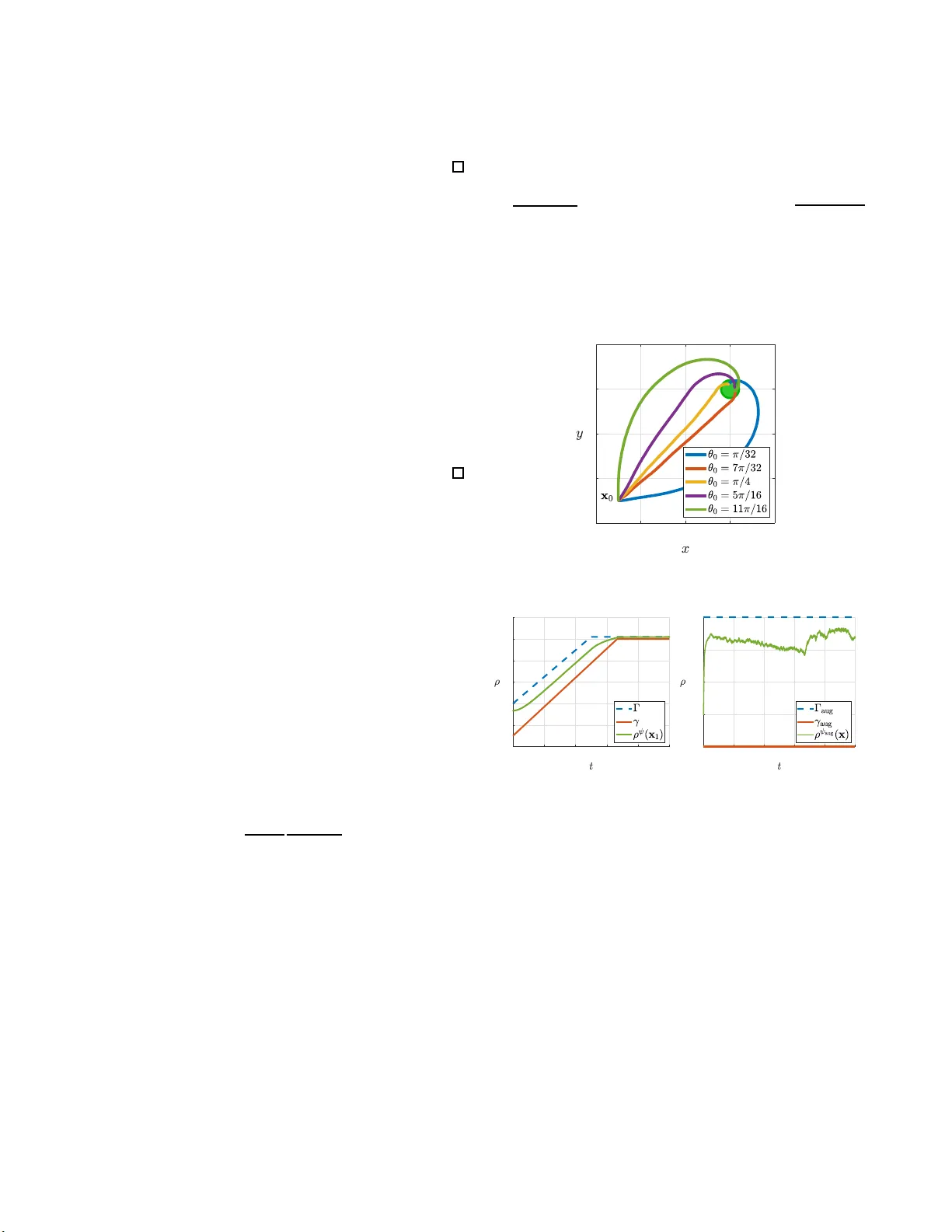
Gradient-Based STL Control with A pplication to Nonholonomic Systems Peter V arnai and Dimos V . Dimarogonas 1 Abstract — In this paper , we study th e control of dynamical systems under temporal logic task specifi cations using gradient- based meth od s relying on quantitative measures that express the extent to which the tasks are satisfied . A class of controllers capable of prov idin g satisfaction guarantees for simple systems and specifications is i ntroduced and then extended f or the case of u nicycle-like dynamics. The possibility of combining such controllers in order to tackle more complex task specifications while reta ini ng their computational efficiency is examined, and the practicalities re lated to an effective combination are demo n- strated th rough a simulation study . The introduced framewor k fo r controller design lays ground for future work in the direction of effective ly combin ing such elementary controllers fo r the purpose of aidin g exploration in l earning algorithms. I . I N T R O D U C T I O N In th is work , we in vestigate control strategies f o r ro botic systems subject to so-called temporal lo gic (TL) task spec- ifications. T empo ral logics ha ve many forms an d allow an expression of rich and com p lex tasks throu gh a combination of Boole a n and tempo ral op e r ators. Designing co ntrol strate- gies wh ich guar antee that the system exhibits the d esired behavior ha s ga ined co nsiderable in terest and is generally perfor med by abstracting th e s ystem space and ap plying solution tech niques over such a d iscretized d omain thr ough high-level planning algorith ms [1 ]. Signal tem p oral logic (STL) is a specific type of TL which enables expressing tasks directly related to the system, with- out ab stra c tion. The atomic pred icates serving as a ba sis for these expressions are defined over function s of continu ous- time system signals [2]. STL allo ws placing tempora l speci- fications on th e ev olution of these atomic predicates. This is useful in scenarios where explicit timing is important, such as having a rob ot visit a chargin g station within a fixed time sp an after its battery lo w ind icator goes of f. Pre vious works a im to provide con trollers fo r so lving STL tasks using methods related to, e.g., m o del predictive c o ntrol (MPC) [3] or prescribe d per f ormance control (PPC) [4]. Reinf o rcement learning methods hav e also gaine d attention recently [5] due to their success in oth er T L languag es [6 ]. Learning me thods offer the po ssibility of dealin g with unknown system dyn amics as well as to potentially reuse gathered experience to tackle new task s [7 ]. Howev er, they rely on a mu ltitude of simulations and experiments, which This work was partially supported by the W alle nberg AI, Auton omous Systems and Software Program (W ASP) funded by the Knut and Alice W al lenberg Founda tion, the Swedish Research Council (VR), the SSF COIN project , and the EU H2020 Co4Robots projec t. 1 Both aut hors are with the Di vision of Decisio n and Control Systems, School of Electric al Engineering and Computer Science, KTH Royal Insti- tute of T echnology , 114 28 Stockho lm, Sweden. varn ai@kth.se (P . V arnai), dimos@kth.se (D. V . Dimarogonas) makes computationa l an d samp le ef ficiency crucial fo r their usability in practice, such as in the case o f th e policy improvement algorithm [8]. Our work a ims towards ad- dressing this issue by presenting a framework for designin g inexpensive, gra dient-based con trollers wh ose pu rpose is to guide exploration in such learning methods. Such gu id ance has been shown to yield significant improvements in the perfor mance of po licy impr ovement [9], [10]. The contro llers sacrifice task satisfaction guarantees in exchange for co mpu- tational efficiency as they are co mputed from an ensemble of elementary contro llers related to simple su b tasks. The m a in con tr ibutions o f the work p r esented in this paper are outlined as f ollows. First, a class of contro ller s with task satisfaction g uarantees for simple task s and dy n amical sy s- tems is intro duced. These con trollers stem from prescribing the ev olutio n o f a task satisfaction metric in time, based on ideas f rom PPC [11] as in [4]. Th e introd u ced framew or k is then u sed to extend the range of system dyn amics which can be ha n dled to un icycle-like mod els. Finally , w e lay out initial though ts regardin g h ow to combine the derived controllers, e.g., to aid exploration while lear ning to solve complex tasks. The paper is organized as f o llows. Section II introduces STL and the dynam ical system s and task specificatio ns under consideratio n. Sec tio n III d eriv es a f r amew or k for gra d ient- based controller design for STL specifications for simple systems. This is expa n ded to allow con trol o f unicycle-like dynamics for specific f orms of task spec ifications in Section IV. Section V then discusses combin ing controllers from different task specifications and presents a related simulatio n study . Conc luding remarks are given in Section VI. I I . P R E L I M I N A R I E S A. Signal temporal logic (STL) STL is a type of predica te logic d efined over continuous- time signa ls [2 ]. The predicates µ are eithe r true( ⊤ ) or false( ⊥ ) according to the sign of a fun ction h µ : R n → R : µ := ( ⊤ if h µ ( x ) ≥ 0 , ⊥ if h µ ( x ) < 0 . Predicates are recursively combin ed using Boolean and tem- poral o perators to form more co m plex task specifications φ : φ := ⊤ | µ | ¬ φ | φ 1 ∧ φ 2 | φ 1 U [ a,b ] φ 2 , where time bound s of the until o perator U [ a,b ] satisfy a, b ∈ [0 , ∞ ) as well as a ≤ b . The temporal oper a tors eventually and always are defined fr om these by F [ a,b ] φ = ⊤U [ a,b ] φ and G [ a,b ] φ = ¬ F [ a,b ] ¬ φ . A signal x ( t ) satisfies an STL expression at time t by the following sem a n tics [4]: ( x , t )  µ ⇔ h µ ( x ( t )) ≥ 0 , ( x , t )  ¬ φ ⇔ ¬ (( x , t )  φ ) , ( x , t )  φ 1 ∧ φ 2 ⇔ ( x , t )  φ 1 ∧ ( x , t )  φ 2 , ( x , t )  φ 1 U abφ 2 ⇔ ∃ t 1 ∈ [ t + a, t + b ] : ( x , t 1 )  φ 2 and ( x , t 2 )  φ 1 ∀ t 2 ∈ [ t, t 1 ] , where the symbo l  den otes satisfaction of an STL f ormula. V ariou s ro bustness measu res ρ φ that qua ntify the extent to which a task specification φ is satisfied a r e summarized in [12]. In this work, we use the so-ca lled spatial r ob ustne ss metric. For the ty pes of tasks encoun tered in the pr e sented case study example, this is ev aluated recursively by: ρ µ ( x , t ) = h µ ( x ( t )) ρ ¬ φ ( x , t ) = − ρ φ ( x , t ) ρ φ 1 ∧ φ 2 ( x , t ) = min  ρ φ 1 ( x , t ) , ρ φ 2 ( x , t )  ρ F [ a,b ] φ ( x , t ) = max t ′ ∈ [ t + a,t + b ] ρ φ ( x , t ′ ) ρ G [ a,b ] φ ( x , t ) = min t ′ ∈ [ t + a,t + b ] ρ φ ( x , t ′ ) . A task is satisfied if its r obustness metr ic is positi ve. B. System description Let us consid e r a n onlinear system of the form ˙ x = f ( x ) + g ( x ) u + w , x (0) = x 0 (1) with state x ∈ R n , input u ∈ R m , bounde d process noise w ∈ B ⊂ R n , and initial state x 0 ∈ R n . The system is subject to som e STL task φ that is ob tained by placing tempo r al spec ificatio ns on a non- temporal formula ψ composed of atomic predica tes µ as fo llows: ψ := ⊤ | µ | ¬ µ | ψ 1 ∧ ψ 2 . W e assume that the tempor al task φ is such that it can be sat- isfied by properly co n trolling the evolution of the robustness measure ρ ψ ( x ) associated with ψ in time; e.g., φ = F [3 , 6] ψ requires ρ ψ ( x ( t ′ )) ≥ 0 for some t ′ ∈ [3 , 6] . For a formal presentation an d examples, see [4], [1 0]. This assumption is stated as part of the fo llowing gener al assump tions. Assumption 1 (G eneral assumptions). T he system and task definition are such that: (i) th e function s f ( x ) , g ( x ) , ρ ψ ( x ) and its g radient ∂ ρ ψ ( x ) ∂ x are locally Lipschitz con tinuous, (ii) th e noise w ( t ) is piecewise continuou s, (iii) there is a designed smooth curve γ ( t ) such that ρ ψ ( x ( t )) ≥ γ ( t ) fo r all t guaran tees satisfaction of φ , and (iv) the initial state x 0 is such that ρ ψ ( x 0 ) ≥ γ (0) . The goal of the coming sections is to design a contr ol law u ( x , t ) wh ich guara n tees that the system satisfies the giv en task φ , i.e., th a t the r o bustness specification ρ ψ ( x ( t )) ≥ γ ( t ) holds for all t ≥ 0 . The introd u ced math ematical deriv ations are primarily based on the following theorems. Lemma 1 (Theorem 3.1, Local Existence & Uniqueness [13]). Consider the initial v alue problem ˙ x = f ( x , t ) with giv en x ( t 0 ) = x 0 . Supp o se f is unifor mly Lipschitz contin - uous in x and piecewise co ntinuou s in t in a closed ball B = { x ∈ R n , t ∈ R : k x − x 0 k ≤ r, t ∈ [ t 0 , t 1 ] } . Then , there exists some δ > 0 such that the initial problem has a uniqu e solutio n over the time interval [ t 0 , t 0 + δ ] . Lemma 2 (Theorem 3.3, [13 ]). Con sid e r the initial v alue problem of L e mma 1, wher e f is piecewise con tin uous in t and locally Lipschitz in x f or all t ≥ t 0 and all x in a domain D ⊂ R n . If every solution o f the system lies in a compact subset W of D , then a un ique solutio n exists to the initial value problem fo r all t ≥ t 0 . Lemma 3 (Generalized Nagumo ’ s Theorem, [14, Sec t ion 4.2.2] ). Consider the system ˙ x = f ( x , t ) an d time-varying sets of the form S ( t ) = { x : ζ ( x , t ) ≤ 0 } where ζ ( x , t ) is smooth. Assum e that the system ad mits a unique solution and that at any t we hav e ∂ ζ ( x ,t ) ∂ x 6 = 0 fo r ζ ( x , t ) = 0 . The condition x ( τ ) ∈ S ( τ ) implies x ( t ) ∈ S ( t ) for t ≥ τ if the inequality ˙ ζ ( x , t ) ≤ 0 holds at the boundar y ζ ( x , t ) = 0 . I I I . G R A D I E N T - BA S E D S T L C O N T R O L F R A M E W O R K This section presents a framew ork for dif fere n t gradien t- based control ap p roaches to solv ing STL tasks, relating to earlier work usin g the PPC and barrier fun ction m ethods [4], [15]. Intuiti vely , the system (1) on ly ne eds to be con trolled when the robustness measure nears the specification curve γ ( t ) in or d er to gu a rantee the d e sired ρ ψ ( x ( t )) ≥ γ ( t ) . This motiv ates the following defin itions. Definition 1 (Re g ion of interest). Let Γ ( t ) be a smooth curve for which Γ ( t ) ≥ γ ( t ) + ǫ fo r all t ≥ 0 an d some ǫ > 0 . T he r e gion of interes t X ( t ) at time t is defined as: X ( t ) :=  x ∈ R n : γ ( t ) ≤ ρ ψ ( x ) ≤ Γ ( t )  . (2) The upper and lo wer boundar ie s o f this region are denoted by the two sets ¯ X ( t ) :=  x ∈ R n : ρ ψ ( x ) = Γ ( t )  and ¯ X ( t ) :=  x ∈ R n : ρ ψ ( x ) = γ ( t )  . W e also introdu ce th e uncon tr olled r e gio n A ( t ) :=  x ∈ R n : ρ ψ ( x ) > Γ ( t )  . Definition 2 (Loc al rob ustness satisfa ction). Let the system (1) be contr olled by u = u ( x , t ) . This control law is said to locally satisfy the ro bustness specification ρ ψ ( x ( t )) ≥ γ ( t ) in a domain D ⊆ R n if, for any in itial x ( τ ) ∈ D such that ρ ψ ( x ( τ )) ≥ γ ( τ ) , there exists a time δ > 0 for wh ich ρ ψ ( x ( t )) ≥ γ ( t ) ho lds during the interval t ∈ [ τ , τ + δ ] . A. General con tr ol law design Let us examine the temporal behavior of the robustness measure ρ ψ ( x ) that is to be con tr olled for the system (1): ˙ ρ ψ ( x ) = ∂ ρ ψ ( x ) ∂ x ˙ x = ∂ ρ ψ ( x ) ∂ x ( f ( x ) + w ) | {z } ˙ ρ ψ f w ( x , w ) + ∂ ρ ψ ( x ) ∂ x g ( x ) u | {z } ˙ ρ ψ u ( x ) , (3) where ˙ ρ ψ u ( x ) denotes the term influenced by u , as implied by the subscrip t. For developing ou r framework, in th is section we consider the case of simple system dy namics that essentially allow direct contro l over the ev olution of ρ ψ ( x ) . T o ea se notation, define v ( x ) T := ∂ ρ ψ ( x ) ∂ x g ( x ) (4) by which we can simply express ˙ ρ ψ u ( x ) as v ( x ) T u . Assumption 2. For the term v ( x ) , we have: v ( x ) 6 = 0 , ∀ x : ∃ t s . t . x ∈ X ( t ) . (5) Remark 1. The der i vations in [4] co nsider the assumptions g ( x ) g ( x ) T > 0 , ρ ψ ( x ) being concave with optimum ρ ψ opt , and Γ ( t ) < ρ ψ opt . These form a subset of Ass um ption 2. Since g ( x ) g ( x ) T > 0 , g ( x ) is full r ow r a nk and thus v ( x ) can bec ome zero if and only if ∂ ρ ψ ( x ) ∂ x = 0 . Th is gradient is non-zer o for all x for which ρ ψ ( x ) 6 = ρ ψ opt as ρ ψ ( x ) is concave. Thu s, (5) ho lds for all x ∈ X ( t ) as Γ ( t ) < ρ ψ opt . Theorem 1. Let Assumption s 1 and 2 hold. Define u ( x , t ) :=    0 if x ∈ A ( t ) , κ ( x , t ) K k v ( x ) k 2 2 + ∆ v ( x ) if x / ∈ A ( t ) , (6) where the coef ficient κ ( x , t ) ≥ 0 is c ontinuou s in t , locally Lipschitz in x , an d satisfies (i) κ ( x , t ) ≥ ˙ γ ( t ) + B ( x ) with B ( x ) ≥ − ∂ ρ ψ ( x ) ∂ x f ( x ) + max w     ∂ ρ ψ ( x ) ∂ x w     2 for all x ∈ ¯ X ( t ) and (ii) κ ( x , t ) = 0 for all x ∈ ¯ X ( t ) . Then, with a prop er ch o ice of the ad ditional param eters K ≥ 1 and ∆ ≥ 0 , this contro l law achieves loc a l ro bustness satisfaction of the specification ρ ψ ( x ( t )) ≥ γ ( t ) for the system (1) in the entire dom ain R n . Pr oof. Let th e system at time τ be at a state x ( τ ) fo r wh ich ρ ψ ( x ( τ )) ≥ γ ( τ ) . T o p rove local ro bustness satisfaction, we show that u nder the defined control la w a u nique so lu tion exists f or which ρ ψ ( x ( t )) ≥ γ ( t ) an d remains satisfied for some period of time. For the former, in orde r to app ly Lemm a 1, we must show that there exists a closed ball aroun d x ( τ ) and τ within which u ( x , t ) is Lipsch itz continuou s in x and piec ewise continu ous in t . Then the same hold s for f ( x ) + g ( x ) u ( x , t ) + w ( t ) , the right hand side o f (1), due to Assum ption 1 (i) and (ii), a n d the lemma can be app lied. Piecewis e continu ity in t tri vially holds du e to the conti- nuity of κ ( x , t ) and A ( t ) in t . The Lipschitz co ndition a lso holds tri vially for any x ∈ A ( t ) whe r e th e contr o l is d efined to be zero. If x ( τ ) / ∈ A ( t ) , then we must have x ( τ ) ∈ X ( τ ) for which k v ( x ( τ )) k 2 ≥ v min for some v min > 0 by the extreme v alue theor e m an d Assum ption 2. Thus, as v ( x ) is continuo us, there exists a clo sed ball B aro und x ( τ ) in wh ich k v ( x ) k 2 is nonzero. Furth ermore, as v ( x ) and κ ( x , t ) are locally Lipschitz, the con trol ac tion (6) is also Lipschitz in B (even in th e case ∆ = 0 as k v ( x ) k 2 6 = 0 ). The Lip sch itz proper ty of u ( x , t ) is preserved at th e b oundar y ¯ X ( t ) wher e u is continuo us. Theref o re, Lemma 1 is applicable and a unique solution exists for some time interval t ∈ [ τ , τ + δ ] from the initial con d ition x ( τ ) . The proof o f loc al rob ustness satisfaction is completed by showing that during this time ρ ψ ( x ( t )) ≥ γ ( t ) remains true (fo r any time interval, in fact, for w h ich a solution exists). A sufficient condition for th is is given by extensions of Nag u mo’ s Theo rem (see Lem ma 3). Applyin g the lemma to the set defined as S ( t ) =  x : γ ( t ) − ρ ψ ( x ) ≤ 0  yields the cond ition: ˙ ρ ψ ( x ( t )) ≥ ˙ γ ( t ) if x ∈ ¯ X ( t ) , (7) which, if satisfied, implies that the trajectory of ρ ψ ( x ( t )) , having started above γ ( t ) , canno t cross it, as desired . Let the controller param eters satisfy ( K − 1) v 2 min ≥ ∆ , e.g., with K = 1 and ∆ = 0 . Then, a s k v ( x ) k 2 ≥ v min , we also have ( K − 1) k v ( x ) k 2 2 ≥ ∆ for all x ∈ X ( t ) , thus th e inequality K k v ( x ) k 2 2 + ∆ ≥ 1 k v ( x ) k 2 2 (8) holds in this set as well. Substituting the contr o l law (6 ) at x ∈ ¯ X ( t ) in to the time deriv ative (3 ) o f ρ ψ , and using the imposed boun ds on κ ( x , t ) , we c a n show that Nagumo’ s condition is then satisfied at the re quired x ∈ ¯ X ( t ) r egion: ˙ ρ ψ ( x ) = ∂ ρ ψ ( x ) ∂ x ( f ( x ) + w ) + v ( x ) T κ ( x , t ) K k v ( x ) k 2 2 + ∆ v ( x ) ≥ ∂ ρ ψ ( x ) ∂ x ( f ( x ) + w ) + κ ( x , t ) k v ( x ) k 2 2 v ( x ) T v ( x ) ≥ ∂ ρ ψ ( x ) ∂ x f ( x ) − max w     ∂ ρ ψ ( x ) ∂ x w     + ˙ γ ( t ) − ∂ ρ ψ ( x ) ∂ x f ( x ) + max w     ∂ ρ ψ ( x ) ∂ x w     = ˙ γ ( t ) , as was to be shown fo r local robustness satisf action . Theorem 2. Assum e th e ev olution of the system (1) under a locally robustness satisfyin g co ntrol law is su c h tha t the state remains bou nded. Then, u nder Assumptio n 1, the correspo n ding STL task φ is also satisfi ed . Pr oof. If the state remains b o unded , a solution must exist for the entire tim e d uration t ≥ t 0 by Lemma 2. As the initial con dition satisfies ρ ψ ( x ( t 0 )) ≥ γ ( t 0 ) , by definition ρ ψ ( x ( t )) ≥ γ ( t ) must remain true for all t ≥ t 0 since the contr o l law is lo c ally robustness satisfying. This in turn implies satisfaction of th e task φ d ue to the design of the specification curve γ ( t ) . Note that we d o no t requir e th e co n troller (6) to guara ntee the existence of a solutio n for all t ≥ t 0 . In deed, suppose a robot n e e ds to av oid c o llision with a stationar y obstacle. This can be accomp lished by using a locally r obustness satisfy in g controller whose region of interest consists o f po ints near the obstacle. Outside this region (in A ( t ) ), th e contro ller allows the robo t to ev olve under its au to nomou s dynamics, where the system m ight ha ve finite escape time . T h is choice is mo ti vated by how we will aim to co mbine contro llers from various robustness specificatio ns. T hese would interfere more with each other if they were aiming to main tain a system solution o utside their respectiv e r egions of interest. Keeping the state bou nded to guar antee the existence of a global solution can simply be v iewed as an ad ded task specification. Cor ollary 2.1. Conside r th e conju nction o f M specifications ρ ψ ( i ) ( x ( t )) ≥ γ ( i ) ( t ) whose overall local robustness satis- faction guarantee s that th e system state remains b ounded . Furthermo re, assume that the specification cur ves γ ( i ) ( t ) and Γ ( i ) ( t ) a r e such that their defined regions of interest are mutually disjoin t, i.e. X ( i ) ∩ X ( j ) = ∅ for any i, j ∈ 1 , . . . , M , i 6 = j . The n , for any contro l laws u ( i ) ( x , t ) that achieve local robustness satisfaction of the ind i vid ual specifications, i.e., ρ ψ ( i ) ( x ( t )) ≥ γ ( i ) ( t ) , th e overall control u ( x , t ) = P M i =1 u ( i ) ( x , t ) guar antees glob al robustness satisfaction of their conjun c tion. Pr oof. The corollary follo ws directly from the indepen dent regions of intere st for the ind i vid ual u ( i ) control actions (i.e., at any time only a sing le one of them is nonzero) and the results of Theor ems 1 and 2. Remark 2. If the co n joined satisfaction of th e M s pecifi- cations gua r antees that the system state remains in som e D domain, th en Assumptio n s 1 (i) an d 2 can be relaxed to ho ld for only the states x ∈ D . Remark 3. Equation ( 6) defin es a family of controllers based on th e co ntroller paramete r κ ( x , t ) . The choice κ ( x , t ) → ∞ as x → ¯ X ( t ) lead s to an ag gressiv e c o ntroller u sed in [4] an d allows task satisfaction e ven if the dynamic s f ( x ) and noise w are unknown. On th e other han d, satisfying κ ( x , t ) ≥ ˙ γ ( t ) + B ( x ) at x ∈ ¯ X ( t ) b y an exact equality is m inimally inv asive, but a ssumes fu ll knowledge o f th e system dy namics. This is similar to the b arrier fun ction method described in [15], which even allows con trollers fo r combined robustness specifications in th e f o rm of a single barrier function. Th e trad e-off ther e ap pears in the nontrivial design of bar rier functio ns and the added expense of com- puting the contr o l actio ns through quadra tic optimization . Many controllers lie in betwee n th ese two outlined ex- tremes. For example, an estimate ¯ B of the upp er bound of ( ˙ γ ( t ) + B ( x )) could lead to κ ( x , t ) := ¯ B e − ρ ψ ( x ) − γ ( t ) Γ ( t ) − ρ ψ ( x ) . The aggressiveness of co ntroller actions is mitigated, and explicit knowledge of the system dynamics f ( x ) is n ot re q uired; howe ver , de p ending on the estimate ¯ B , task satisfaction guaran tee s could be lost. Such con trollers wer e also used in [9] and can be expected to be better comb ined d ue to their mitigated ag gressiv en e ss, thus aiding explo ration more effecti vely when solvin g mo re co mplex STL tasks using learning metho ds. Section V g i ves pr actical insights into how control actions from various robustness specifications can be combined into a single con tr ol ac tio n. I V . E X T E N S I O N T O U N I C Y C L E - T Y P E DY NA M I C S Our goal is to use the developed fram ew ork to de vise locally task satisfying contro llers for a wider ran ge of system dynamics. Th e f ollowing example illustra tes how contr ol fail- ure can o ccur e ven in th e simple case of unicycle d ynamics, motiv ating the extension stu d ied in this paper . Example 1 (Unicycle navig ation task). Consider a unicycle with state x = [ x y θ ] T , input u = [ v ω ] T , and dyn amics: ˙ x = v co s θ , ˙ y = v sin θ , ˙ θ = ω . (9) Aiming to navigate within a distance r g of a g i ven goal [ x g y g ] T , a non-temporal for mula ψ is d efined by th e robustness measure ρ ψ ( x ) = r g − k e g k 2 , wh ere the target error is e g = [ x − x g y − y g ] T . A temporal task is imposed as φ = F [0 , 10] Gψ . This temporal behavior is guar a nteed if ρ ψ ( x ( t )) ≥ γ ( t ) fo r a curve γ ( t ) wh ich remain s n on- negativ e after some t ′ ∈ [0 , 10] , i.e., the u nicycle eventually always stays in the target region. The term v ( x ) given by (4) in this case takes the for m : v ( x ) = − 1 k e g k 2  n T 0 0 1  ·  e g 0  = − 1 k e g k 2  n T e g 0  , where n T = [cos( θ ) sin( θ )] is th e heading direction of th e unicycle. Th e first element and thus v ( x ) can be zero for any x and y in case the error vector is perpendicular to n , i.e., even whe n x ∈ X ( t ) , v iolating Assumption 2. Such a configu ration co uld be av oided by p roperly changing θ in time using th e in p ut ω ; however , the second element of v ( x ) is zero, so the derived con troller (6) would not do so. The exemplified controller failure motiv ates the f ollowing problem statement discussed in this section . Problem 1. Consider the n onlinear system (1 ) with the following specific for m (that also en compasses the unicycle): ˙ x :=  ˙ x 1 ˙ x 2  =  f 1 ( x 1 ) f 2 ( x )  +  g 11 ( x 2 ) 0 g 21 ( x ) g 22 ( x )   u 1 u 2  +  w 1 w 2  . (10) Determine a domain D a n d assumptions necessary for the local r o bustness satisfaction of ρ ψ ( x ) ≥ γ ( t ) , and de sign a control law which ach iev es this, in case ρ ψ ( x ) only dep ends on the state x 1 and with a slight abuse of no tation can be written as ρ ψ ( x 1 ) . A. Contr o ller design T o b egin our study o f Problem 1, let us e xp ress the time deriv ative of the robustness m etric ρ ψ for the system (10) . ˙ ρ ψ ( x 1 ) = ∂ ρ ψ ( x 1 ) ∂ x 1 ˙ x 1 = ∂ ρ ψ ( x 1 ) ∂ x 1 ( f 1 ( x 1 )+ w 1 )+ v ( x ) T u 1 , (11) where the term v ( x ) h as been redefined following (4 ) as v ( x ) T := ∂ ρ ψ ( x 1 ) ∂ x 1 g 11 ( x 2 ) . (12) The results for a controller of th e form (6 ) are not ap p li- cable to calculate the contro l action u 1 , because v ( x ) may become zero in the region of interest X ( t ) o f the robustness specification ρ ψ ( x 1 ( t )) ≥ γ ( t ) (as high lighted by Exa m ple 1 for the unicycle scenario). The idea is to av oid v ( x ) = 0 using an augmented task φ aug := Gψ aug , where ψ aug is the non-temp oral specification of keeping v ( x ) non -zero b y some small p redefined v min > 0 value: ρ ψ aug ( x ) := k v ( x ) k 2 − v min . (13) Suitable robustness specification c u rves for this always type task could be th e constant values γ aug ( t ) = 0 and Γ aug ( t ) = α > 0 used he r ein. The augmented task is thus to keep ρ ψ aug ( x ( t )) ≥ γ aug ( t ) . The region of in terest defined by these curves according to De finition 1 is denoted by X aug ( t ) , i.e., X aug ( t ) =  x ∈ R n : γ aug ( t ) ≤ ρ ψ aug ( x ) ≤ Γ aug ( t )  . The quantities ¯ X aug ( t ) , ¯ X aug ( t ) , and A aug ( t ) follow Definition 1 as well. The no tation for the prescribed cu rves γ ( t ) , Γ ( t ) , the region o f interest X ( t ) , and the uncontro lled region A ( t ) is kept in relation to the origin al fo rmula ψ . Note that if the co njoined specificatio ns for ψ and ψ aug are satisfied, then the system state is guaranteed to stay within D := { x : ∃ t, x ∈ ( X ( t ) ∪ A ( t )) ∩ ( A aug ( t ) ∪ X aug ( t )) } . By definition of D and the augmented task (13 ), we thus ha ve: k v ( x ) k 2 ≥ v min , ∀ x ∈ D : ∃ t s . t . x ∈ X ( t ) . (1 4 ) Lemma 4 . Assume that the control la w u 2 ( x , t ) for in put u 2 is Lipschitz co ntinuou s in x and piecewise continuo us in t in th e region D and that Assumption 1 h o lds. Define u 1 as: u 1 ( x , t ) =      0 if x ∈ A ( t ) , κ 1 ( x 1 , t ) K k v ( x ) k 2 2 + ∆ v ( x ) if x / ∈ A ( t ) , (15) where the coe fficient κ 1 ( x 1 , t ) ≥ 0 is continu ous in t , locally Lipschitz in x , and satisfies (i) κ 1 ( x 1 , t ) ≥ ˙ γ ( t ) + B 1 ( x ) with B 1 ( x ) ≥ − ∂ ρ ψ ( x 1 ) ∂ x 1 f 1 ( x 1 ) + max w 1     ∂ ρ ψ ( x 1 ) ∂ x 1 w 1     2 for all x ∈ ¯ X ( t ) , and (ii) κ 1 ( x 1 , t ) = 0 for all x ∈ ¯ X ( t ) . Then, with prop er cho ice o f K ≥ 1 and ∆ ≥ 0 , the co ntroller is locally robustness satisfying for ρ ψ ( x 1 ( t )) ≥ γ ( t ) in D . Pr oof. The proof is similar and follows the same steps as that of Theorem 1. Let th e system at time τ be at a state x ( τ ) ∈ D . By definitio n of local robustness satisfaction, we assume ρ ψ ( x 1 ( τ )) ≥ γ ( τ ) holds. Fur thermore, we kn ow that k v ( x ( τ )) k 2 ≥ v min as x ( τ ) ∈ D . Due to the continuity of v ( x ) , there exists a closed ball around x ( τ ) f o r which k v ( x ) k 2 is bo unded fro m below b y some 0 < v ′ min ≤ v min by the e xtr eme value theor e m. The input u 1 ( x , t ) thus satisfies the Lipschitz con dition in this ball, as we ll as the inpu t u 2 ( x , t ) by the assumption of the theorem. Thus, th e entire system d ifferential equation (10 ) satisfies th e co n ditions of Lemma 1, implyin g th at a uniqu e solu tion exists within some [ τ , τ + δ ] time interval. As v ( x ) chan ges continuo usly , this δ value can be chosen small enoug h such that k v ( x ) k 2 ≥ v ′ min remains true during th e entire duration, wh ich allo ws us to show ρ ψ ( x 1 ( t )) ≥ γ ( t ) for all t ∈ [ τ , τ + δ ] alon g the same lines as in the p revious theo rem by in voking L e mma 3. I ndeed, in case th e con tr oller parameters ar e chosen to satisfy ( K − 1) v ′ 2 min ≥ ∆ , for th e time deriv ative of ρ ψ ( x 1 ) at the cruc ia l x ∈ ¯ X ( t ) states, we ha ve: ˙ ρ ψ ( x 1 ) = ∂ ρ ψ ( x 1 ) ∂ x 1 ( f 1 ( x 1 ) + w 1 ) + ∂ ρ ψ ( x 1 ) ∂ x 1 g 11 ( x 2 ) u 1 = ∂ ρ ψ ( x 1 ) ∂ x 1 ( f 1 ( x 1 ) + w 1 ) + v ( x ) T κ 1 ( x 1 , t ) K k v ( x ) k 2 2 + ∆ v ( x ) ≥ ∂ ρ ψ ( x 1 ) ∂ x 1 ( f 1 ( x 1 ) + w 1 ) + κ 1 ( x 1 , t ) k v ( x ) k 2 2 v ( x ) T v ( x ) = ∂ ρ ψ ( x 1 ) ∂ x 1 ( f 1 ( x 1 ) + w 1 ) + κ 1 ( x 1 , t ) ≥ ˙ γ ( t ) as required by the lemma, and the proof is complete. Our task is n ow to choose the co ntrol u 2 to satisfy the augmen te d robustness specification for ψ aug within D . The time derivati ve of the corresp onding ro bustness is given as: ˙ ρ ψ aug ( x ) = ∂ ρ ψ aug ( x ) ∂ x 1 ˙ x 1 + ∂ ρ ψ aug ( x ) ∂ x 2 ˙ x 2 = v ( x ) T k v ( x ) k 2  ∂ v ( x ) ∂ x 1 ˙ x 1 + ∂ v ( x ) ∂ x 2 ˙ x 2  . After substitutin g in the d ynamics for ˙ x 1 and ˙ x 2 from (10), this expression takes the g eneral form : ˙ ρ ψ aug ( x ) = F ( x , w ) + G ( x ) u 1 + v aug ( x ) T u 2 , where F is co mposed of the unkn own terms: F ( x , w ) = v ( x ) T k v ( x ) k 2  ∂ v ( x ) ∂ x 1 ( f 1 ( x 1 ) + w 1 ) + ∂ v ( x ) ∂ x 2 ( f 2 ( x ) + w 2 )  , the coefficient o f u 1 is G ( x ) = v ( x ) T k v ( x ) k 2  ∂ v ( x ) ∂ x 1 g 11 ( x 2 ) + ∂ v ( x ) ∂ x 2 g 21 ( x )  , (16) and the coefficient of u 2 is giv en as: v aug ( x ) T = v ( x ) T k v ( x ) k 2 ∂ v ( x ) ∂ x 2 g 22 ( x ) . (1 7) Assumption 3. For the region of interest o f the augme nted robustness sp ecification, we hav e: v aug ( x ) 6 = 0 , ∀ x ∈ D : ∃ t s . t . x ∈ X aug ( t ) . (18) Lemma 5. Assume that the contro ller u 1 ( x , t ) for u 1 is Lipschitz continuous in x a nd piecewise co ntinuou s in t in domain D , a nd that Assumption s 1 and 3 ho ld. Define the control law for u 2 as u 2 ( x , t ) =      0 if x ∈ A aug ( t ) , κ aug ( x , t ) K aug v aug ( x ) k v aug ( x ) k 2 + ∆ aug if x / ∈ A aug ( t ) , (19) where th e c o efficient κ aug ( x , t ) ≥ 0 is contin uous and satisfies (i) κ aug ( x , t ) ≥ ˙ γ aug ( t ) − G ( x ) u 1 + B aug ( x ) with B aug ( x ) ≥ max w k F ( x , w ) k 2 for all x ∈ ¯ X aug ( t ) , and (ii) κ aug ( x , t ) = 0 f o r a ll x ∈ ¯ X aug ( t ) . Then, by prop erly select- ing K aug ≥ 1 and ∆ aug ≥ 0 , the co ntrol law (19) achieves local r obustness satisfaction of the augm ented robustness specification ρ ψ aug ( x ( t )) ≥ γ aug ( t ) in the do m ain D . Pr oof. The proo f again follows exactly the same lines as that o f Lemma 4 , first sh owing th at L emma 1 is app licable within D and gu arantees the existence of a un ique solution for some p eriod of time . Then, Lemma 3 is used to show that with ( K aug − 1) v 2 aug,min ≥ ∆ aug we will always have ˙ ρ ψ aug ( x ( t )) ≥ ˙ γ aug ( t ) at x ∈ ¯ X aug ( t ) d ue to the structure o f the introduced contro l law for u 2 , which in turn implies the desired local robustness satisf action . This leads us to the main result o f this section. Theorem 3. Let Assump tions 1 and 3 hold. Then, the control laws (15) and (19) to gether ac hiev e local r obustness satisfaction of the conjo ined specification ρ ψ ( x 1 ( t )) ≥ γ ( t ) and ρ ψ aug ( x ( t )) ≥ γ aug ( t ) within the domain D . Pr oof. Let x ( τ ) ∈ D be the state at time τ for which both specifications ρ ψ ( x ( τ )) ≥ γ ( τ ) and ρ ψ aug ( x ( τ )) ≥ γ aug ( τ ) are satisfied. Lemmas 4 and 5 indi vidually guarantee the existence of a uniqu e solu tio n for finite times [ τ , τ + δ 1 ] and [ τ , τ + δ 2 ] , with δ 1 > 0 an d δ 2 > 0 . The lemmas also guaran tee local r obustness satisfaction dur ing this perio d f or the two tasks, indepe n dently of one ano ther . This imp lies that during the finite time interval t ∈ [ τ , τ + δ ] , where δ = min ( δ 1 , δ 2 ) > 0 , a unique solution exists and both specifications remain satisfied, as desired . Remark 4. The state of th e system is guaranteed to remain in D for any period of time fo r which a solution e xists. T his is readily seen as the controller is lo cally robustness satisfying for th e tempor al behaviors of ψ and ψ aug , wh ich implies the state must remain in D due to its defin ition. The results for global task satisfaction f rom Th eorem 2 and Corollary 2. 1 using the obtained controller u thus continue to hold as th e controller remains well-defin e d th rougho ut time. Example 2 (Unicycle navigatio n task - continue d ). The r e de- fined term (12) for v ( x ) beco mes v ( x ) = − k e g k − 1 2  e T g n  , where the unicycle faces the n = [co s θ sin θ ] T direction. The ro bustness measu re for th e augmented ta sk φ aug is given by ρ ψ aug ( x ) = k v ( x ) k 2 − v min accordin g ly . Th e coefficient G ( x ) in the time deriv ative of this term , given by ( 1 6), be- comes G ( x ) = − k e g k − 1 2 k v ( x ) k − 1 2 v ( x ) T  1 − k v ( x ) k 2 2  . The coefficient v aug ( x ) , expressed in (17), takes the form: v aug ( x ) = − 1 k e g k 2 v ( x ) T k v ( x ) k 2 e T g n ⊥ , where n ⊥ = [ − sin θ co s θ ] T is p erpendicu lar to the u nicy- cle’ s direction . The terms v and v aug both become zer o when the un icycle is perpend icular to the target err or e g . This ca se is excluded from the set D as ρ ψ aug = − v min < 0 = γ aug ( t ) for such a case. The term v aug also becomes zero when the unicycle is parallel to th e target error . I n such a case, ρ ψ aug = 1 − v min and this c a n a lso be excluded f rom the region of interest X aug ( t ) by an appropriate choice of α = Γ aug ( t ) < 1 − v min , en suring Assumption 3 is satisfied. When e g = 0 , the terms bec ome ill-de fin ed due to the divisions by k e g k 2 . Consider, on the other han d , th e task of a voiding an obstacle. Th en, the domain D does not con tain the p oint where e g = 0 as the obstacle shou ld be av oided , and thus u 2 ( x , t ) is well-d efined in D and the results of Theorem 3 for robustness satisf action h old. From a practical point of vie w , the controller can also be u sed for reaching a target locatio n as e g = 0 is a measure zero set. (Theo retically , it shou ld be co mbined with an arbitrarily small radius target av oidan ce to have global guarantee s of task satisfaction). Samp le trajecto ries for solvin g the STL task outlined in Example 1, with κ 1 = 2 e − ρ ψ ( x 1 ) − γ ( t ) Γ ( t ) − ρ ψ ( x 1 ) and κ 2 = ( − G ( x ) u 1 + 2 0) e − ρ ψ aug ( x ) − γ ( t ) Γ ( t ) − ρ ψ aug ( x ) defining the controls ( 15) an d ( 1 9), are shown in Fig. 1. The K and ∆ parameters of the two contro ller s for u 1 and u 2 were set to 1 an d 0. Pro cess noise with cov ariance diag(0 . 5 , 0 . 5 , 5) was added to the system as a disturbance. The ev olution of the robustness metrics is shown in Fig. 2. 1 2 3 4 5 1 2 3 4 5 Fig. 1: Samp le trajectories for the unicycle navigation task example from various initial un icycle ang les θ 0 . 0 2 4 6 8 10 -5 -4 -3 -2 -1 0 1 0 2 4 6 8 10 0 0.2 0.4 0.6 0.8 Fig. 2: Evolution of robustness m e asures ρ ψ and ρ ψ aug for the unicycle example in the sample case θ 0 = 11 π / 16 . V . C O M B I N I N G C O N T RO L L E R S In this section, we examine the possibility and practicali- ties associated with using the derived contro llers in combi- nation with o ne another in o rder to extend the rang e of STL task specifications we can satisfy . The motiv ation behind this is that controllers f or a single robustness specification - eleme n tary co ntr ollers - are simple and inexpensive to calculate, and even tho ugh ro bustness satisfaction guar antees are lost by co m bining them, th e result can still serve as a good guiding contro ller f or solving tasks, as shown in [9]. W e pro pose an appr oach for comb ining elementary con- trollers for the g eneralized unicycle system. Practical con- siderations ar e also gi ven to highligh t some aspects of com- bining elementary controllers an d to pr ovide initial insight into a more in-depth stud y of this topic fo r f u ture work. The take-aways are illustrated using a simp le navigation task. A. Combining elementary contr ollers Consider a co njunction of M specifications ρ ψ ( i ) ( x 1 ( t )) ≥ γ ( i ) ( t ) fo r i = 1 . . . M ; for all quantities, th e subscript ( i ) indicates association to the i -th sp e c ification. W e assume these are elementary in the sense that each admits a locally robustness satisfying contr oller defined by u 1 , ( i ) ( x , t ) and u 2 , ( i ) ( x , t ) . The in dividual controls u 1 , ( i ) can be intuitively combined by taking weighted average: u 1 := P M i =1 α ( i ) u 1 , ( i ) P M i =1 α ( i ) (20) to deter m ine a consensus for u 1 , which d irectly influences the ev olution of th e different robustness metrics ρ ψ ( i ) ( x 1 ( t )) . The weights are chosen su ch that higher p r iority is gi ven as x → ¯ X ( i ) ( t ) , e.g., w ith α ( i ) = Γ ( i ) ( t ) − ρ ψ ( i ) ( x ( t )) Γ ( i ) ( t ) − γ ( i ) ( t ) if ρ ψ ( i ) ( x ( t )) ≤ Γ ( i ) ( t ) and α ( i ) = 0 otherw ise. A similar scheme is then employed for deciding the input u 2 , i.e., u 2 = P M i =1 α ( i ) u 2 , ( i ) P M i =1 α ( i ) . Th e weig h ts again serve to ma inly exert control action from the elem entary con troller i w h ose respective ρ ψ ( i ) robustness m easure is the most violating . B. Pr actica l considerations An elementary con troller g i ves satisfaction guarantees if its v ( i ) ( x ) te r m in (12) remains no n-zero. Howe ver , with a conjunc tio n of M sp ecifications, this requiremen t might b e overly restrictive to allow for feasible trajecto r ies. For exam- ple, it mig ht be physically im possible for a unicycle to pass by a cir cular obstacle witho ut b ecoming perpendicu lar to it. Elementary contr ollers aiming to av oid su c h configur ations might thus be working against an actu a l feasible trajecto ry! For simplicity , consider a single robustness specification for some form ula ψ , easing the notation to dro p the ( i ) subscripts. If the input u 2 is not used to keep v ( x ) 6 = 0 , a natural idea is to u se it to increase th e robustness metric ρ ψ instead. Namely , u 2 appears in the second derivati ve o f ρ ψ ( x 1 ) , and cou ld p otentially be used to p u sh the system tow ards increa sin g ρ ψ . It is instructive to examine how the seco nd deriv ative of ρ ψ ( x 1 ) de p ends on the inp ut u 2 under the d eriv ed contro l law (15) for u 1 . T owards this en d, let u s first rewrite the expression (11) for the time d eriv ative of ρ ψ ( x 1 ) in the form: ˙ ρ ψ ( x 1 ) = ˙ ρ ψ f w ( x 1 , w 1 ) + v ( x ) T u 1 ( x , t ) , (21 ) where the intr o duced ˙ ρ ψ f w ( x 1 , w 1 ) = ∂ ρ ψ ( x 1 ) ∂ x 1 ( f 1 ( x 1 ) + w 1 ) . The second derivati ve is then given by: ¨ ρ ψ ( x 1 ) = ¨ ρ ψ f w ( x 1 , w 1 ) + u T 1 ˙ v ( x ) + v ( x ) T ˙ u 1 ( x , t ) . ( 2 2) The second in put u 2 will only ap pear in th e last two terms as par t of ˙ x 2 when th e time deriv ativ es of v ( x ) and u 1 ( x , t ) are taken. For th e middle term u T 1 ˙ v ( x ) , we have: u T 1 ˙ v ( x ) = u T 1  ∂ v ( x ) ∂ x 1 ˙ x 1 + ∂ v ( x ) ∂ x 2 ˙ x 2  . (23 ) For the last term v ( x ) T ˙ u 1 ( x , t ) , b y inserting the con trol law (15) for u 1 ( x , t ) on e obtains: v T ∂ u 1 ∂ x 2 ˙ x 2 = v T  κ 1 K v ∂ ( v T v + ∆ ) − 1 ∂ v + κ 1 K I v T v + ∆  ∂ v ∂ x 2 ˙ x 2 = v T  − 2 κ 1 K v v T + κ 1 K ( v T v + ∆ ) I ( v T v + ∆ ) 2  ∂ v ∂ x 2 ˙ x 2 = −  v T v − ∆ v T v + ∆  u T 1 ∂ v ∂ x 2 ˙ x 2 (24) after some simplifications. The arguments of each term have been dropped for better readability . Adding the contribution of ter ms involving ˙ x 2 (and he nce u 2 after su bstituting in the system dynamics) from (23) and (24 ), we ha ve that the compon ent of ¨ ρ ψ ( x 1 ) depend ing on ˙ x 2 is: ¨ ρ ψ x 2 ( x 1 ) := u T 1 ∂ v ( x ) ∂ x 2 ˙ x 2 − k v ( x ) k 2 2 − ∆ k v ( x ) k 2 2 + ∆ ! u T 1 ∂ v ( x ) ∂ x 2 ˙ x 2 = 2 ∆ k v ( x ) k 2 2 + ∆ u T 1 ∂ v ( x ) ∂ x 2 ˙ x 2 . Substituting in the dynamics (1 0) for ˙ x 2 , the depend e ncy on u 2 can be finally seen to be: ¨ ρ ψ u 2 ( x 1 ) = 2 ∆ k v ( x ) k 2 2 + ∆ u T 1 ∂ v ( x ) ∂ x 2 g 22 ( x ) u 2 := v 2 ( x , u 1 ) T u 2 If the con troller f or u 1 employs no regularization and so ∆ = 0 , then u 2 does not have a n effect on the ev olutio n o f this term. This is expected, because u 1 from (15) no rmalizes the term v ( x ) when ∆ = 0 , effectively removing its influence on the chan ge of the robustness metric. T o allow this norma liza tio n, v ( x ) m ust be kept nonzer o using u 2 . As discu ssed, h owe ver , th e individual v ( x ) terms may be- come zero when combin ing dif fer ent elementary robustness specifications. Therefore, r egularization is need e d to ha ve well-defined control signals in such configur a tio ns and we must hav e ∆ 6 = 0 . W ith this choice, u 2 has an impact on each ¨ ρ ψ ( i ) u 2 ( x 1 ) , and it is in tuitiv ely beneficial to u se it to increase this term as ψ ( i ) nears v iolation, i.e. , as x → ¯ X ( i ) ( t ) . I n accordan ce with the previous controllers, we c an thus define a more practica l law for each specification in general as: ˜ u 2 ( x , t ) =    0 if x ∈ A ( t ) , κ 2 ( x , t ) K 2 v 2 ( x , u 1 ) k v 2 ( x , u 1 ) k 2 + ∆ 2 if x / ∈ A ( t ) , (25) where K 2 ≥ 1 , ∆ 2 ≥ 0 , and κ 2 is cho sen sim ilar ly as bef ore to increase as x → ¯ X ( t ) an d become zero as x → ¯ X ( t ) . Note tha t, as op posed to the contr oller (19) , ˜ u 2 ( x , t ) depend s on u 1 . When combin ing con trollers, the consensus (20) is thu s used to determ ine the elementary contro ls that are then averaged f or u 2 . For example, if a unicycle has been forc ed to go towards an o bstacle, this will be taken into account while co mputing the con troller u 2 , ( i ) whose aim is to avoid the obstacle, and u 2 , ( i ) will now attempt to tur n th e unicycle aw ay fro m it as illustra te d in the following section . C. Case study Consider the un icycle navigation task of reachin g r g = 0 . 2 distance within a go al region at x g = [1 . 0 3 . 5] T while av oiding a circular obstacle with r adius r o = 1 . 2 lo cated at x o = [2 . 5 2 . 0] T . The task is gi ven by φ = F [0 , 10] ψ (1) ∧ Gψ (2) , where ψ (1) =  r g − k x 1 − x g k 2 ≥ 0  and ψ (2) = {k x 1 − x o k 2 − r o ≥ 0 } . The initial state of the unicycle is x 1 , 0 = [3 . 5 0 . 3 ] T and x 2 , 0 = 15 π / 16 . The inputs ar e constrained as k u 1 k 2 = | v | ≤ 1 and k u 2 k 2 = | ω | ≤ 5 . The STL formu la φ can be satisfied by placing constra ints on the robustness measure s of ψ (1) and ψ (2) . For the eventu- ally subtask of reach ing the goal within 10 seco nds, we use γ (1) ( t ) = − 4 + 2 . 5 t and Γ (1) ( t ) = min(0 . 99 · r g , γ (1) ( t ) + 1) , while for th e always subtask of av oiding the ob stacle, we simply use γ (2) ( t ) = 0 and Γ (2) ( t ) = 0 . 5 to ach ie ve this satisfaction. In all elem entary contro llers, the p a rameters are set as K = 1 and the regularization ∆ = 0 . 5 . The control actions u 1 , ( i ) are calculated accord ing to th e gains κ 1 , ( i ) = 5 exp  − ρ ψ ( i ) ( x ( t )) − γ ( i ) ( t ) Γ ( i ) ( t ) − ρ ψ ( i ) ( x ( t ))  and are th en com bined accordin g to (20) to determ ine th e velocity v = u 1 . W e c o mpare the performan c e when com bining the two derived elementary controllers for u 2 . The first, defined in (19), gives satisfaction gu arantees indi vid ually for the two robustness specification s and is refe r red to as the aug m ented (‘aug’ ) controller . The second, define d in (2 5), takes the discussed p r actical con siderations into accoun t and is labeled as practical (‘prac’ ). For the augm e n ted con troller, we de- fine ρ ψ aug , ( i ) ( x ) =   v ( i ) ( x )   2 − v min with v min = 0 . 001 . The co ntroller coefficients are κ aug , ( i ) = ( − G u 1 + 5) · exp  − ρ ψ aug , ( i ) ( x ( t )) − γ aug , ( i ) ( t ) Γ aug , ( i ) ( t ) − ρ ψ aug , ( i ) ( x ( t ))  . For the practical controller, we use the gain κ 2 , ( i ) = 20 exp  − ρ ψ ( i ) ( x ( t )) − γ ( i ) ( t ) Γ ( i ) ( t ) − ρ ψ ( i ) ( x ( t ))  . A sample re su lt with added process noise is shown in Figure 3 below . T he ‘aug’ contro ller has trou ble av oid ing the obstacle as it aims to keep the unicycle oriented towards it, while the specification of rea ching th e go al region for ces the unicycle to still g o in th at direction. The ‘prac’ contro ller (a) (b) Fig. 3: (a ) Sample trajector ie s an d (b) ev olu tion of robustness measures obtained for the case stud y na vig ational task using the ‘aug ’ an d ‘prac’ controllers (19) and (25), respectively . takes this heading directio n in to acc o unt and steers away from the ob stacle instead, almost satisfying the robustness specifications f or ψ (1) and ψ (2) . The prac tica l c o ntroller already gi ves m ore e ffective r esults w ith minim a l tunin g in this simp le example, an d is expected to aid explo ration better in learning algor ith ms such as in [9]. V I . C O N C L U S I O N S In this pape r, we presented a framework to stu dy the design of g radient-b ased contro llers f or dynamica l system subject to STL task specifications. A class o f contr ollers that giv e satisfaction guarantees for simple dynamical systems and tasks was introduced . The use of the d ev elope d frame- work was exemplified by deriving controller s fo r unicycle- like systems as well. Finally , an initial app roach on how such elementary co ntrollers can be co mbined to solve mo re elab- orate task specifications was discussed, and the significance of the related p racticalities was highlighted by a unicycle navigation task . The intr oduced fram ew ork and conc e p ts pave way for designing such inexpensive controllers for an ev en wider range o f sy stem d ynamics, with the ir inten d ed use being to effecti vely aid exploration in lea r ning algorithms. R E F E R E N C E S [1] C. Belt a, B. Y ordano v , and E. A. Gol, F ormal methods for discrete - time dynamical systems . Springe r, 2017, vol. 89. [2] O. Maler and D. Nick ovic, “Monit oring temporal properti es of contin- uous signals, ” in F ormal T echni ques, Modelling and Analysis of T imed and F ault-T oler ant Systems . Springer , 2004, pp. 152–166. [3] V . Raman, A. Donz ´ e, M. Maasoumy , R. M. Murray , A. Sangio vann i- V incen telli, and S. A. Seshia, “Mod el predicti ve control with signal temporal logic specifica tions, ” in IEEE Confe rence on Deci sion and Contr ol , 2014, pp. 81–87. [4] L. Lindemann, C. K. V ergini s, and D. V . Dimarogon as, “Prescribed performanc e control for signal temporal logic specificat ions, ” in IEEE Confer ence on Decision and Contr ol , 2017, pp. 2997–3 002. [5] X. Li, Y . Ma, and C. Belta, “ A policy search method for temporal logic specified reinforce ment learning tasks, ” in IE EE American Contr ol Confer ence , 2018, pp. 240–245. [6] J. Fu, I. Papusha, and U. T opcu, “Sampling-based approximate optimal control under temporal logic constraints, ” in Internat ional Confer ence on Hybrid Systems: Computa tion and Contr ol . ACM, 2017, pp. 227– 235. [7] S. J. P an, Q. Y ang, et al. , “ A survey on transfe r learni ng, ” IEEE T ransac tions on knowl edge and data engineerin g , vol. 22, no. 10, pp. 1345–1359, 2010. [8] E. Theodorou, J. Buchli , and S. Schaal, “ A gener alized pat h integral control a pproach to re inforcement learni ng, ” Jo urnal of Mac hine Learning Researc h , vol. 11(Nov), pp. 3137–3 181, 2010. [9] P . V arnai and D. V . Dimarogonas, “Prescribed performance control guided policy improv ement for satisfyi ng signal temporal logic tasks, ” arXiv preprin t arXiv:190 3.04340 , 2019, to appear in the 2019 IEEE American Contr ol Confer ence . [10] —— , “ A lea rning framew ork for versatil e STL controller synthesis, ” 2019, to appear in the 2019 IEEE Confer ence on Decision and Contr ol . [11] C. P . Bechliouli s and G. A. Ro vithakis, “Robust adapti ve control of fee dback linea rizable MIMO nonlinea r systems with presc ribed performanc e, ” IEEE T ransact ions on Automatic Contr ol , vol. 53, no. 9. [12] A. Donz ´ e and O. Maler , “Robust satisfa ction of temporal logic o ver real-v alued signals, ” in International Confer ence on F ormal Modelin g and Analysis of T imed Systems . Springer , 2010, pp. 92–106. [13] H. K. Khalil and J. Grizzle , “Nonlinear systems, vol. 3, ” P re ntice hall Upper Saddle R iver , 2002. [14] F . Blanchi ni an d S. Miani, Set-Theor etic Methods in Contr ol . Birkh ¨ ause r, 2015. [15] L. Lindemann and D. V . Dimarogonas, “Control barrier functions for signal tempor al logic tasks, ” IEEE Contr ol Systems Letter s , vol. 3, no. 1, pp. 96–101, 2019.