Dynamic Boundary Guarding Against Radially Incoming Targets

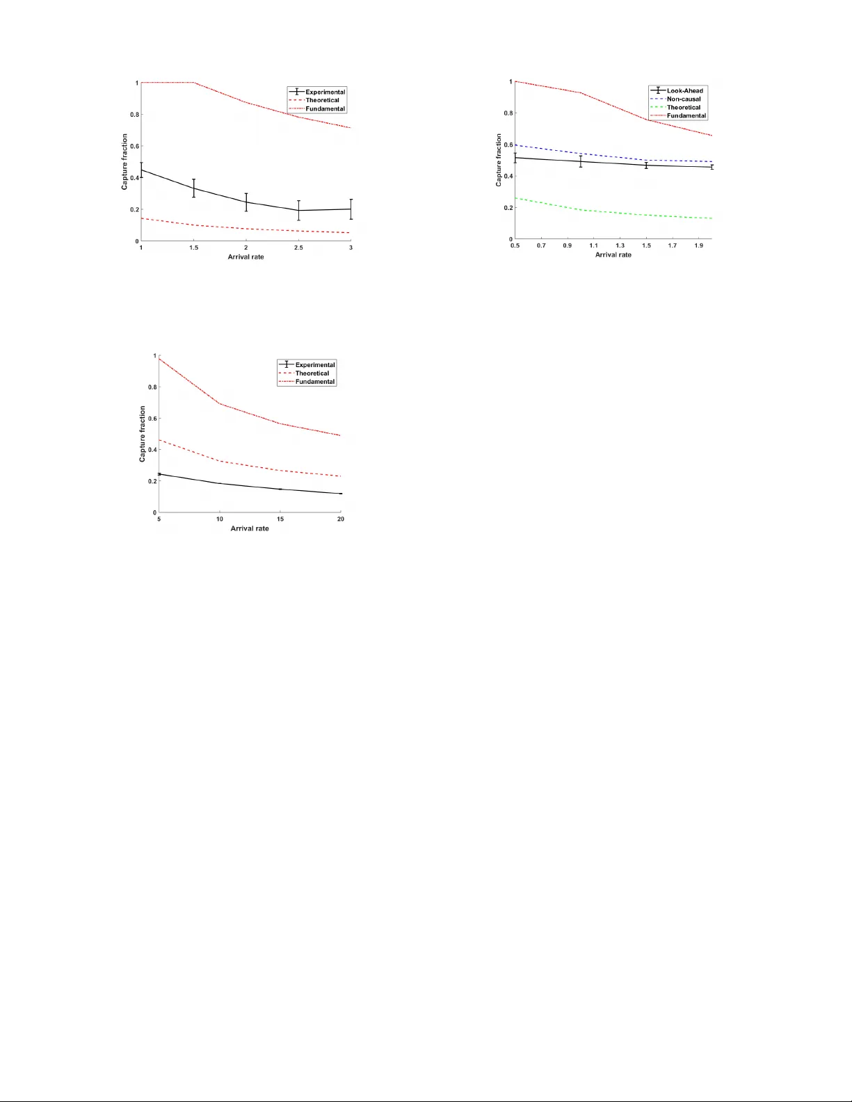
Dynamic Boundary Guarding Against Radially Incoming T argets Shi v am Bajaj and Shaunak D. Bopardikar Abstract — W e introduce a dynamic v ehicle routing pr oblem in which a single vehicle seeks to guard a circular perimeter against radially inward moving targets. T ar gets are generated uniformly as per a Poisson process in time with a fixed arrival rate on the boundary of a circle with a larger radius and concentric with the perimeter . Upon generation, each target moves radially inward toward the perimeter with a fixed speed. The aim of the vehicle is to maximize the capture fraction, i.e., the fraction of targets inter cepted bef ore they enter the perimeter . W e first obtain a fundamental upper bound on the capture fraction which is independent of any policy followed by the vehicle. W e analyze several policies in the low and high arrival rates of target generation. For low arrival, we propose and analyze a First-Come-First-Served and a Look- Ahead policy based on repeated computation of the path that passes through maximum number of unintercepted targets. For high arrival, we design and analyze a policy based on repeated computation of Euclidean Minimum Hamiltonian path through a fraction of existing targets and show that it is within a constant factor of the optimal. Finally , we provide a numerical study of the performance of the policies in parameter r egimes bey ond the scope of the analysis. I . I N T R O D U C T I O N Dynamic vehicle routing (D VR) problems are vehicle routing problems in which the vehicles have to plan their paths through the points of interest which arrive sequentially ov er time. This paper addresses a D VR problem in volving moving targets. T argets are generated at the boundary of an en vironment and mov e with a constant speed in order to enter a perimeter . A single vehicle is assigned a task of capturing as many targets as it can before they enter the perimeter . This setup is highly relev ant in surveillance applications that in volve gathering additional information on mobile targets and in civi lian space applications such as protecting the space-stations from debris. Additional applications of this setup are en visioned in guarding of airport runways from rogue drones. A. Related W ork Standard vehicle routing problems in operations research are concerned with planning optimal vehicle routes to visit a set of fixed targets. This requires solving an underlying combinatorial optimization problem [1]. In contrast, D VR requires that the vehicle routes be re-planned as ne w infor- mation becomes av ailable ov er time which was originally introduced on graphs in [2]. Fundamental limits, nov el policies and their constant factor optimality guarantees in continuous en vironments were established in [3]. Environ- ments may be dynamically varying [4], [5] and the targets The authors are with the Electrical and Computer Engineering Department, Michigan State Univ ersity , East Lansing, MI. Emails: bajajshi@msu.edu, shaunak@egr.msu.edu Fig. 1. Problem setup. The en vironment is an annulus of inner radius ρ and outer radius D . T argets are depicted as black dots approaching the perimeter at constant speed. The vehicle is shown as a triangle. may have multiple lev els of priorities [6] or can be randomly recalled [7]. The vehicles may be tasked with performing pickup and deliv ery operations [8],[9]; may possess motion constraints [10], [11], [12] and need not require mutual communication [13]. W e refer the reader to [14] for a revie w of this literature. There has been a recent research on pursuit of mobile targets that seek to reach a destination. In [15], the authors consider a setup of guarding a line segment in the case of a single pursuer and a single ev ader . They provide with different conditions in which either the defender or the attacker wins. The authors of [16] consider a pursuit ev asion dynamic guarding problem with two vehicles and one demand moving with constant speeds. The vehicles mo ve cooperativ ely to pursue the demand in a planar en vironment and giv es different cooperati ve strategy between the two pursuers. The same authors in [17] consider a differential game of attacker-tar get-defender . In [18], [19], the authors consider demands that are slo wer than the v ehicle which is moving parallel to x or y axis. Earlier, we introduced a D VR boundary guarding problem in which a single vehicle was assigned to stop the demands from reaching a deadline in a rectangular environment [20]. Our work [21] considered the case of tar gets being generated inside a disk-like en vironment and moving radially outward to escape the re gion. B. Contributions The en vironment considered in this paper is an annulus of inner radius ρ and outer radius D . The targets are generated uniformly and randomly on the boundary as per a Poisson process in time with rate λ . Upon generation, ev ery target mov es with a constant velocity v < 1 to wards the perimeter . A vehicle, modeled as a first-order integrator moving with unit speed, seeks to intercept the targets before they reach the perimeter . The performance of the vehicle is the expected value of the capture fraction, i.e., the fraction of the tar gets that are intercepted, at steady state. Our contrib utions are as follo ws. W e first determine a policy independent upper bound on the capture fraction of the targets and show that it scales as O ( 1+ v √ v λρ ) . Second, we design three policies for the vehicle and characterize analytic lower bounds on the resulting capture fraction in limiting parameter regimes. In particular , for lo w arriv al rates of the targets, we show that the capture fraction scales as Ω( 1 1+ λρ ) using a policy based on intercepting the targets as per the first-come-first-served order . W e then characterize the performance of a policy with look-ahead based on repeated computation of a path that maximizes the number of targets intercepted in a horizon. Third, in the regime of high arriv al rates λ → + ∞ , we analyze the performance of a policy based on repeated computation of the Euclidean Minimum Hamiltonian Path (EMHP) through the radially moving targets and show that its performance scales as Ω( 1 − v √ v (1+ √ v ) λρ ) . In particular , we show that the capture fraction of this polic y is within a constant factor of optimal if v → 0 + . Numerical simulations suggest that our analytic bounds generalize beyond the limiting parameter regimes. Although the focus of the problem is similar to the ones in [20] and in [21], the geometry of the environment and direction of the tar gets yield novel results. C. Or ganization The paper is organized as follows. Section II comprises the formal problem definition and a summary of background concepts and nov el intermediate properties. In Section III, we derive a nov el policy independent upper bound on the capture fraction. In Section IV, we present two policies suitable for low arriv al rate of the targets and we derive nov el lower bounds on their performance. In Section V, we present and analyze a policy suitable for high arriv al rates. In Section VI, we present results of numerical simulations. Finally , Section VII summarizes this paper and outlines directions for future research. I I . P R O B L E M F O R M U L A T I O N A N D P R E L I M I N A RI E S W e begin with a mathematical description of the problem and provide preliminary properties of the model considered. A. Mathematical Modeling and Pr oblem Statement Consider a disk like environment E = { ( r, θ ) : 0 < ρ ≤ r ≤ D , ∀ θ ∈ [0 , 2 π ) } . T argets appear uniformly and randomly at the boundary of the disk, i.e., at r = D . Upon generation, e very target mov es radially inward towards the inner circular boundary , termed as the perimeter , having radius ρ in E . The arriv al times of the targets are as per a Poisson process with rate λ . W e consider a single service vehicle with motion modeled as a first order integrator with unit speed and with the ability to mo ve in R 2 . The v ehicle is said to capture a target when it is collocated with a target while the target is in E . A target gets removed from the en vironment if it gets captured by the vehicle. A tar get is said to escape when it reaches the perimeter and is not intercepted by the vehicle. W e assume that the speed of the targets is less than that of the vehicle ( v < 1 ). Hence, a target must be captured within ( D − ρ ) /v time units of being generated. W e refer to this problem as RIT problem for conv enience. Let Q ( t ) ⊂ E denote the set of all outstanding target locations at time t . If the i th target that arriv es gets captured, then it is placed in Q capt ( t ) having cardinality n capt ( t ) , and is remov ed from Q ( t ) . Otherwise, it is placed in Q esc ( t ) ha ving cardinality n esc ( t ) and remov ed from Q ( t ) . Akin to our work in [20] that formally defined causal nature of policies, we will consider both causal and non-causal policies for the RIT problem, defined as follo ws. Causal P olicy: A causal feedback control policy for a vehicle is a map P : E × F → R 2 , where F ( E ) is the set of finite subsets of E , assigning a commanded velocity to the v ehicle as a function of the current state of the system, yielding the kinematic model, ˙ p ( t ) = P ( p ( t ) , Q ( t )) . Non-causal P olicy: In a non-causal feedback control polic y , the velocity of the vehicle is a function of current and future states of the system. Although these policies are physically unrealizable, they serve as a means to compare the performance of causal policies against the optimal. Pr oblem Statement: The aim of this paper is to design policies P that maximize the fraction of targets that are captured F cap ( P ) , termed as capture fraction , where F cap ( P ) := lim t →∞ sup E  n capt ( t ) n capt ( t ) + n esc ( t )  . In the sequel, we propose dif ferent policies that are suit- able for low and high arriv al rates of the targets. But we first present some preliminary and novel results in the next sub-section which will be used to establish the fundamental limit and analyze the policies. B. Pr eliminary Results W e revie w a concept related to longest paths on graphs as well as deri ve some basic results which will be used to obtain bounds on paths through a set of radially moving targets. 1) Longest P aths in Dir ected Acyclic Graphs (DA G): A graph G = ( V , E ) is called a directed graph if it consists of a set of vertices V and a set of directed edges E ⊂ V × V [20]. A graph is acyclic if its first and the last vertex are not same in the sequence. Finding the longest path, i.e. to find a path that visits maximum number of vertices, is NP-hard to solve as its solution requires the solution of Hamiltonian path problem [22]. Ho wev er, for a DA G, the longest path problem has an efficient dynamic solution, [23] with complexity that scales polynomially with the number of vertices. 2) Capturable set: The capturable set comprises the set of locations of all tar gets that can be captured from a gi ven vehicle location, defined formally as follows. Definition II.1 A vehicle located at ( x, 0) can captur e tar- gets located in the capturable set , C ( x, v , ρ ) := { ( r , θ ) ∈ E : r < r c , ∀ θ ∈ [0 , 2 π ) } wher e, r c ( x, v , ρ, θ ) = min { D , ρ + v p ρ 2 + x 2 − 2 xρ cos θ } . If the vehicle located at ( x, 0) requires time T to intercept a tar get located at ( r, θ ) , then r − v T ≥ ρ . By setting r c − v T = ρ , we obtain the expression for r c . The location r c corresponds to the location of the targets that the vehicle can capture before the y enter the perimeter . 3) Distribution of Outstanding T ar gets: In this subsection, we derive the distribution of targets in any region of the en vironment at steady state. Recall that an annular section A ( a, b, θ 1 , θ 2 ) ⊂ R 2 is the set A ( a, b, θ 1 , θ 2 ) := { ( r , θ ) | a ≤ r ≤ b, θ ∈ [ θ 1 , θ 2 ] } . Lemma II.1 (Outstanding targets) Suppose the arrival of tar gets starts at time 0 and no tar gets ar e intercepted in the interval [0 , t ] . Let Q denote the set of all targ ets in [ D , D − v t ] , ∀ θ ∈ [0 , 2 π ) at time t. Then, given a set R ( r , ∆ r, θ , ∆ θ ) , of infinitesimal area A , contained in Q , P [ | R ∩ Q | = n ] = e − ¯ λA ( ¯ λA ) n n ! , wher e ¯ λ = λ 2 π vr . Furthermor e, E [ | R ∩ Q | ] = ¯ λr ∆ r ∆ θ , and V ar [ | R ∩ Q | ] = ¯ λr ∆ r ∆ θ . Pr oof: Let R ( r, ∆ r , θ , ∆ θ ) ⊂ R 2 be an area element where ∆ r , ∆ θ are infinitesimally small. Let Q denote the set of all targets in [ D , D − v t ] , ∀ θ ∈ [0 , 2 π ) . Then, the probability that R contains n points out of Q at time t satisfies P [ |R ∩ Q| = n ] = ∞ X i = n P [ i targets arriv e in [ D − ( r + ∆ r ) v , D − r v ] × P [ n of i targets generated in ( θ , θ + ∆ θ )] . Since the generation is uniform in space and Poisson in time, P [ i targets arriv e in [0 , ∆ r v ]] = e ( − λ ∆ r v ) ( λ ∆ r v ) i i ! , and P [ n of i tar gets generated in (0 , ∆ θ )] =  i n   ∆ θ 2 π  n  1 − ∆ θ 2 π  i − n . Let ∆ r /v = R and ∆ θ / 2 π = H . Thus, P [ | R ∩ Q | = n ] = ∞ X i = n e − λR ( λR ) i i ! ( i !)( H ) n (1 − H ) i − n ( n !)( i − n )! = e − ¯ λA ( ¯ λA ) n n ! , Fig. 2. The quantity T i +1 indicates the time taken by the vehicle to mov e from target i to the target i + 1 . where ¯ λ = λ/v 2 πr and A is the area of the annulus sector . This result establishes that the number of unintercepted targets in an annulus is Poisson distributed uniformly with parameter λ v ∆ d , where ∆ d is the difference in the radii of the annulus. 4) Bounds on paths thr ough static and incoming tar gets: The following result will be used to bound the length of the path through targets in the en vironment. Lemma II.2 (Bounds on path through incoming targets) Let T be the length of the actual path through the incoming tar gets and T s be the length of the path thr ough their static initial locations. Then, T s 1 + v ≤ T ≤ T s 1 − v . Pr oof: Let the targets be labeled in the order in which they arri ve. Let T j be the time taken by the vehicle to capture the j th incoming target. Consider the i th target at ( r i , θ i ) . The vehicle will capture this target at time P i j =1 T j . It then mov es toward the ( i + 1) th target and reaches it in a time duration of T i +1 which is equal to the distance covered due to unit speed. Let the distance between ( r i − v P i +1 j =1 T j , θ i ) and ( r i +1 − v P i +1 j =1 T j , θ i +1 ) be T 0 i +1 . Also, let T s,i +1 be the distance between ( r i − v ¯ T , θ i ) and ( r i +1 − v ¯ T , θ i +1 ) , where ¯ T < T . As the distance between two targets moving radially inward with same speed is non-increasing function of time, T s,i +1 ≤ T 0 i +1 . Therefore, from triangle inequality (Fig. 3), T i +1 + v T i +1 ≥ T 0 i +1 . This means, T i +1 ≥ T 0 i +1 / (1 + v ) ≥ T s,i +1 / (1 + v ) . Extending this to all the tar gets we get the expression, T = P n i =1 T i +1 ≥ P n i =1 T s,i +1 1+ v = T s 1+ v . The proof for the upper bound is similar to the proof abo ve and has been omitted for brevity . Next we revie w classic results regarding the upper bound on the length of the shortest path through a set of fixed points in an environment. Lemma II.3 (Shortest Euclidean path [24]) Given n points in a squar e of length R , ther e is a path thr ough the n points of length not e xceeding R √ 2 n + 1 . 75 R . Fig. 3. (a) The set S T for RIT problem. The set ¯ S T is shown by a solid boundary , which is a circle of radius (1 + v ) T . (b) The area element ζ of length and width m in ¯ S T . Lemma II.4 (Length of EMHP tour [25]) Consider a set Q of n points independently and uniformly distributed in a compact set A of area |A| . Then, ther e exists a constant β T S P such that, lim n →∞ ` ( E M H P ( Q )) √ n = β T S P p |A| , with pr obability one. The constant β T S P has been estimated numerically as β T S P ≈ 0 . 7120 ± 0 . 0002 . I I I . A P O L I C Y - I N D E P E N D E N T U P P E R B O U N D This section summarizes the first of our analytic results – a policy independent upper bound on the capture fraction. This is a fundamental limit to this problem and is valid for any values of the problem parameters. First, we deri ve a lower bound on the expected travel time between two targets, and will be used to derive the fundamental bound. Lemma III.1 (T ravel time lower bound) If T d is a ran- dom variable denoting the time r equir ed to travel between tar gets in Q , then E [ T d ] ≥ 1 1 + v r v πρ 2 λ . Pr oof: Let S T comprise the set of targets that can be reached from vehicle position ( X, 0) in at most T time units, as shown in Fig. 3. Mathematically , S T := { ( r , θ ) ∈ E | X 2 +( r − vT ) 2 − 2 X ( r − v T ) cos θ ≤ T 2 } . Also, let ¯ S T := { ( r , θ ) ∈ E | ( X − r cos θ ) 2 +( r sin θ ) 2 ≤ ((1+ v ) T ) 2 } . Since the relati ve v elocity of any target with respect to the vehicle is less than or equal to (1 + v ) , the distance d 1 of any point on the boundary of S T from ( X, 0) is at most T (1 + v ) . This means that the set S T will be contained in a circle centered at the same position ( X , 0) of radius (1 + v ) T , i.e., S T ⊂ ¯ S T . If T d denotes the minimum amount of time needed to go from vehicle location ( X, 0) to any target, then, T d > T , if S T is empty i.e., P [ T d > T ] = P [ | S T | = 0] . Moreov er , P [ | ¯ S T | = 0] = P [ | S T | = 0] P [ | ¯ S T \ S T | = 0] ≤ P [ | S T | = 0] . Now , consider an infinitesimal area element ζ of length and width m at ( s, 0) from the center (cf. Fig. 3 (b)). From Lemma II.1, the probability that ζ is empty will be: P [ | ζ | = 0] = e − λ 2 πv dθdr = e − λ 2 πv m 2 s ≥ e − λm 2 2 πv ρ = e − λ 2 πv ρ Area( ζ ) , where the inequality comes from the fact that s ∈ [ ρ, D ] . Since every compact set can be written as a countable union of non-overlapping area elements, the result is true for ¯ S T as well. Therefore, P [ | S T | = 0] ≥ P [ | ¯ S T | = 0] ≥ e − λ 2 vρ ((1+ v ) T ) 2 , and thus, the e xpectation of T d can be bounded as E [ T d ] = Z ∞ 0 P [ T d > T ] dT = Z ∞ 0 P [ | S T | = 0] dT ≥ Z ∞ 0 P [ | ¯ S T | = 0] dT = √ π 2(1 + v ) r 2 v ρ λ = 1 1 + v r π vρ 2 λ . W e now present the main result of this section. Theorem III.1 (Upper bound on capture fraction) Any policy P for the RIT pr oblem must satisfy F cap ( P ) ≤ min ( 1 , (1 + v ) r 2 v λπρ ) . Pr oof: T o service a fraction c ∈ (0 , 1] of targets, the service rate of the targets must be greater than the arriv al rate [26], i.e., cλ E [ T d ] ≤ 1 . Using Lemma III.1, we obtain this result. W ith this fundamental limit in place, we will now present sev eral policies and examine their performance in compari- son to this upper bound. I V . L OW A R R I V A L R AT E O F T A R G E T S W e propose two main policies for the parameter regime of low arriv al rates of targets. The FCFS policy is very simple to implement whereas the look ahead (LA) policy requires repeated computation of longest paths. A. F irst-Come-F irst-Serve (FCFS) policy According to this policy , the vehicle intercepts the targets in the order in which they arriv e. If there are no outstanding targets, the vehicle waits at the center of E for the targets to appear . The policy is summarized in Algorithm 1. Algorithm 1: First-Come-First-Serve (FCFS) polic y 1 Assumes that the vehicle is at the center . 2 if No outstanding targ ets in E then 3 W ait for the next target to arrive, 4 else 5 Mov e to intercept the target farthest from the boundary . 6 end 7 Repeat. Theorem IV .1 (FCFS capture fraction) F or any v ∈ [0 , 1) , λ ≥ 0 , the captur e fraction of the FCFS policy satisfies F cap ( FCFS ) ≥ 1 1 + 2 λρ . Pr oof: F or n capt ( t ) > 0 at some t > 0 , F cap = lim t → + ∞ sup E   1 1 + n esc ( t ) n capt ( t )   ≥  1 + lim t → + ∞ sup E  n esc ( t ) n capt ( t )  − 1 where the last inequality comes from an application of Jensen’ s inequality applied to the conv ex function, 1 (1+ x ) [27]. Thus, by quantifying the expected number of targets that escape per tar gets captured, we can determine a lower bound on the capture fraction. The FCFS policy is difficult to analyze directly . Thus, we provide the lower bound by analyzing an even simpler Stay- at-Center (SA C) policy in which the vehicle captures a target just before the target enters the perimeter and returns back to the center . Consider a target i within the capturable set of the vehicle. The time taken by the v ehicle to capture the target just before the perimeter and return back to the center will be 2 ρ . Thus, the number of targets that can breach the perimeter will be equal to the number of targets that enter the capturable set while the vehicle is capturing the i th target, i.e., all the targets that are at a distance of 2 ρv from the capturable set. Thus, from Lemma II.1, the expected number of targets that will escape is 2 λρ and the result follows. B. P olicies based on Look-ahead W e now propose and analyze a class of policies in which we constrict the movement of the vehicle such that the vehicle can only move along the perimeter . While such a motion may be sub-optimal in the present context, it allows us to leverage tools from graph theory and adapt our earlier ideas on longest path through the mobile targets to design efficient policies [20]. Definition IV .1 (Reachable targets) A targ et located at ( r , θ ) is reachable from the vehicle location ( ρ, φ ) if r − ρ ≥ v | θ − φ | ρ, for any v ∈ [0 , 1) . Definition IV .2 (Reachable set) The reac hable set fr om the vehicle position ( ρ, φ ) ∈ E is R ( ρ, φ ) := { ( r, θ ) ∈ E : r − ρ ≥ v | θ − φ | ρ } . This means that a target is reachable if it lies in R ( ρ, φ ) . Next, we define the notion of a reachability graph ov er the set of radially incoming targets that is inspired out of a similar construction in [20]. Definition IV .3 (Reachability graph) A r eachability graph of a set of points { ( r 1 , θ 1 ) , . . . , ( r n , θ n ) } ∈ E , is a DA G with vertex set V := { 1 , ...n } , and edge set E wher e, for j , k ∈ V and r j < r k , the edge ( j, k ) is in E if and only if ( r k − ( r j − ρ ) , θ k ) ∈ R ( ρ, θ j ) . W e now define a policy based on look-ahead wherein the vehicle computes the longest path in the reachability graph of all the targets in E and captures them on the perimeter . Algorithm 2 describes the algorithm for Look Ahead policy . Algorithm 2: Look Ahead (LA) polic y 1 Assumes that v ehicle is located on the perimeter . 2 Compute the reachability graph of all the targets in Q (0) and the v ehicle position. 3 Compute the longest path in this graph, starting from the vehicle position. 4 Capture targets in the order they appear at the perimeter . 5 Repeat; Akin to the rectangular environment considered in [20], Algorithm 2 is dif ficult to analyze directly . Instead, we design a Non-causal Look Ahead (NCLA) policy . In this policy , at time 0 , the vehicle computes a reachability graph, from its current position using the information of all the future targets that are yet to arrive in E . The vehicle then computes the longest path and captures the targets in the order in which they appear in that path. The algorithm for NCLA policy is formalized in Algorithm 3. Algorithm 3: Non-causal Look Ahead (NCLA) policy 1 Assumes that v ehicle is located on the perimeter . 2 Compute the reachability graph of all the targets in Q (0) ∪ Q unarr ived (0) and the v ehicle position. 3 Compute the longest path in this graph, starting from the vehicle position. 4 Capture targets in the order they reach the perimeter . The follo wing result provides a guarantee on the performance of the LA polic y relativ e to the NCLA. Theorem IV .2 (LA policy) If D − ρ ≥ v π ρ , then the captur e fr action of the LA policy satisfies F cap ( LA ) ≥  1 − v πρ D − ρ  F cap ( NCLA ) . Pr oof: [Sketch] Let the generation of targets begin at t = 0 and consider two scenarios; (a) Look ahead polic y is used by the vehicle, and (b) the vehicle uses the Non-causal look ahead policy (Fig. 4). Then, akin to the steps in the proof of Theorem IV.6 of [20], we can compare the number of targets captured in both the scenarios. Consider a time instant t 1 where the vehicle is computing the path through all outstanding targets Q ( t 1 ) and denote the path by Π a ( t 1 ) . The path in scenario (b), denoted as Π b ( t 1 ) , that the v ehicle will take through Q ( t 1 ) be giv en by (( r 1 , θ 1 ) , ( r 2 , θ 2 ) . . . , ( r m , θ m )) ∈ Q ( t 1 ) . The Fig. 4. Scenarios for proof of Theorem IV .2. In (a), vehicle visits 5 targets so L a = 5 .(b) vehicle visits 6 targets so m = 6 . ( r 2 , θ 2 ) is the highest target on (b) capturable from p a ( t 1 ) thus n = 1 . The red line shows the path followed by the vehicle in NCLA through arrived and unarri ved targets. target ( r 1 , θ 1 ) is reachable from Π b ( t 1 ) , but might not be reachable from Π a ( t 1 ) . The path Π a ( t 1 ) comprises tar gets: (( r n +1 , θ n +1 ) , ( r n +2 , θ n +2 . . . , ( r m , θ m )) , n ∈ { 0 , ..., m − 1 } , where ( r n +1 , θ n +1 ) is the highest target that is reachable from Π a ( t 1 ) . Thus, the length of Π a ( t 1 ) will satisfy L a ≥ m − n , where m is the length of the path in (b) because the edge weights of the DA G equal unity . Since the worst-case location for the vehicle is when it is diametrically opposite to the incident tar get direction, the v ehicle can capture an y target i if v π ρ + ρ ≤ r i . T argets at ( r 1 , θ 1 ) , . . . , ( r n , θ n ) must be at least v π ρ + ρ from the center . If N tot is the total number of outstanding targets in E at time t 1 , then by Lemma II.1 E [ n | N tot ] = N tot v πρ D − ρ F cap ( NCLA ) . Similarly , in scenario (b), E [ m | N tot ] = N tot F cap ( NCLA ) . Therefore, using the fact that L a ≥ m − n , E [ L a N tot | N tot ] ≥ 1 − v πρ D − ρ ! F cap ( NCLA ) . The ratio L a / N tot is the fraction of outstanding targets from the set Q ( t 1 ) that will be captured in scenario (a) and the ratio does not depend on N tot . Thus, by law of total expectation, we get obtain the desired claim. In Theorem IV .2, we established the performance of the LA policy relati ve to NCLA policy . Howe ver , we can also provide an explicit lo wer bound on the capture fraction for the LA policy , as summarized in the result belo w . Theorem IV .3 (Explicit LA captur e fraction) If D − ρ ≥ v πρ , then the LA policy satisfies F cap ( LA ) ≥ 1 π √ λρ erf ( √ λπ ρ ) + e − λπ ρ , wher e erf : R → [ − 1 , 1] is the err or function. Pr oof: The central idea is to construct an in vertible transformation between an y realization of targets and the vehicle in E to a rectangular environment akin to the problem Fig. 5. The transformation of the environment from a disk like to a rectangle. considered in [20]. W e then use the analysis from Theorem IV .8 from [20] to arrive at this claim. Consider an en vironment E 1 that can be constructed by cutting along the radius of E as illustrated in Fig. 5. The transformed environment E 1 is an isosceles trapezoid with the two parallel sides equal to 2 π D and 2 π ρ respectiv ely . In en vironment E 1 , the transformed targets move from an initial point on the longer side tow ard the corresponding point on the smaller side so that the time taken by every target to reach the smaller side is the same for all targets. This can be achiev ed by scaling the speed of each target appropriately as a function of the initial location of the target. E 1 can further be transformed to a rectangular en vironment E 2 in which the transformed targets mov e from an initial point on the lower edge toward the upper edge with equal speeds. Mathematically , consider a target located at ( r, θ ) in E . This means that the tar get is r − ρ distance away from the perimeter . Thus, in E 2 , the target will be r − ρ distance aw ay from the upper edge. Similarly , the target will be at a distance of θ ρ from one of the sides in E 2 . Thus, the location of the transformed target in E 2 will be ( θ ρ, r − ρ ) . Similarly , if the vehicle is located at ( ρ, φ ) and constricted to move on the perimeter , its location after transformation in E 2 will be φρ distance away from one of the side and on the upper edge as in E 1 and captures targets as per Algorithm 2. Thus, given any location of the vehicle on the perimeter and any set of locations of targets in E , we can construct a corresponding vehicle location on the upper edge and a set of locations of corresponding tar gets in E 2 such that the number of tar gets intercepted by the vehicle in the E and E 2 is equal. Then, the capture fraction of the LA policy applied to the RIT problem in en vironment E is lower bounded by the LA policy applied to the transformed problem in en vironment E 2 . In particular , the LA policy is expected to perform better because of the circular symmetry of E that allows the vehicle in E to reach certain tar gets in a shorter duration. This completes the proof. Note that the capture fraction of LA policy in Theorem IV .3 is independent of v . Furthermore, the capture fraction of FCFS policy presented in this section performs well for low arriv al rates, i.e., F cap ( FCFS ) → 1 for λ → 0 , but not in high arriv al regime since the upper bound scales as O (1 / √ λ ) . W e seek an improved policy in this regime which is the focus of the next section. Fig. 6. The RMHP-fraction policy . The figure on the left sho ws the EMHP through all outstanding targets. The figure on the right shows the instant when the vehicle has followed the path through ρ/v time units and allows some targets to escape. V . H I G H A R R I V A L R AT E O F T AR G E T S W e no w introduce a policy based on repeated computation of the EMHP through outstanding radially moving targets. W e term this polic y as the Radial Minimum Hamiltonian P ath (RMHP) policy . The key idea is that the number of targets accumulating near the perimeter is high. Thus, the time taken by the vehicle to capture successive tar gets will be small, and therefore, the vehicle can capture a lar ge number of targets in a single iteration. The vehicle uses solution of the EMHP path (i.e., a path that visits all the points exactly once) to determine the order of the targets to capture. In particular , we consider a constrained EMHP problem which starts at a specific point while visiting all the gi ven set of points [20]. The RMHP-fraction policy is defined in Algorithm 4. In this policy , the vehicle computes the EMHP path through all outstanding targets in (2 ρ, 3 ρ ) for all θ ∈ [0 , 2 π ) (Fig.6). The vehicle captures the targets for ρ v time units and then recomputes the EMHP path through the outstanding targets, allowing the remaining tar gets in that batch to escape. Algorithm 4: RMHP-fraction policy 1 Assumes that vehicle is located at a distance of 2 ρ from the origin. 2 Compute an EMHP path through the outstanding targets located at distance between 2 ρ and 3 ρ from the origin. 3 if time to travel entire path is less than ρ v then 4 Capture all the outstanding targets by follo wing the computed path. 5 else 6 Capture the targets in the order given by the EMHP . 7 end 8 Repeat from step 2. Theorem V .1 ((RMHP-fraction capture fraction) In the limit as λ → + ∞ , the capture fr action of the RMHP-fraction policy , with probability one is F cap (RMHP-fraction) ≥ min ( 1 , 1 − v α p v λρ (1 + √ v ) ) , where α = 6 √ 2 . Pr oof: Consider the beginning of an iteration of the policy and assume that the duration of the previous iteration was ρ/v time units. At this instant, the vehicle will be 2 ρ distance away from the center and suppose there are n outstanding targets in an annulus of radii 2 ρ and 3 ρ . From Lemma II.2 and Lemma II.3, the length of the tour through these targets can be upper bounded by αρ √ n/ (1 − v ) where, α = 6 √ 2 . As the v ehicle can capture targets for at most ρ v time units, it will capture cn targets, where c = min ( 1 , ρ/v ( ρα √ n ) / (1 − v ) ) = min ( 1 , 1 − v v α √ n ) . From Lemma II.1, the expected value E [ n ] and the v ariance σ 2 n of the random variable n is λρ v . Using Chebyshev inequality , P [ | n − E [ n ] | ≥ γ ] ≤ σ 2 n /γ 2 , and γ = √ v E [ n ] , P [ n ≥ (1 + √ v ) E [ n ]] ≤ 1 v E [ n ] = 1 λρ . Thus, we have c ≥ min ( 1 , 1 − v α p v λρ (1 + √ v ) ) with probability at least 1 − 1 λρ . Corollary V .1 (Constant factor of optimality:) F or v → 0 + and λ → + ∞ , the capture fraction c ≥ min ( 1 , 1 α √ v λρ ) , which is within a constant of 12 / √ π ≈ 6 . 77 . Using Lemma II.4, we obtained a better bound on the length and thus a better constant factor of optimality . Corollary V .2 (Improv ed constant factor of optimality:) F or v → 0 + and λ → + ∞ , the capture fraction c ≥ min ( 1 , 1 α √ v λρ ) , which is within a constant of 3 . 988 / √ π ≈ 2 . 25 . V I . S I M U L A T I O N S W e no w present results of numerical experiments for the policies analyzed in Sections IV and V. The parameters D = 20 and ρ = 3 were kept fixed. The first result compares the FCFS policy to the lower and fundamental bounds. Comparison of the LA policy to the NCLA polic y and to the theoretical bounds is sho wn in the second result. Finally , the last result compares the RMHP-fraction policy to the theoretical bounds. For the FCFS policy , we simulated 30 runs for each arriv al rate. Fig. 7 shows a comparison of the FCFS polic y with the theoretical bounds. T o simulate the NCLA and LA policies, we implement 5 runs for each value of the arriv al rate. Fig. 9 shows the comparison of the LA policy with NCLA, fundamental and theoretical bounds. T o simulate Fig. 7. Simulation results for FCFS. Comparison of FCFS policy with fundamental and theoretical bounds for v=0.2. The red dash-dot line shows the fundamental upper bound and red dash curve shows the theoretical bound for FCFS. Fig. 8. Simulation results for RMHP-fraction policy for v=0.04. The red dash-dot curve is from the policy independent upper bound in Theorem III.1 and the dashed curve shows the theoretical bound. the RMHP-fraction policy , the linkern 1 solver was used. For each value of the arriv al rate, 5 runs of the policy was taken. The comparison is shown in Fig. 8. Note that the experimental results for RMHP-fraction policy are lower than the theoretical lower bound in Theorem V .1. This is because we have not reached the limit as v → 0 + and λ → + ∞ . Moreov er , we utilize an approximate solution for the EMHP generated by the linkern solver . V I I . C O N C L U S I O N S A N D F U T U R E W O R K This paper introduced the RIT problem, in which a vehicle seeks to defend a perimeter from the radially inward moving targets. W e established a policy independent upper bound on the capture fraction of the targets. W e then proposed three different policies suitable for low and high arri v al rates of the targets and analyzed their respectiv e capture fractions. In the case of low arri val rate of targets, we proposed FCFS, and LA policies. For the latter case, we introduced the RMHP- fraction policy which is within a constant f actor of optimal. This problem can be extended in many ways. One can consider the case when the speed of the targets is not 1 The TSP solver linkern is freely av ailable for academic research use at http://www.math.uwaterloo.ca/tsp/concorde/ . Fig. 9. Simulation results for NCLA and LA policy for v=0.8. The red curve shows the fundamental upper bound. Capture fraction of NCLA is shown by the blue curve and the theoretical bound analyzed in IV .2 is shown in green color . constant or the targets can maneuver away from the vehicle to escape. Other extensions include multi-vehicle versions of this problem. R E F E R E N C E S [1] P . T oth and D. V igo, “ An overview of vehicle routing problems, ” in The vehicle routing pr oblem . SIAM, 2002, pp. 1–26. [2] H. N. Psaraftis, “Dynamic vehicle routing problems, ” V ehicle r outing: Methods and studies , vol. 16, pp. 223–248, 1988. [3] D. J. Bertsimas and G. V an Ryzin, “Stochastic and dynamic vehicle routing in the euclidean plane with multiple capacitated vehicles, ” Operations Researc h , vol. 41, no. 1, pp. 60–76, 1993. [4] J. D. Papasta vrou, “ A stochastic and dynamic routing policy using branching processes with state dependent immigration, ” European Journal of Operational Researc h , vol. 95, no. 1, pp. 167–177, 1996. [5] M. Pavone, E. Frazzoli, and F . Bullo, “ Adapti ve and distributed algo- rithms for vehicle routing in a stochastic and dynamic environment, ” IEEE T rans. on Auto. Cont. , vol. 56, no. 6, pp. 1259–1274, 2011. [6] S. L. Smith, M. Pav one, F . Bullo, and E. Frazzoli, “Dynamic vehicle routing with priority classes of stochastic demands, ” SIAM Journal on Contr ol and Optimization , vol. 48, no. 5, pp. 3224–3245, 2010. [7] S. D. Bopardikar and V . Sriv astav a, “Dynamic vehicle routing in presence of random recalls, ” IEEE Control Systems Letters , 2020, to appear . [8] H. A. W aisanen, D. Shah, and M. A. Dahleh, “ A dynamic pickup and deliv ery problem in mobile networks under information constraints, ” IEEE T rans. on Auto. Cont. , vol. 53, no. 6, pp. 1419–1433, 2008. [9] K. Treleav en, M. P av one, and E. Frazzoli, “ Asymptotically optimal algorithms for one-to-one pickup and delivery problems with appli- cations to transportation systems, ” IEEE Tr ansactions on Automatic Contr ol , vol. 58, no. 9, pp. 2261–2276, 2013. [10] K. Savla, E. Frazzoli, and F . Bullo, “T rav eling salesperson problems for the dubins vehicle, ” IEEE T ransactions on Automatic Contr ol , vol. 53, no. 6, pp. 1378–1391, 2008. [11] K. Savla, F . Bullo, and E. Frazzoli, “T rav eling salesperson problems for a double integrator , ” IEEE T ransactions on Automatic Contr ol , vol. 54, no. 4, pp. 788–793, 2009. [12] S. Itani, E. Frazzoli, and M. A. Dahleh, “Dynamic traveling repair- person problem for dynamic systems, ” in 2008 47th IEEE Conference on Decision and Control . IEEE, 2008, pp. 465–470. [13] A. Arsie, K. Savla, and E. Frazzoli, “Efficient routing algorithms for multiple vehicles with no explicit communications, ” IEEE T ransac- tions on Automatic Contr ol , vol. 54, no. 10, pp. 2302–2317, 2009. [14] F . Bullo, E. Frazzoli, M. Pav one, K. Savla, and S. L. Smith, “Dynamic vehicle routing for robotic systems, ” Pr oceedings of the IEEE , vol. 99, no. 9, pp. 1482–1504, 2011. [15] P . Kawecki, B. Kraska, K. Majcherek, and M. Zola, “Guarding a line segment, ” Systems and Contr ol Letters , vol. 58, pp. 540–545, 2009. [16] Z. E. Fuchs, E. Garcia, and D. W . Casbeer, “T wo-pursuer, one-ev ader pursuit ev asion differential game, ” in NAECON 2018-IEEE National Aer ospace and Electr onics Confer ence . IEEE, 2018, pp. 457–464. [17] E. Garcia, D. W . Casbeer , and M. Pachter, “Optimal target capture strategies in the target-attacker -defender differential game, ” 06 2018, pp. 68–73. [18] P . Chalasani and R. Motwani, “ Approximating capacitated routing and delivery problems, ” SIAM J. Comput. , vol. 28, no. 6, pp. 2133–2149, Aug. 1999. [Online]. A vailable: https://doi.or g/10.1137/ S0097539795295468 [19] S. D. Bopardikar, S. L. Smith, F . Bullo, and J. P . Hespanha, “Dy- namic vehicle routing for translating demands: Stability analysis and receding-horizon policies, ” IEEE T ransactions on Automatic Contr ol , vol. 55, no. 11, pp. 2554–2569, 2010. [20] S. L. Smith, S. D. Bopardikar, and F . Bullo, “ A dynamic boundary guarding problem with translating targets, ” in Decision and Contr ol, 2009 held jointly with the 2009 28th Chinese Contr ol Conference. CDC/CCC 2009. Pr oceedings of the 48th IEEE Conference on . IEEE, 2009, pp. 8543–8548. [21] P . Agharkar , S. D. Bopardikar, and F . Bullo, “V ehicle routing algo- rithms for radially escaping targets, ” SIAM Journal on Contr ol and Optimization , vol. 53, no. 5, pp. 2934–2954, 2015. [22] B. Korte, J. Vygen, B. K orte, and J. Vygen, Combinatorial optimiza- tion . Springer , 2012, vol. 2. [23] N. Christofides, Graph Theory: An Algorithmic Approac h (Computer Science and Applied Mathematics) . Orlando, FL, USA: Academic Press, Inc., 1975. [24] L. Few , “The shortest path and the shortest road through n points, ” Mathematika , vol. 2, no. 2, p. 141144, 1955. [25] J. Beardwood, J. H. Halton, and J. M. Hammersley , “The shortest path through many points, ” Mathematical Proceedings of the Cambridge Philosophical Society , vol. 55, no. 4, p. 299327, 1959. [26] L. Kleinrock, Theory , V olume 1, Queueing Systems . Ne w Y ork, NY , USA: W iley-Interscience, 1975. [27] Z. Cvetko vski, Con vexity , Jensen’ s Inequality . Berlin, Heidelberg: Springer Berlin Heidelberg, 2012, pp. 69–77. [Online]. A vailable: https://doi.org/10.1007/978- 3- 642- 23792- 8 7