Sensor Switching Control Under Attacks Detectable by Finite Sample Dynamic Watermarking Tests

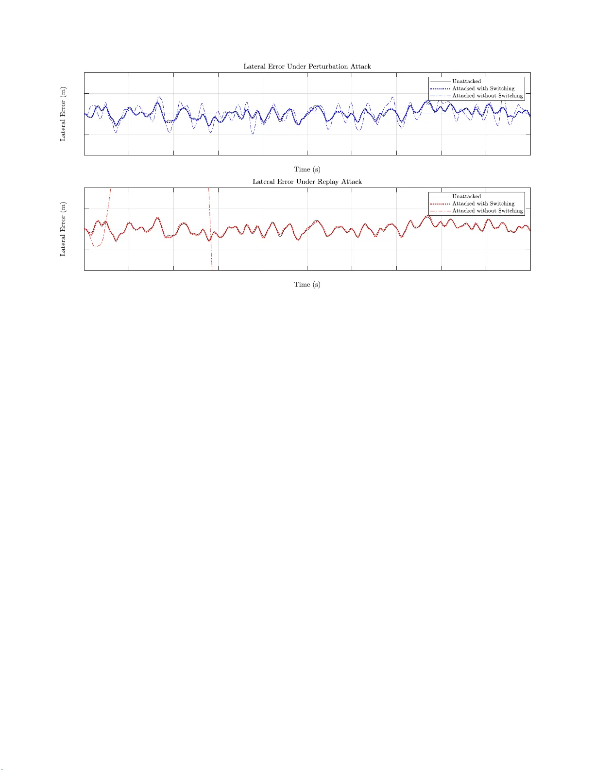
1 Sensor Switching Control Under Attacks Detect able by Finite Sample Dynamic W aterma rking T ests Pedro Hespan h ol, Matt hew Porter , Ram V asudevan, and Anil As wani Abstract —Control system security is enhanced by the ability to detect malicious attacks on sensor measurements. Dynamic watermarking can detect such attacks on linear ti me-inva riant (L TI) systems. Ho wev er , existing theory f ocuses o n attack detec- tion and not on the use of watermarking in conjunction with attack mitigation strategies. In this paper , we study th e problem of switching b etween tw o sets of sensors : One set o f sensors h as high accuracy but is vulnerable to attack, while the second set of sensors h as low accuracy but cannot be attacked. The p roblem is to design a sensor switching strategy based on attack d etection by dynamic watermarking. This requires new theory because existing results are not adeq u ate to control or bound the behavior of sen sor switching strategies th at use finite data. T o ov ercom e this, we develo p new finite sample hypothesis tests for dynamic watermarking in the case of b ounded disturbances, using the modern t heory of concentration of measure for random matrices. Our resulting switching st rategy is validated with a simu l ation analysis in an autonomous driving setti ng, whi ch demonstrates the strong perform ance of our proposed policy . Index T erms —Dynamic watermarking, observer switching con- trol, finite sample tests I . I N T R O D U C T I O N T HE secu re and resilien t contro l o f cyber-physical systems (CPS) require s safe opera tion in the face of maliciou s attacks that can occur on either the physical layer (e.g., sensors and actuators) o r the cybe r layer (e.g., communica- tion a n d co mputation cap abilities)[1]. Real-life inciden ts like the Maroo c h y-Shire in cident [2], the Stuxnet worm [3], and others [4] illustrate the importan c e of concerns about CPS security . One approach to secure contro l has been to focus on cybersecurity of CPS [5], [6], [ 7], [ 8], but this does no t fully exploit the phy sical asp ects o f CPS. An altern ati ve is attack identification and detectio n considerin g the interplay between the cyber and physical parts of CPS [9], [4], [10], [ 11]. M any of these techniques are static (i.e., do n ot consider system dynamics) [12] or passi ve (i.e., do not actively control system to id entify maliciou s nodes and senso rs) [13], [14], [1 5]. In contrast, dynamic w atermarking is an acti ve defense technique that injects per turbation s in to the system contr ol in order to detect attacks [1 6], [17], [ 18], [19]. More specifically , this method applies a private excitation to the sy stem, wh ich This work wa s supported by the UC Berkele y Center for L ong-T erm Cybersec urity , and by a grant from Ford Motor Co mpany via the Ford-UM Allianc e under award N022977. Pedro Hespanhol and Anil Aswani are with the Department of In- dustrial Engineering and Operations Researc h, Uni versi ty of California, Berk ele y , CA 94720, USA pedrohespanhol@ berkeley.edu, aaswani@berke ley.edu Matthe w Porter and Ram V asude va n are with the Departmen t of Me- chanic al Engineering, Univ ersity of Michiga n, Ann Arbor , MI 48109, USA matthepo@umic h.edu, ramv@umich.edu is a disturban ce o nly known to th e contro ller . T h en it uses consistency tests to detec t attacks by check ing for correlatio n between sen sor measur ements and the p riv ate excitation. The goal is to be able to d etect all sensor attacks whose magnitud e exceeds some prespecified amo unt. A. Asymptotic R e sults for Dynamic W atermarking Research on d ynamic watermarkin g can be di vided into two main areas o f contribution: The first is the development of statistical hypoth esis testing that tries to detect corrupted mea- surements by ob serving co r relations between sensor outputs and the dynam ic watermark [17], [20], [1 8], [16], [21]. T h is set of techn iques apply to gener a l L TI systems, b ut can not ensure the zero-average-power property for general attack mode ls. The second line of work [ 22], [23] c o nsiders g eneral attack models and d ev elop tests able to en sure that only attacks which add a zero-average-power signal to the sensor measur e ments can remain und etected, but constrain their analysis to L TI systems with specific structure o n their dynam ics. More recently , Th e work done in [24] and [ 25] attempts to bridge this g ap by p r oviding statistical guar antees for complex types o f attacks for gener al L TI systems. While both pap ers address a genera l MIMO L TI system , the set of assum ptions are som ewhat different: the former assumes o pen-loo p stability of the L TI system, and the latter restricts the attack form. In particular, in [ 25], the tests provided are able to d e te c t if a gen eral MIMO L TI system is under a fairly gene r al type of attack. In par ticular , it consid e r s add itiv e attack s that can dampen/amplify the system m easurements, can replay the system from a d ifferent initial condition , or can do both. This form of attack, while arguably simple, encomp asses many of the types of attacks reported in real-life incidents (e.g., replay attacks [3 ]) as well as compen sate for external disturban ces not accounted b y the system mo del (e.g ., wind when represented via intern al mod el princip le [25]). W e proceed to briefly summar ize the results of [25], as it is the fo undatio n for this curr ent paper . Consider a MI MO L TI system with partial observations x n +1 = Ax n + B u n + w n y n = C x n + z n + v n (1) for som e measurem e nt noise z n , system disturbance w n , and attack vector v n . Suppose ( A, B ) is stabilizable, ( A, C ) is detectable. T y pically , dy n amic watermarking a pproach es will add an ad ditiv e signal to the con trol in p ut u n = K x n + e n , where K is so m e feedback matrix and e n is our watermarkin g 2 signal that is un known to the attacker . Now let k ′ = min { k ≥ 0 | C ( A + B K ) k B 6 = 0 } . If we define the test vector s ψ ⊤ n =  ( C ˆ x n − y n ) ⊤ e ⊤ n − k ′ − 1  , (2) and th e following holds [25]: as-lim N 1 N P N − 1 n =0 ψ n ψ ⊤ n =  C Σ ∆ C ⊤ + Σ Z 0 0 Σ E  (3) for som e specific matrices Σ ∆ , Σ E , Σ Z , th e n all attack vectors v n following a particular mod e l [25] are constrain ed in power as-lim N 1 N P N − 1 n =0 v ⊤ n v n = 0 . (4) Thoug h these tests on ly provid e asymp totic guaran tees, that is enough to constru ct a statistical version o f the test, similar to [22] where a hypothesis test is constru cted by th resholding the n egati ve log-likelihoo d. I t fo llows that un der a Gaussianity assumption f or p rocess a n d sen sor n o ise, the matrix in (3) follows a well-behaved W ishart distribution. While that ap- proach allows us to co n struct hypoth esis tests using known distributions, the depen dency of subsequ ent samples make finite sums display more complex behavior . Then it is up to the designe r of th e watermark to specif y a thresho ld tha t controls the false erro r rate. In this f ramework a rejection o f the hypoth esis test correspond s to detection of an a ttac k , while a n acceptance c orrespon ds to the lac k of detection of an attack. This notation emphasizes the fact that achieving a specified false erro r rate r equires chan ging the th reshold. B. Intelligent T ransportation Systems an d Ob server Switching Thoug h the d esign and analysis of intelligent tran sportation systems (IT S) has drawn renewed interest [2 3], [26], [27], [28], [29], [30], [ 31], th ere has been less w ork on secure contro l of ITRS. One recent work c onsidered the use of dynamic water - marking to de te c t sensor attac k s in a network of autonom ous vehicles coordina ted by a supervisory con troller[23], while [32] considered a p latoon of vehicles where attacks happen not only o n the sensors but also on the commun ication channel. A particu la r feature of ITS is the possibility of redund ancy in sensing . For instance , one can use a highly accu rate satellite- based sensor (susceptible to external attack ) an d an on-boa r d infrared sensor ( n ot susceptible to external attack) in order to obtain spatial d ata. Then, on e way o f safeguardin g a system susceptible to attacks is to switch from the high accuracy sensor to the on-b oard sensor when an attac k is d etected [33]. This approach naturally leads to system s with distributed observers with dynamic switchin g decision rules [34], [ 35]. In this scen ario, it is cruc ial to desig n hypoth e sis tests th at are able to dete c t attacks while having a decision rule th a t correctly selects wh ic h obser ver is to be used. Because co ntrol switching occurs at finite instance s in time, the previous asymptotic results o f dynamic watermar king can n ot b e u sed for this pu rpose. The reason , which is subtle, is that hypo th esis tests based on chara c te r ization of asy mptotic distributions will not have the c o rrect theo retical pr operties in o r der to en sure proper co ntrol of the false alarm rate. Consequ e n tly , new finite sample hy pothesis tests need to be construc te d . The first co ntribution o f this paper it to provid e finite- time gu arantees on attack detection via dy namic watermarking, which to the b est of our kn owledge has not been done before. Namely , we provide statistical tests that pr ovid e finite-time guaran tee s on attack detection, in stead of relyin g of asymptotic behavior of sums of rando m m atrices. W e also relate the magnitud e of an attack to o ur test power , by describing the inherent trade-off between the test cap ability of trig gering true detection, and the m agnitude of the a ttacks that ar e allowed to remain und etected in the long r un. The finite sample analysis of d ynamic watermar king re q uires the use o f ran dom m a trix concentr a tion in equalities, wh ich ar e u seful in analyzing th e matrices inv o lved in the ev olution o f L TI system d ynamics. The secon d major co ntribution o f this paper is to p r ovide finite sample co n centration - based tests, which allow us to d e tect attacks and allo w switching decisions based o n such tests to correctly rep ort a ttac k detections in finitely often. Namely , if th ere is no attack, we dev elop a finite samp le test that falsely r eports attacks on ly a finite number of times. This is a cru cial featur e because it also implies th at in the lo ng-ru n the switchin g rule based on such a test is cor rectly selecting which o bserver is active infinitely o f ten. C. Outline In Sect. II, we define our notatio n fo r this paper . W e also present the r andom matrix concen tration inequalities that we use to perform o ur finite sample analysis. Next, in Sect. III we present o ur ge n eral L TI framework with switchin g obser vers. Then, we apply th e concen tration inequalities to the L TI setting in Sect. IV in order to o btain appropriate concentration for the matrices inv olved. In Sect. V and Sect. VI , we presen t the finite sam ple consistency tests and a simple th reshold th at relates the attack magn itu de to th e power of o ur test. Next, in Sect. VI we provide some numer ical results demon strating our a p proach on an auto nomou s v ehicle ap p lication. I I . P R E L I M I N A R I E S In this section, we d e fine all relev an t notatio n con cerning the random matr ix analysis do ne th rough out the pa p er . W e also define the key con cepts of Stein’ s Meth o d [36], [37] applied to m atrices and the relev ant matrix co n centration in equalities that will be used. This metho d tur ns ou t to be key to o u r finite sample analy sis o f dynamic watermarking , as it in volves analyzing sum s of inter-temporal depend ent matrices. A. Notation W e use th e symbol k·k for th e spectral nor m of a matr ix, which is the largest singu lar value of a general matrix . The space of d × d Hermitian real-valued matrices is deno ted by H d . Moreover , the symbols λ max ( A ) , λ min ( A ) are re- spectiv ely the maximum and the minimu m e igen values o f an Hermitian matrix A ∈ H d . The symbo l  ref ers to the semidefinite partial ord er , namely A  B if an d o nly if B − A is positiv e semi-defin ite (p.s.d ) . For a matrix A , we let ( A ) ij denote the ( ij ) -th eleme n t of A . W e let tr ( · ) do th e deno te the trace op erator . W e also define a master prob ability space (Ω , F , P ) and a filtration { F k } con tained in the master sigma algebra: F k ⊂ F k +1 and F k ⊂ F , ∀ k ≥ 0 . ( 5) 3 Giv en such filtration we also defin e the conditiona l exp ectation E k [ · ] . W e also let ǫ denote a Radamach er ran dom variable, that takes values in {− 1 , 1 } with equa l prob ability . Th e r andom matrix co ncentratio n ineq ualities in volved in this work are derived based on the metho d of exchange able pairs based on the Stein ’ s Method [36]. Let Z and Z ′ be r andom vectors taking v a lu es in a space R d . W e say that ( Z, Z ′ ) is an exc h angeable p air if it has the same distribution as ( Z ′ , Z ) . Next, we define a matrix Stein pair : Definition 1. Let Z an d Z ′ be an exc hangeable pair of random vectors ta k ing values in a space Z , and let ψ : Z → H d be a measurable function . De fi ne the random Hermitian matrices X = ψ ( Z ) and X ′ = ψ ( Z ′ ) . (6) W e say that ( X, X ′ ) is a matrix Stein pair if ther e is a constan t β ∈ (0 , 1] for which E [ X − X ′ | Z ] = β X a .s.. Note it follo ws f rom the above definition that E [ X ] = 0 . Also, β is called the scale factor of the pair ( X , X ′ ) . Lastly , we p r esent the con cept of d ilations, which are used to derive ou r results. A symmetric dilation of a rea l- valued rectangu la r m atrix B is D ( B ) =  0 B B ⊤ 0  (7) Note tha t D ( B ) is always sym metric, and it satisfies the following useful pr operty: D ( B ) 2 =  0 B B ⊤ B ⊤ B 0  (8) Moreover , o bserve that the norm of the sy m metric dilation has a u seful relationship with the nor m of the origin al matrix λ max ( D ( B )) = k D ( B ) k = k B k . W e will construct bou nds for symmetric matrices and then we will extend those bounds to n on-sym m etric m atrices b y using dilations. B. Matrix Con centration Inequ alities In ord er for us to develop finite sample tests we req uire matrix concentration in equalities. Th e r andom matrices in- volved in this paper are not in d epende n t in the g eneral case. W e first present a version o f matrix H o effding inequ ality for condition ally independent sums o f random matrices, that is random matrices that becom e inde pendent after condition ing on another m atrix. Th is theo rem, and the following theorem s about concentratio ns, were first intro duced by [37], as gener- alizations of the (respective) independen t cases. Proposition 1 . [37] Consider a finite seque n ce ( Y k ) ( k ≥ 1) of random matrices in H d that are c onditiona lly ind ependen t given an aux iliary random matrix Z and finite sequences ( P k ) k ≥ 1 and ( Q k ) k ≥ 1 of deterministic m a trices in H d . Assume that E [ Y k | Z ] = 0 , Y 2 k  P 2 k , E [ Y 2 k | ( Y j ) j 6 = k ]  Q 2 k a.s. ∀ k , (9) then fo r all t ≥ 0 we have P λ max X k =0 Y k ! ≥ t ! ≤ d · e − t 2 / 2 σ 2 (10) wher e σ 2 = 1 2 k P k P 2 k + Q 2 k ) k . Next we p resent a version of th e McDiarmid inequality for self-repro ducing random matrices. Proposition 2. [37] Let z = ( Z 1 , ..., Z n ) be a rando m vector taking va lues in a space Z , and, for each index k, let Z ′ k and Z k be conditiona lly i.i.d. given ( Z j ) j 6 = k . Su ppose tha t H : Z → H d is a function that satisfies the self-r epr odu cing pr operty n X k =1 ( H ( z ) − E [ H ( z ) | ( Z j ) j 6 = k ]) = s · ( H ( z ) − E [ H ( z )]) a.s. (11) for a parameter s > 0 , as well a s th e bo unded differ en ce pr operty E [( H ( z ) − H ( Z 1 , ..., Z ′ k , ..., Z n )) 2 | z ]  P 2 k (12) for each index k a. s., wher e P k is a deterministic matrix in H d . Th en, for all t ≥ 0 , P { λ max ( H ( z ) − E [ H ( z )]) ≥ t } ≤ d · e − st 2 /L (13) for L =   P n k =1 P 2 k   . Now we provide an essential prop erty that is called sym- metrization, wh ich is a generalization fo r summ a tion of the symmetrization p roperty presen te d in [37] for a sing le matrix: Lemma 1. Let { X i } n i =1 be a sequence of random Hermitian matrices with E [ X i ] = 0 . Then E h tr  e P n i =1 X i i ≤ E h tr  e 2 P n i =1 ǫ i X i i (14) wher e { ǫ i } n i =1 ar e i.i.d. Ra damacher random variab les. Pr oof. First, we co n struct a sequence of copies { X ′ i } n i =1 indepen d ent from { X i } n i =1 , and let E ′ denote the expectatio n with respect to { X ′ i } n i =1 . So we hav e E h tr  e P n i =1 X i i = E h tr  e P n i =1 X i − E ′ [ X ′ i ] i ≤ E h tr  e P n i =1 X i − X ′ i i = E h tr  e P n i =1 ǫ i ( X i − X ′ i ) i (15) where we ha ve sequentially used Jen sen ’ s ineq uality and then the symme try of ( X i − X ′ i ) . Now we finish the pr oof by noting E h tr  e P n i =1 X i i ≤ E h tr  e P n i =1 ǫ i ( X i − X ′ i ) i ≤ E h tr  e P n i =1 ǫ i X i e − P n i =1 ǫ i X ′ i i ≤ E  tr  e 2 P n i =1 ǫ i X i  1 / 2 tr  e − 2 P n i =1 ǫ i X ′ i  1 / 2  = E h tr  e 2 P n i =1 ǫ i X i i (16) where we have sequen tially used the Golden-Thomp son in - equality , the Cauc h y-Schwartz inequality two times, and the fact that both factor s are identically distributed. (See [3 8] for the defin itio n of those pr operties.) 4 I I I . L T I S Y S T E M W I T H S W I T C H I N G W e consider a MIM O L TI system th at allows the controller to switch between two sets o f sensor s, an d we will assume that b o th the measurem e nt an d pro c ess n oise have stochastic distributions with a bou nded support. Na m ely , we will a ssum e that the noise vectors have bounde d no r m almost surely . A. LT I F ormulation Consider a MIMO L TI system with p artial o bservations and switching in the sensing x n +1 = Ax n + B u n + w n y n = C ( α n ) x n + z n ( α n ) + α n v n (17) where x ∈ R p , u ∈ R q , y , z , v ∈ R m , and α n ∈ { 0 , 1 } . The w n represents zer o mean i.i. d. proc ess noise with covariance Σ W . Moreover, we have C n = C ( α n ) = α n C 1 + (1 − α n ) C 2 z n ( α n ) = α n ζ n + (1 − α n ) η n (18) where ζ n and η n represent zero m ean i.i.d. measure m ent no ise with covariance matrices Σ ζ  Σ η , respecti vely . Note that α n ∈ { 0 , 1 } should be interpr eted as the switching control action th at selects between the observability matrices C 1 or C 2 . T h e v n is as an additive measuremen t d istur bance added by an attacker , which can on ly affect the observations mad e when the m ode α = 1 is selected. The idea of this mod e l is that C 1 correspo n ds to a more accurate set of sensor s than C 2 , but conversely that some subset of sen sors within C 1 are susceptible to an attack whe r eas the set o f all senso r s within C 2 are not susceptible to an attack. W e f urther assume the process n oise is in depend ent o f the m e asurement n o ise, that is w n for n ≥ 0 is independ ent o f ζ n , η n for n ≥ 0 . Lastly we assume both m easurement and disturb ance no ises are boun d ed in mag nitude. Namely , we assume that both m e asurement noise a n d sy stem s disturb a nces are gi ven b y i.i. d. bou nded random vecto rs: k w k k ≤ K w and k z k k ≤ K z , ∀ k ≥ 0 . If ( A, B ) is stabilizable and both ( A, C 1 ) and ( A, C 2 ) a r e detectable, then an o utput-fe e dback controller can b e designed when v n ≡ 0 usin g an ob server and the separation p rinciple. Let K be a constan t state-feedback gain matrix such that A + B K is Schur stable, an d let L i be a co n stant observer gain matrix such that A + L i C i is Schur stab le for i ∈ { 1 , 2 } . The idea of dynam ic w atermarkin g in th is context w ill be to superim p ose a pri vate ( a nd random ) e xcitation signal e n known in v alu e to the contr oller but un known in value to the attacker . As a result, we will ap p ly the con tr ol input u n = K x ′ n + e n , where x ′ n is the o b server-estimated state and e n are i.i. d . ran dom vectors on a bo unded suppor t, such that k e k k ≤ K e , ∀ k ≥ 0 , with zero mean a n d co nstant variance Σ E fixed by the co ntroller . Let L ( α ) = αL 1 + (1 − α ) L 2 L n = L ( α n ) L ( α ) ⊤ =  0 − L ( α ) ⊤  (19) Moreover , let ˜ x ⊤ =  x ⊤ x ′⊤  , an d defin e: B ⊤ =  B ⊤ B ⊤  , D ⊤ =  I 0  , an d A ( α ) =  A B K − L ( α ) C ( α ) A + B K + L ( α ) C ( α )  . (20) Then the c losed-loop system with private excitation is g iv e n by: ˜ x n +1 = A ( α n ) ˜ x n + B e n + D w n + L ( α n )( z n ( α n ) + α n v n ) . (21) If we defin e the observation err or δ ′ = x ′ − x , then with the change of variables ˇ x ⊤ =  x ⊤ δ ′⊤  we h av e the dy namics ˇ x n +1 = A ( α n ) ˇ x n + B e n + D w n + L ( α n )( z n ( α ) + αv n ) (22) where we fur ther define the following matrices B ⊤ =  B ⊤ 0  , D ⊤ =  I − I  , L ( α ) = L ( α ) , and A ( α ) =  A + B K B K 0 A + L ( α ) C ( α )  . (23) Recall that A ( α ) is Schu r stable whenev er A + B K and A + L ( α ) C ( α ) are b oth Schu r stable. There is one technical point that n eeds to b e a d dressed before procee ding: Since ther e is switching b etween o bservers, the closed - loop system w ill not nece ssarily be stab le even though A + B K and A + L ( α ) C ( α ) are bo th Schu r stable. One approac h to resolving this issue is limiting the rate of switching, as follows: Proposition 3 . let P be the solution of the Lyapunov equa tion A (1) P A (1) ⊤ − P = − I , (24) wher e I is the identity matrix. Let τ be the smallest positive inte ger su ch that A (0) τ P ( A (0) τ ) ⊤ − P ≤ − I . (25) Then the the closed-loop system is stable un der switching policies where: whenever we switch fr om α = 1 to α = 0 we maintain α = 0 for at least τ time steps b efor e any po ssible switching occurs to α = 1 . Lastly , we note th at such a τ e xists be cause A (0) is Schu r stable. I V . M A T R I X I N E Q UA L I T I E S F O R G E N E R A L L T I S Y S T E M S W e will now apply the abstract c o ncentratio n ineq ualities presented in Sect. I I to o ur L TI setting with switching. W e will b egin ou r analy sis consider that the system is u nder no attack. Under no attack we would like to keep using the mo st accurate sen sor – that is keeping o ur switching control α n ≡ 1 for all n ≥ 0 . Howe ver, as it is usually observed for any kind of tests based o n ra n dom q uantities, we are susceptible to co mmit what is co mmonly kn own as false positive or type I errors. Hen ce our g oal is to provide finite samp le tests b a sed on matrix conce n tration of measu r e such th at type I erro rs happen only a finite nu mber of times throu ghout the evolution of the system. This would imply th at tho se tests report correc tly that there is n o attack infinitely often . T o that en d, we will utilize two observers: The first o bserver obtain system measurements 5 from the switched system, u sing C ( α n ) ; The second observer never switches and keeps m easuring the system using the vulnerab le sensor , using C 1 . The fin ite- time statistical tests an d the con centration in equalities analy sis presented in this section are referrin g to q uantities associated with the secon d o bserver . For ease o f notatio n a nd pr e sentation we dr o p the subscrip t of the an alysis d efine C = C 1 and L = L 1 . Moreover , for the second observer we define: ˆ x n and δ n to deno te the estimate state an d observation erro r: ˆ x n +1 = ( A + B K ) ˆ x n + LC ( ˆ x n − x n ) + B e n − Lz n (26) and δ n = ˆ x n − x n . Then by the same typ e of variable substitution: δ n +1 = ( A + LC ) δ n − w n + − Lz n (27) W e will start by b oundin g the vector C δ n − z n : Theorem 1. Let δ n = ˆ x n − x n . Assume tha t both measurement noise and systems disturban ces ar e given by i.i.d. bounded random vecto rs: k w k k ≤ K w and k z k k ≤ K z , ∀ k ≥ 0 . Then when v n ≡ 0 for all n ≥ 0 we have k C δ n − z n k ≤ ¯ K n (28) wher e ¯ K n = K z + P n − 1 k =0   C ¯ D k   K w +   C ¯ L k   K z and ( C δ n − z n )( C δ n − z n ) ⊤  ¯ K 2 n I . (29) Mor eover , it follows that E [( C δ n − z n )( C δ n − z n ) ⊤ ] = C n − 1 X k =0 ¯ D k Σ w ¯ D ⊤ k + ¯ L k Σ z ¯ L ⊤ k ! C ⊤ + Σ z (30) wher e ¯ D k = − ( A + LC ) n − 1 − k ¯ L k = − ( A + LC ) n − 1 − k L ⊤ . (31) Pr oof. Recall our definition of δ n (Eq. 2 7) we can write: δ n = ( A + L C ) n δ 0 − n − 1 X k =0 ( A + LC ) n − 1 − k ( I w k + L ⊤ z k ) . (32) Assuming δ 0 = 0 , we have that δ n = n − 1 X k =0 ¯ D k w k + ¯ L k z k . (33) Now , we can d efine the following: C δ n δ ⊤ n C ⊤ = C n − 1 X k =0 ¯ D k w k + ¯ L k z k ! n − 1 X k =0 ¯ D k w k + ¯ L k z k ! ⊤ C ⊤ , (34) and o btain the expectation direc tly : E [( C δ n − z n )( C δ n − z n ) ⊤ ] = C n − 1 X k =0 ¯ D k Σ w ¯ D ⊤ k + ¯ L k Σ z ¯ L ⊤ k ! C ⊤ + Σ z . (35) Since z n and δ n are independ ent for all n . Moreover , both system disturban ces and measur ement n oise ar e indepen dent. Under our key assumptio n tha t b oth measure m ent noise and systems disturba n ces ar e given b y i.i.d. bou nded random vectors we h av e that k δ n k ≤ n − 1 X k =0   ¯ D k   K w +   ¯ L k   K z , (36) and th at k C δ n − z n k ≤ K z + n − 1 X k =0   C ¯ D k   K w +   C ¯ L k   K z = ¯ K n . (37) So we have ( C δ n − z n )( C δ n − z n ) ⊤  ¯ K 2 n I . Now consider th e matrix (3) tha t was u sed in the intro - duction to defin e the asymptotic tests. But now , instead of letting n go to infin ity , we keep it finite an d then ana ly ze the finite summ ation of matrice s. Let k ′ = min { k ≥ 0 | C ( A + B K ) k B 6 = 0 } . The existence of such k ′ is gu aranteed (see [25]). M o reover , define ψ ⊤ n =  ( C ˆ x n − y n ) ⊤ e ⊤ n − k ′ − 1  . (38) Then we have: 1 N N − 1 X n =0 ψ n ψ ⊤ n = 1 N " P N − 1 n =0 ( C ˆ x n − y n )( C ˆ x n − y n ) ⊤ P N − 1 n =0 ( C ˆ x n − y n ) e ⊤ n − k ′ − 1 P N − 1 n =0 e n − k ′ − 1 ( C ˆ x n − y n ) ⊤ P N − 1 n =0 e n − k ′ − 1 e ⊤ n − k ′ − 1 # (39) It suits our p urposes to make sure that the above m atrix is centered (that is have zero expected value). In order to ach iev e this, we construct the matr ix 1 N N − 1 X n =0 Ψ n = 1 N N − 1 X n =0 ψ n ψ ⊤ n − 1 N  P N − 1 n =0 E [( C δ n − z n )( C δ n − z n ) ⊤ ] 0 0 N Σ e  (40) Note that it follows tha t: E [Ψ n ] = 0 , ∀ n ≥ 0 , since C ˆ x n − y n = C δ n − z n . W e wish to control the sing ular values of the above matrix. W e will do so by analyzing e a c h indi vidual block. T o ease the no tation we define Φ N = 1 N N − 1 X n =0 Ψ n (41) and we define each su b matrix Φ (1) N = 1 N N − 1 X n =0 ( C ˆ x n − y n )( C ˆ x n − y n ) ⊤ − 1 N N − 1 X n =0 E [( C ˆ x n − y n )( C ˆ x n − y n ) ⊤ ] (42) Φ (2) N = 1 N N − 1 X n =0 ( C ˆ x n − y n ) e ⊤ n − k ′ − 1 (43) Φ (3) N = 1 N N − 1 X n =0 ( e n − k ′ − 1 e ⊤ n − k ′ − 1 − Σ e ) (44) 6 such that Φ N = " Φ (1) N Φ (2) N (Φ (2) N ) ⊤ Φ (3) N # . (45) Our next step is to bound the nor m of Φ (1) N . Theorem 2. If v n ≡ 0 for all n ≥ 0 , then the follo wing concentration inequa lity holds for all N ≥ 1 a nd all t : P     Φ (1) N    ≥ t ! ≤ m · e − N 2 t 2 /c (1) N (46) wher e c (1) N = 8    P N − 1 k =0  ¯ K 4 k I     . Pr oof. W e start by definin g the m atrix Y n as Y n = ( C δ n − z n )( C δ n − z n ) ⊤ − E [( C δ n − z n )( C δ n − z n ) ⊤ ] . (47) Now define a vector of independ ent i.i.d. Radam acher rand om variables { ǫ n } N − 1 n =0 . W e use th e symmetrization prop e rty to write    Φ (1) N    ≤      1 N N − 1 X n =0 Y n      ≤      2 N N − 1 X n =0 ǫ n Y n      . (4 8) Now we define a filtration Z = ( Y n ) n ≥ 1 where W n = ǫ n Y n , n ≥ 1 . Th en we see that each summan d W n is co ndi- tionally ind ependen t gi ven Z , b ecause the Radamacher r andom variables are all i.i.d. This allo ws u s to use the Hoeffding Bound for cond itionally indep endent sums to obtain P      1 N N − 1 X n =0 Y n      ≥ t ! ≤ P      2 N N − 1 X n =0 ǫ n Y n      ≥ t ! ≤ d · e − N 2 t 2 / 8 σ 2 (49) for σ 2 =    P N − 1 k =0  ¯ K 4 k I     . The first inequ ality follows fr om applying th e Laplace tran sform m e thod an d u sing the pr o perty E h tr  e P n i =1 X i i ≤ E h tr  e 2 P n i =1 ǫ i X i i . (50) W e also used the fact W 2 k  ¯ K 4 k I for all k , and the fact that 1 2      X k ¯ K 4 k I + E [ W 2 k | ( W j ) j 6 = k ]      ≤      X k  ¯ K 4 k I       (51) since E [ W 2 k | ( W j ) j 6 = k ] = E [ Y 2 k | ( W j ) j 6 = k ]  ¯ K 4 k I . Next, we provide a bound on the norm of Φ (2) N . But befor e that we need the following proposition : Proposition 4. Let e = ( e 1 , ..., e k , ..., e n ) b e a sequen ce of random vecto rs takin g valu es in a space Z . Now construct an exchangeable pa ir e ′ = ( e 1 , ..., e ′ k , ..., e n ) where e k and e ′ k ar e conditio nally i.i.d . given ( e j ) j 6 = k and k is a n in depend ent coor dinate drawn u n iformly fr om { 1 , ..., n } . W e defi ne H ( e ) = " 0 P N − 1 n =0 ( d n ) e ⊤ n − k ′ − 1 P N − 1 n =0 e n − k ′ − 1 ( d n ) ⊤ 0 # (52) wher e d n = ( C δ n − z n ) . If v n ≡ 0 for all n ≥ 0 , the n the function H ( e ) sa tisfie s the bou nded differ ences pr o perty E [( H ( e ) − H ( e ′ )) 2 | e ]  ¯ P 2 n (53) for ¯ P 2 n = max { P 2 n , P ′ 2 n } I with positive constants P 2 n , P ′ 2 n : P ′ 2 n = k E [ Q ′ n | e ] k ≤ ¯ K 2 n ( K 2 e + k Σ E k ) (54) P 2 n =  K 2 e + tr (Σ E  × (55)      C n − 1 X k =1 ¯ D k Σ w ¯ D ⊤ k + ¯ L k Σ z ¯ L ⊤ k ! C ⊤ + Σ z      (56) Pr oof. Let q n = d n e ⊤ n − k ′ − 1 − d n e ′ ⊤ n − k ′ − 1 and o bserve that E [( H ( e ) − H ( e ′ )) 2 | e ] = E   0 q n q ⊤ n 0  2 | e  = E   Q n 0 0 Q ′ n  | e  (57) where we have defined Q n = d n e ⊤ n − k ′ − 1 e n − k ′ − 1 d ⊤ n + d n e ′ ⊤ n − k ′ − 1 e ′ n − k ′ − 1 d ⊤ n Q ′ n = e n − k ′ − 1 d ⊤ n d n e ⊤ n − k ′ − 1 + e ′ n − k ′ − 1 d ⊤ n d n e ′ ⊤ n − k ′ − 1 (58) Now we have E [ Q n | e ] = E [ d n e ⊤ n − k ′ − 1 e n − k ′ − 1 d ⊤ n + d n e ′ ⊤ n − k ′ − 1 e ′ n − k ′ − 1 d ⊤ n | e ] = ( e ⊤ n − k ′ − 1 e n − k ′ − 1 ) E [ d n d ⊤ n | e ]+ E [ e ′ ⊤ n − k ′ − 1 e ′ n − k ′ − 1 | e ] E [ d n d ⊤ n | e ] (59 ) Recalling that k e k k ≤ K e ∀ k ≥ 0 and ( 35), it follows that k E [ Q n | e ] k ≤  K 2 e + tr (Σ E  ×      C n − 1 X k =1 ¯ D k Σ w ¯ D ⊤ k + ¯ L k Σ z ¯ L ⊤ k ! C ⊤ + Σ z      = P 2 n . (60) Moreover , it follows that k E [ Q ′ n | e ] k = e n − k ′ − 1 d ⊤ n d n e ⊤ n − k ′ − 1 + e ′ n − k ′ − 1 d ⊤ n d n e ′ ⊤ n − k ′ − 1 = ( E [( d ⊤ n d n ) | e ]) e n − k ′ − 1 e ⊤ n − k ′ − 1 + ( E [ d ⊤ n d n | e ]) E [ e ′ n − k ′ − 1 e ′ ⊤ n − k ′ − 1 | e ] (61 ) So we get k E [ Q ′ n | e ] k ≤ ¯ K 2 n ( K 2 e + k Σ E k ) = P ′ 2 n (62) Hence it follows that   E [( H ( e ) − H ( e ′ )) 2 | e ]   ≤ max { P 2 n , P ′ 2 n } (63) So it follows that E [( H ( e ) − H ( e ′ )) 2 | e ]  ¯ P 2 n (64) where ¯ P 2 n = ma x { P 2 n , P ′ 2 n } I . Now we are ready to p rovide our theo rem. 7 Theorem 3. If v n ≡ 0 for all n ≥ 0 , then the follo wing concentration inequa lity holds for all N ≥ 1 a nd all t : P     Φ (2) N    ≥ t ! ≤ ( m + p ) · e − N 2 t 2 /c (2) N (65) wher e c (2) N =    P N − 1 k =0 ¯ P 2 k    for ¯ P 2 k = ma x { P 2 k , P ′ 2 k } I , where P 2 k =  K 2 e + tr (Σ E  ×      C n − 1 X k =1 ¯ D k Σ w ¯ D ⊤ k + ¯ L k Σ z ¯ L ⊤ k ! C ⊤ + Σ z      P ′ 2 k = ¯ K 2 n ( K 2 e + k Σ E k ) . (66) Pr oof. W e wish to pr ovid e bounds on the o perator norm of Φ (2) N = 1 N N − 1 X n =0 ( C δ n − z n ) e ⊤ n − k ′ − 1 (67) T o achieve tha t, we will u se the con cept of matrix Stein pairs as defined previously . Let E = ( e 1 , ..., e k , ..., e n ) be a sequence of rand om vectors takin g v alu es in a space Z . Now construct an exchangea ble pair E ′ = ( e 1 , ..., e ′ k , ..., e n ) where e k and e ′ k are cond itio nally i.i.d. g iv en ( e j ) j 6 = k and k is an indepen d ent coo rdinate drawn un iformly fro m { 1 , ..., n } . W e define H ( e ) as in Propo sition 4: H ( e ) = " 0 P N − 1 n =0 b n e ⊤ n − k ′ − 1 P N − 1 n =0 e n − k ′ − 1 b ⊤ n 0 # (68) where b n = C δ n − z n . Sin c e E ( H ( e )) = 0 , this me a n s H ( e ) satisfies th e self-r eprodu cing pr operty N X n =1 H ( e ) − E [ H ( e ) | ( e j ) j 6 =( n − k ′ − 1) ] = H ( e ) (69) for th e ch oice of par ameter s = 1 (see (11) for th e defin ition of s ), since for all n ∈ { 1 , ..., N } we hav e H ( e ) − E [ H ( e ) | ( e j ) j 6 =( n − k ′ − 1) ] =  0 ( C δ n − z n ) e ⊤ n − k ′ − 1 e n − k ′ − 1 ( C δ n − z n ) ⊤ 0  (70) Next, we u se Propo sition 4 to state th at H ( e ) also satisfies the bound ed differences property . So we have E [( H ( e ) − H ( e ′ ) 2 | e ]  ¯ P 2 n (71) for ¯ P 2 n = max { P 2 n , P ′ 2 n } I . Hence, we apply the McDiar mid inequality to the dilation H ( e ) ∈ H m + p to obta in P     1 N H ( e )     ≥ t ! = P      1 N N − 1 X n =0 ( C δ n − z n ) e ⊤ n − k ′ − 1      ≥ t ! ≤ ( m + p ) · e − N 2 t 2 /L (72) for L =    P N − 1 k =0 ¯ P 2 k    . Now we focu s on bound in g the last submatrix Φ (3) N . Theorem 4. The following concentration inequality hold s for all N ≥ 1 and all t : P     Φ (3) N    ≥ t ! ≤ 2 q · e − N 2 t 2 /c (3) N (73) wher e c (3) N =    P N − 1 k =0 ( ¯ K 2 e I − Σ e ) 2 + E [( e n e ⊤ n ) 4 ] − Σ 2 e    . Pr oof. W e wish to pr ovide a bou nd on the nor m of Φ (3) N = 1 N N − 1 X n =0 ( e n − k ′ − 1 e ⊤ n − k ′ − 1 − Σ e ) (74) Define ¯ E n = e n − k ′ − 1 e ⊤ n − k ′ − 1 − Σ e . W e a p ply th e Hoeffding bound for the indepen dent sum to obtain P      1 N N − 1 X n =0 ¯ E n      ≥ t ! ≤ d · e − N 2 t 2 / 2 σ 2 (75) for σ 2 = 1 2    P N − 1 k =0  ¯ K 2 e I − Σ e  2 + E [( e n e ⊤ n ) 4 ] − Σ 2 e    , sinc e ¯ E 2 n  N − 1 X k =0  ¯ K 2 e I − Σ e  2 (76) and by the definition of expe ctation we have that E  ¯ E 2 n  = E [( e n − k ′ − 1 e ⊤ n − k ′ − 1 ) 4 ] − Σ 2 e . V . F I N I T E S A M P L E T E S T S F O R G E N E R A L L T I S Y S T E M S In this section, we p rovide ou r finite sample tests based on dynamic watermarking fo r general L TI Systems with switching. I n the previous section, we obtaine d concentr a tion inequalities for eac h of the submatrices of Φ N (45). Note Φ 3 is the pr i vate excitation matr ix we get to design , an d so it is in ou r power to choo se th e dy namic watermark to display a desired co ncentratio n beh avior . W e are now ready to state the m a in theorem of this work, which basically characterizes the behavior o f a switching rule based o n the finite-time concentra tio n inequ a lities. Our switch- ing rule is constructed b y thresholding the b lock sub matrices Φ (1) N and Φ (2) N using the measure m ents of the secon d obser ver ((26) and (27)) and ap plying the switch o n the first ob server once those thresholds are violated, an d the we switch back on vio lations disapp ear . Let S b e a positi ve constant such that max { c (1) N , c (2) N , c (3) N } ≤ N S ; such an S exists wh en ( A + B K ) and ( A + L n C n ) are Schur stable provided that the switching rule satisfies the c o ndition specified in Proposition 3. Theorem 5. Reca ll the closed-loo p MIMO L TI system (17 ) with α n being our switching con tr ol action that choo ses be- tween two dif fer ent observation matrices. Define the thr esho ld t N = p (1 + ρ ) S lo g N / N , wher e ρ > 0 . Let Φ (1) N and Φ (2) N be defin ed u sing the measurements fr om E q . 26 an d Eq . 27. Let α N be the switching dec ision rule with • we c hoose the switching input α N = 0 when we have    Φ (1) N    < t N or    Φ (2) N    < t N • we switch fr om α N − 1 = 0 to α N = 1 when α N − i = 0 for i ∈ { 1 , . . . , τ } and    Φ (1) N    ≥ t N and    Φ (2) N    ≥ t N . 8 Mor eover , let E N for a ll n ≥ 1 denote th e event E N = "    Φ (1) N    > t N [    Φ (2) N    > t N # (77) Then if v N ≡ 0 for all N ≥ 0 , we ha ve that P(lim sup N →∞ E N ) = 0 . (78) That is, under no attacks o ur switc h ing rule in corr ectly switches the system on ly a finite n umber of times. Pr oof. Recall th at we previously proved the fo llowing matrix concentr a tion inequalities for each su bmatrix: P     Φ (1) N    ≥ t N ! ≤ m · e − N 2 t 2 N /c (1) N (79) P    Φ (2) N    ≥ t N ! ≤ ( m + p ) · e − N 2 t 2 N /c (2) N (80) for the constants c (1) N and c (2) N . Summing ov e r all N , we hav e ∞ X k =1 P     Φ ( j ) k    ≥ t k ! ≤ ( m + p ) Z ∞ 1 1 k 1+ ρ dk < ∞ . (81) Hence the Borel- Cantelli Lemma imp lies that for th e event E ( j ) N = "    Φ ( j ) N    ≥ t N # (82) we h av e P(lim sup N →∞ E ( j ) N ) = 0 , ∀ j = { 1 , 2 , 3 } . (83) Now , if we de fin e the event E N = "    Φ (1) n    > t n [    Φ (2) n    > t n # , N ≥ 1 , (84) then it follows that P( E N ) ≤ P   2 [ j =1 E ( j ) N   ≤ 2 X j =1 P  E ( j ) N  , N ≥ 1 . (85) So su m ming onc e more fo r all N gives ∞ X k =1 P( E k ) ≤ ∞ X k =1 2 X j =1 P  E ( j ) N  < 2( m + p ) Z ∞ 1 1 k 1+ ρ dk < ∞ . ( 8 6) W e o btain by applying Bor el-Cantelli lemma that P  lim sup N →∞ E N  = 0 , (87) which is the desired result. The resu lt of this theo rem implies that if there is no attack to the system, the operator norm o f the matrices in volved can have “la rge” deviations only a finite num ber of times, he n ce we o btain that a switch in g rule based o n tests derived from the concentr a tion inequalities d efined previously will only trigger attack alerts only a finite number of times. In addition, we note that the having a second obser ver to compu te the finite tests is the key to ensure that the co ncentratio n ineq ualities are consistent with the obtained measureme n ts. While the first observer measur ements with switching play s the role in the control syn th esis. Lastly , we observe that we do n ot need to enforce the test on    Φ (3) 3    since this submatrix is only composed of the watermaking sign a l, and the attac ks do no t have the power to affect the watermarkin g imposed by the controller . V I . A T T A C K M A G N I T U D E T H R E S H O L D I N G The p revious section gives a finite sample test that works proper ly whe n there is no attack. Our go a l he r e is to determ ine the tr ade-off between our test’ s statistical power and the attack magnitud e. Nam e ly , we are interested in how the righ t- hand side of ou r finite sam ple tests are related to the magnitu de of the attack vectors. T o d o so, we consider the first ob servation matrix under an attack y n = C x n + z n + v n , where v n is an additive attack. W e first consider attacks that are small perturb ations and then con sider more complex attacks of the form explo r ed in [ 25] . Note we have again omitted the subscript of the ob servation matr ix f or clarity . Namely , in the next two subsection s we will con sider two attack for ms. A. P erturbation Atta cks The first attack we ana ly ze is when v n consists of a small perturb ation th at could be d eterminstic and/or stochastic. T o begin our analysis, let ¯ δ n be the mea su rement error when the system is und er attack, an d obser ve that ¯ δ n +1 = ( A + LC ) ¯ δ n − D w n − L ⊤ z n − L ⊤ v n . (88) Expand ing this expression g i ves that ¯ δ n = ( A + LC ) n ¯ δ 0 − n − 1 X k =0 ( A + LC ) n − 1 − k ( I w k − L ⊤ z k − L ⊤ v k ) (89) where ¯ δ 0 = δ 0 = 0 . So we can rewrite the above as ¯ δ n = n − 1 X k =0 ¯ D k w k + ¯ L k z k + ¯ L k v k = δ n + n − 1 X k =0 ¯ L k v k . (90) Next we d efine V n = C P n − 1 k =0 ¯ L k v k − v n , an d obser ve tha t the quantity V n is d etermined by the attacker since it depen ds upon the values of v k . Qualitatively , we note that the magn itude of V n is related to the attack m agnitude, since if there is no attack then V n ≡ 0 fo r all n . Theorem 6. Consider th e closed-loop MIMO LTI system (17 ) with α n , t N , E n as define d in Theo rem 5, and su p pose the attacker chooses the perturbation attack described above. I f the attack values v k ar e such that ther e exists a positive constant G with 1 N N − 1 X k =0 k V k k ≤ G N . (91) then we hav e that P(lim sup n →∞ E n ) = 0 . That is, un der a perturbation attack with th e above specifications the attack is detected only a finite nu mber of times. 9 Pr oof. W e begin by considerin g Φ (1) N = 1 N N − 1 X n =0 ( C ˆ x n − y n )( C ˆ x n − y n ) ⊤ − 1 N N − 1 X n =0 E [( C ˆ x n − y n )( C ˆ x n − y n ) ⊤ ] = 1 N N − 1 X n =0 ( C ¯ δ n − z n − v n )( C ¯ δ n − z n − v n ) ⊤ − 1 N N − 1 X n =0 E [( C ˆ x n − y n )( C ˆ x n − y n ) ⊤ ] = 1 N N − 1 X n =0 ( C δ n − z n )( C δ n − z n ) ⊤ + D n + D ⊤ n + M n − 1 N N − 1 X n =0 E [( C ˆ x n − y n )( C ˆ x n − y n ) ⊤ ] . (92) where δ n is the measur ement error u nder no attack, an d D n = 1 N N − 1 X n =0 ( C δ n − z n ) V ⊤ n M n = 1 N N − 1 X n =0 V n V ⊤ n . (93) Now using Theo rem 2, we have that P(    Φ (1) N    ≥ t N ) ≤ P  k 1 N N − 1 X n =0 ( C δ n − z n )( C δ n − z n ) ⊤ − 1 N N − 1 X n =0 E [( C ˆ x n − y n )( C ˆ x n − y n ) ⊤ ] k ≥ t N + − 2 k D N k − k M N k  ≤ m e − N 2 ( t N − 2 k D N k − k M N k ) 2 c (1) N . (94) Next observe that 2   ¯ D N   + k M N k ≤ 2 ¯ K N N N − 1 X n =0 k V n k + 1 N N − 1 X n =0 k V n k 2 ≤ 2 ¯ K N G N + G 2 N . (95) Since ( A + LC ) is Schu r stable, then fro m the definitio n o f ¯ K N we imme d iately get that there exists a positive constant ¯ S such that ¯ K N ≤ ¯ S for all N ≥ 1 . Com bining this with the above implies that ∞ X k =1 P(    Φ (1) k    ≥ t (1) k ) < ∞ , (96) and so the Bor e l-Cantelli lemm a implies that    Φ (1) N    ≥ t (1) N only finitely many times. Our next step considers Φ (2) N = 1 N N − 1 X n =0 ( C ˆ x n − y n ) e ⊤ n − k ′ − 1 = 1 N N − 1 X n =0 ( C ¯ δ n − z n − v n ) e ⊤ n − k ′ − 1 = 1 N N − 1 X n =0 ( C δ n − z n ) e ⊤ n − k ′ − 1 + H n (97) where H N = 1 N N − 1 X n =0 V n e ⊤ n − k ′ − 1 . (98) Now using Theo rem 3, we have that P(    Φ (2) N    ≥ t N ) ≤ P  k 1 N N − 1 X n =0 ( C δ n − z n ) e ⊤ n − k ′ − 1 k ≥ t N − k H N k  ≤ 2 m e − N 2 ( t N − k H N k ) 2 c (2) N . (99) Next observe that k H N k ≤ K e N N − 1 X k =0 k V N k ≤ K e G N . (100) Combining th is with the a b ove implies that ∞ X k =1 P(    Φ (2) k    ≥ t k ) < ∞ , (101) and so the Borel-Cantelli le m ma imp lies that    Φ (2) N    ≥ t N only fin itely many times. The remainder o f the proo f follows similarly to that of the last steps of The orem 5. Our analy sis in th is subsection is capa b le of on ly providing a simple re lation b etween th e power o f ou r de tec tion scheme and the mag n itude of V n . An an alysis that translates to the bounds of each individual v n is m ore in volved because it depends explicitly on the structu re/behavior of the matrix ( A + LC ) . B. Replay Attacks The secon d attack we a n alyze is when v n = C ξ n + ζ n − ( C x n + z n ) (102) where ξ n +1 = ( A + B K ) ξ n + ω n and ω n is a bounded disturbanc e . This is a replay attack [ 3], since it sub tracts the real sensor m easurements and su b stitutes these with a rep lay of the d ynamics startin g from a d ifferent initial con dition. In fact, we will per form ou r analysis fo r a more general attack v n = C ξ n + ζ n − γ · ( C x n + z n ) , (103) where γ ∈ R . This attack also allows for dam pening or amplifyin g the true sensor mea surements ( C x n + z n ) . 10 -1 -0.8 -0.6 -0.4 -0.2 0 0 10 20 30 40 50 -1 -0.98 -0.96 -0.94 -0.92 -0.9 0 100 200 300 400 -1 -0.98 -0.96 -0.94 -0.92 -0.9 0 100 200 300 400 -1 -0.98 -0.96 -0.94 -0.92 -0.9 0 200 400 600 800 1000 Fig. 1. Caption Theorem 7. Consider th e closed-loop MIMO LTI system (17) with α n , t N , E n as defi ned in Theo rem 5, an d sup pose the attacker chooses the attack (10 3). If the attack is not trivial (i.e., a trivial attack has v n ≡ 0 for all n ≥ 0 ) , then we have that P(lim sup n →∞ ¬ E n ) = 0 . That is, unde r th e attack with the above specifications the attack is not detected only a finite number o f times. Pr oof. Supp ose γ 6 = 0 . Then th e proof of Theorem 1 in [25] shows that lim N →∞ Φ (2) N exists almost surely and is n ot equal to 0. This means that P(lim sup n →∞ ¬ E (2) N ) = 0 . Now consider the case γ = 0 . Then the proof of Theor em 1 in [25] shows that lim N →∞ Φ (1) N exists almost surely and is n ot equal to 0 . This mean s that P(lim s up n →∞ ¬ E (1) N ) = 0 . The remainder of the proo f by repeating the last steps of Theor em 5 for the two cases, after noting that ¬ E N = ¬ E (1) N ∨ ¬ E (2) N by De Morgan ’ s laws. This result is stro n ger th an Th eorem 6 in that it says all re p lay attack s, and more generally attacks of the form (103), will not be detec ted by th e finite sample tests only a finite number of times. In fact, this r esult is analagous to the zero-average-power results (4) of p ast work o n d y namic watermarking fo r L TI systems with general structu re [25], since this result says that only ( trivial) replay attacks with zero-average-power canno t be d etected. V I I . E X P E R I M E N TA L R E S U LT S T o further demon strate the effectiveness of this method, we retu rn to th e lane keepin g example used in [25] which is based o ff o f the standa r d m odel fo r lan e keeping and speed control [39]. In this m odel the state vector takes the f orm x T = [ ψ y s γ v ] and in put vector u T = [ r a ] , wh e re ψ is heading er ror, y is lateral error , s is trajectory d istan ce, γ is vehicle angle, v is vehicle velocity , r is steering, and a is acceleratio n . Linearizin g ab out a straight trajectory at a velocity of 10 m /s and step size of 0.05 second s gives u s an L TI system: A =       1 0 0 1 10 0 1 2 1 0 1 40 0 0 0 1 0 1 2 0 0 0 1 0 0 0 0 0 1       B =       1 400 0 1 2400 0 0 1 800 1 20 0 0 1 20       (104) with C 1 = C 2 = [ I , 0] ∈ R 3 × 5 . The p rocess n oise and watermark take the form of unifor m rando m variables such that w ∈ [ − 2 . 5 × 10 − 4 , 2 . 5 × 10 − 4 ] 5 and e ∈ [ − 2 , 2] 2 . Similarly the measuremen t n oise for each senso r is also estimated as unifor m random variables where ζ ∈ [ − 1 × 10 − 2 , 1 × 10 − 2 ] 3 and η ∈ [ − 2 × 10 − 2 , 2 × 1 0 − 2 ] 3 . For th is examp le we can think of the ζ mea su rements as localization using v isual o r lidar b ased localization w ith high definitio n map ping, an d η as GPS lo calization. Finally contro ller an d observer gain s K and L 1 = L 2 were cho sen to stabilize the closed loo p system. For this sy stem it was fou nd that c (1) n ≤ 6 . 7502 × 10 − 5 n (105) c (2) n ≤ 0 . 0968 n. (106) 11 0 5 10 15 20 25 30 35 40 45 50 10 -5 10 -4 10 -3 10 -2 10 -1 0 5 10 15 20 25 30 35 40 45 50 10 -4 10 -3 10 -2 10 -1 Fig. 2. Switching Decision V alues Based on the Submat rices k Φ (1) n k and k Φ (2) n k in S imulation of Autonomous V ehicle Using the thresh o ld structure defin ed in Theo rem 5 resu lts in τ (1) n = q (1 + ρ (1) )(6 . 7502 × 1 0 − 5 ) log( n ) /n (1 07) τ (2) n = q (1 + ρ (2) )(0 . 968) lo g( n ) /n. (108) While the finite switching guarantee given by Th eorem 5 only applies fo r ρ (1) , ρ (2) > 0 , d ue to the conservative natu re of the b ounds in (10 5)-(106 ) in ad dition to the desire to also maintain a sufficiently q uick detection we instead h euristically tune th e se values to find the desired balance. For ou r analysis of this system, we on ce ag ain consid e r th e two f orms of attack discussed in Section VI. The p erturbatio n attack takes the for m of random n oise pulled from a un iform distribution such th a t v n ∈ [ − 0 . 150 . 15] 3 The replay attack is described in (102) where ξ 0 = 0 an d ζ an d ω are unif o rmly distributed such that ζ ∈ [ − 2 . 5 × 10 − 4 , 2 . 5 × 10 − 4 ] 3 and ω ∈ [ − 2 . 5 × 10 − 4 , 2 . 5 × 10 − 4 ] 5 . Each attacked system, along with an un-attacked system were simulated 1000 times for 10, 0 00 discrete time steps. While the pertur bation a ttac k is detected and switching occ urs almost immediately for ρ (1) , ρ (2) < 1 , the rep la y attack c a n take a m uch long er time to be detected . Figure 1 shows the av erage time to detection for each of our switching c o nditions in add ition to the numb er o f trials that r e sult in switching for the un- attacked case plotted again st the correspon ding value of ρ (1) or ρ (2) . While the numb er of switching simula tio ns fo r th e un-attacked system under switchin g co ndition 2 appea r to be quite large even when the average time to detect is relativ e ly large, it is impo rtant to note that many of the unwanted switches occur in the first f our discrete steps which can be mitigated in practice by ign oring the first fo ur values. Choosing values of ρ (1) = ρ (2) = − 0 . 98 , each attack was again simulated this time for 10 00 discrete time steps both with an d witho ut the switching p o licy . Figure 2 shows the v alue o f k Φ (1) n k and k Φ (2) n k for both n o rmal operation and und er each of the attack s when the switching policy is not being used. T he plot shows that for both attack 1 and attack 2 the switching p o licy will result in an almost immediate and consistent tr ansfer from the attacked sensor to the pr otected sensor . Furth ermore, when the system is un-attacked the values of k Φ (1) n k an d k Φ (2) n k remain below the switching threshold . Figure 3 comp ares the perf ormance of the lane keeping algo rithm fo r each a ttack with respect to th e u n-attacked p erform a nce both with and without the switching policy . Th is p lot sho ws that for b oth attacks the switching policy is able to tra n sfer to the protected sensor before sign ificant deviation can occu r . This switch allows the vehicles p e r forman ce to gracefully degrade while av o iding total failure. V I I I . C O N C L U S I O N This paper constru cted a dyn amic watermark ing app roach for d etecting malicio us sensor attacks for gener al L TI systems, and the two main contributions were: to extend d ynamic water- marking to g eneral L TI systems under a specific attack model that is more general than replay attacks, and to show that modeling is importan t fo r designing watermarking techniques by d emonstratin g h ow p e r sistent disturb ances can negativ ely affect the accuracy of dynamic watermarkin g. Ou r app r oach to resolve th is issue was to incorp orate a model of the persistent disturbanc e v ia the internal mod el prin ciple. Futu re work includes gen eralizing the attack mod e ls that can b e detected by our appro ach. An additional direction for future work is to study the problem of robust controller design in the regime o f when an attack is d etected. 12 0 5 10 15 20 25 30 35 40 45 50 -1 -0.5 0 0.5 1 0 5 10 15 20 25 30 35 40 45 50 -1 -0.5 0 0.5 1 Fig. 3. Performance Comparison of Simulated Autonomous V ehicle Lane Kee ping Under Attack with and without Switchin g Pol icy R E F E R E N C E S [1] Q. Shafi, “Cyber physical systems security: A brief survey , ” in 2012 12th Internatio nal Confer ence on Computatio nal Scienc e and Its Appli- cations . IEEE, 2012, pp. 146–150. [2] M. Abra ms and J. W eiss, “Ma liciou s control system cyber security attack case study–Marooc hy wate r services, australia, ” MITRE , 2008. [3] R. Langn er , “Stuxnet: Dissecting a c yberwarf are weapon, ” IEEE S ecurity & Privacy , vol. 9, no. 3, pp. 49–51, 2011. [4] A. A. C ´ ardenas, S. Amin, and S. Sastry , “Resear ch challenge s for th e security of contr ol s ystems. ” in HotSec , 2008. [5] B. Pa rno, M. Luk, E. Gaust ad, and A. Perrig, “Secure sensor network routing: A clea n-slate approach, ” in A CM CoNEXT , 2006. [6] V . Kumar , J. Sri va s tav a, and A. Lazare vic, Managi ng cyber threats: issues, appr oaches, and ch alleng es . S pringer , 2006, vol. 5. [7] W . W ang and Z . Lu, “Cyber security in the smart grid: Surve y and chall enges, ” Computer Networks , vol. 57, no. 5, pp. 1344–1371, 2013. [8] K.-D. Kim and P . R. Kumar , “Cyber–p hysical systems: A perspec ti ve at the centenn ial, ” Pr oc. of IEEE , vol. 100, pp. 1287–130 8, 2012. [9] S. Amin, A. A. C ´ ardenas, and S. S. Sastry , “Safe and secure network ed control systems under denial-of- service attacks, ” in International W ork- shop on Hybrid Syst ems: Computation and Contr ol . Spring er , 2009, pp. 31–45. [10] A. A. Cardena s, S. Amin, and S. Sastry , “Secure control: T owa rds survi vable cyber -physical systems, ” in ICDCS , 2008, pp. 495–500. [11] F . Pasqual etti, F . D ¨ orfler , and F . Bullo, “ Attack detectio n and identi- fication in cybe r-physic al systems, ” IEE E T ransactions on Automatic Contr ol , vol. 58, no. 11, pp. 2715–2729, 2013. [12] A. Gomez-Exposito and A. Abur , P ower system state estimatio n: theory and impleme ntation . CRC press, 2004. [13] C.-Z. Ba i, F . Pasqualet ti, and V . Gupta, “ Security in stochasti c control systems: Funda mental limi tation s and performanc e bounds, ” i n Ameri- can Contr ol Confer ence (A CC), 2015 . IEEE, 2015, pp. 195–200. [14] H. Fa wzi, P . T abuada, a nd S. Diggavi, “Se cure estimati on and control for cybe r-physical systems under adve rsarial attacks, ” IEEE T ransactions on Automat ic Contr ol , v ol. 59, no. 6, pp. 1454–1467, 2014. [15] ——, “Secure state- estimati on for dynamical systems under acti ve adve rs aries, ” in Allerton Confe re nce . IEEE, 2011, pp. 337–344 . [16] S. W eerakk ody , Y . Mo, and B. Sinopoli, “Det ecting inte grity attacks on control systems using robust physica l watermarki ng, ” in Proc. of IEEE CDC , 2014, pp. 3757–3764. [17] Y . Mo and B. Sinop oli, “Secure control against rep lay att acks, ” in Allerton Confer ence . IE EE, 2009, pp. 91 1–918. [18] Y . Mo, R. Chabuksw ar , and B. Sinopoli, “Dete cting integrity attacks on scada systems, ” IEE E CST , vol. 22, no. 4, pp. 1396–1407, 2014. [19] A. J. Gallo, M. S. T uran, F . Boem, G. Ferrari-T recate, and T . Parisini , “Distrib uted watermarking for secure control of microgri ds under replay attac ks, ” IF AC-P apersOnLine , vol . 51, no. 23, pp. 182–187, 2018. [20] Y . Mo, E. Garone, A. Casa vola, an d B. Sinopoli, “False data injec tion attac ks against state estimat ion in wireless sensor netwo rks, ” in Proc . of IEEE CDC , 2010, pp. 5967–5972. [21] Y . Mo, S. W eerakk ody , and B. Sinopoli , “Physical authentic ation of con- trol systems: Designin g water marked control inputs to detect counterfeit sensor output s, ” IEE E Contr ol Systems , vol. 35 , no. 1, pp. 93–109, 2015. [22] B. Satchi dananda n and P . Kumar , “Dynamic watermarking : Acti ve defense of netw orked cybe r-physic al systems, ” Pr oc. of IEE E , 2016. [23] W .-H. Ko, B. Satchida nandan, and P . K umar , “Theory and imple- mentati on of dynamic wat ermarking for cybe rsecurity of advan ced transport ation systems, ” in Proc. of IEEE CNS , 2016, pp. 416–420. [24] B. Satchi danandan and P . Kumar , “On minimal tests of sensor veracity for dynamic watermarki ng-based defen se of cyber -physical s ystems, ” in Communicat ion Systems and Networks (COMSNETS), 2017 9th Internati onal Confer ence on . IEEE, 2017, pp. 23–30. [25] P . Hespanhol , M. Porter , R. V asude van, and A. Aswani, “Dyn amic wate rm arking for genera l lti systems, ” in IEEE Confere nce on Decision and Contr ol (CDC) , 2017, pp. 1834–1839. [26] H. Gonzale z and E. Polak, “On the perpet ual coll ision-free rhc of fleets of ve hicles, ” Journal of optimi zation theory and applicati ons , v ol. 145, no. 1, pp. 76–92, 2010. [27] A. Aswani and C. T omlin, “Game-the oretic routing of gps-assiste d vehi cles for energy efficien cy , ” in ACC , 2011, pp. 3375–338 0. [28] W . Zhang, M. Ka mgarpour , D. Sun, and C. J. T omlin, “ A hi erarchical flight plann ing framew ork for air traf fic m anageme nt, ” Proce edings of the IEEE , vol . 100, no . 1, pp. 179–194, 2012. [29] R. V asude v an, V . Shia, Y . Gao, R. Cerve ra-Na va rro, R. Bajcsy , and F . Borre lli, “Safe semi-autonomous control with enhanc ed dri ver mod- eling, ” in ACC , 2012, pp. 2896–2903. [30] S. Mohan and R. V asudev an, “Con vex computatio n of the reacha ble set for hybrid systems with parametric uncertai nty , ” in P r oc. of ACC , 2016, pp. 5141–514 7. [31] G. Como, E. L ovisa ri, and K. S avla, “Con vexity and rob ustness of dynamic netw ork traf fic assignment for control of freew ay netwo rks, ” IF AC-P apersOnLine , vol . 49, no. 3, pp. 335–340, 2016. [32] P . Hespanhol, M. Porter , R. V asude van, and A. Aswani, “Statisti cal wate rm arking for networ ked control systems, ” in American Contr ol Confer ence (ACC) , 2018, pp. 5467–5472. 13 [33] A. Mitra and S. Sundaram, “Secure distribut ed observers for a class of linea r ti me in varia nt systems in the presence of byzantin e adv ersaries, ” in Decision and Contr ol (CDC), 2016 IEE E 55th Confer ence on . IEEE, 2016, pp. 2709–271 4. [34] J. Bernat and S. Stepien, “Multi-mode lling as new est imation schema for high-ga in observer s, ” Internation al Journal of Con tr ol , vol. 88, no. 6, pp. 1209–122 2, 2015. [35] A. Mitra and S. Sundaram, “Distribute d observers for lti systems, ” IEE E T ransacti ons on Automatic Cont r ol , 2018. [36] C. Stei n et al. , “ A bound for the error in t he normal app roximatio n to the distrib ution of a sum of dependent random v ariabl es, ” in Pro ceedin gs of the Sixth B erke ley Symposium on Mathematica l Statisti cs and Pr ob- abilit y , V olume 2: Pr obability T heory . T he Re gents of the Uni versity of Californ ia, 1972. [37] L. Macke y , M. I. Jordan, R. Y . Chen, B. Farrell, J. A. Tropp et al. , “Matrix conce ntration ineq ualiti es via the meth od of exc hangeable pairs, ” T he A nnals of Pr obability , vol. 42, no. 3, pp. 906–945, 2014. [38] R. Bhati a, Matrix analysis . Springe r Science & Business Media, 2013, vol. 169. [39] V . Turri, A. Carv alho, H. T seng, K. Johansson, and F . Borrelli, “Linea r model predict i ve control for lane keep ing and obstacle avoidan ce on lo w curv ature roads, ” in Pro c. of IEEE ITSC , 2013, pp. 378–383.