Image Reconstruction from Undersampled Confocal Microscopy Data using Multiresolution Based Maximum Entropy Regularization

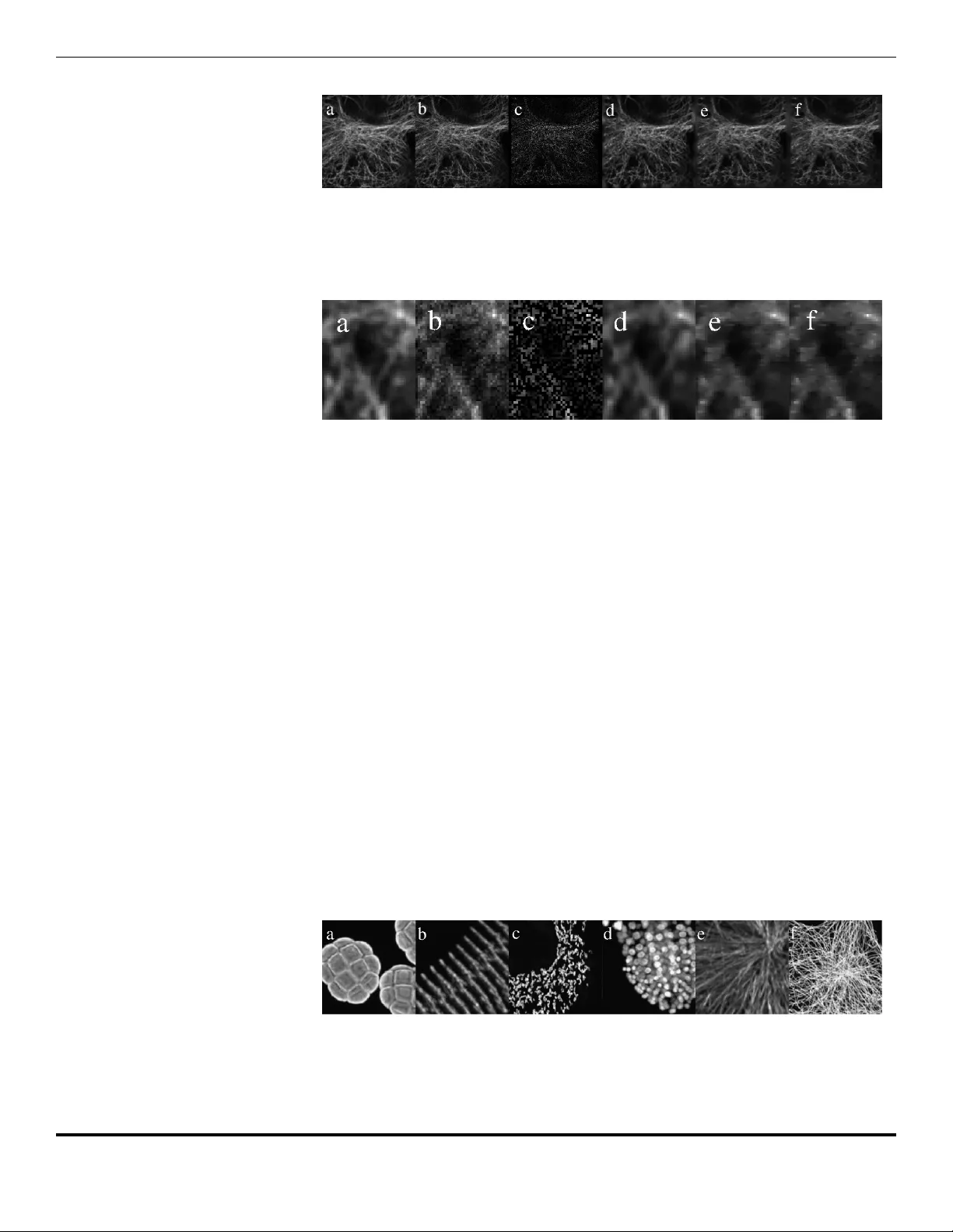
Image Reconstruction from Undersampled Confo cal Microscop y Data using Multiresolution Based Maxim um En trop y Regularization 1 Bibin F rancis 1 , Mano j Mathew 2 , Muth uvel Arigo vindan 1 , 1 Imaging Systems Lab, Electrical Engineering, Indian Institute of Science (I ISc), Bangalore, 560012, India 2Cen tral Imaging & Flow Cytometry F acilit y , National Cen ter for Biological Sciences (NCBS), Bangalore 560065, India Corresp onding author: m vel@iisc.ac.in Abstract W e consider the problem of reconstructing 2D images from randomly under-sampled confo cal microscop y samples. The well kno wn and widely celebrated total v ariation regularization, whic h is the ` 1 norm of deriv atives, turns out to b e unsuitable for this problem; it is unable to handle b oth noise and under-sampling together. This issue is link ed with the notion of phase transition phenomenon observ ed in c ompr essive sensing researc h, which is essentially the break-down of total v ariation metho ds, when sampling density gets low er than certain threshold. The severit y of this breakdown is determined by the so-called mutual inc oher enc e b etw een the deriv ativ e op erators and measuremen t op erator. In our problem, the mutual incoherence is low, and hence the total v ariation regularization giv es serious artifacts in the presence of noise even when the sampling density is not very low. There has b een very few attempts in developing regularization metho ds that p erform b etter than total v ariation regularization for this problem. W e develop a multi-resolution based regularization metho d that is adaptive to image structure. In our approach, the desired reconstruction is formulated as a series of coarse-to-fine multi-resolution reconstructions; for reconstruction at each lev el, the regularization is constructed to be adaptive to the image structure, where the information for adaption is obtained from the reconstruction obtained at coarser resolution lev el. This adaptation is achiev ed b y using maxim um entrop y principle, where the required adaptive regularization is determined as the maximizer of en trop y sub ject to the information extracted from the coarse reconstruction as constrain ts. W e also utilize the directionally adaptiv e second order deriv atives for constructing the regularization with directions guided by the given coarse reconstruction, which leads to an impro ved suppression of artifacts. W e demonstrate the sup eriorit y of the prop osed regularization metho d ov er existing ones using sev eral reconstruction examples. 1 In tro duction Confo cal microscopy is a wide-spread to ol among cellular biologists for studying func- tionalit y and physiology of living cells, and it has a theoretical resolution that is b etter than that of the wide-field microscopy . Its effective resolution b ecomes comparable to 1 Submitted to IOP JINST 1/20 widefield microscop y , or even inferior to that of wide-field microscop y in the case of the long term live cell imaging b ecause of the noise. How ev er, it is still preferred o ver widefield microscopy by many researchers for the p ossible reason that the raw images can b e interpreted directly without any decon v olution. This means that it can b e applied in 2D+t mo de for observing fast cellular phenomena [13, 27]. In this viewpoint, the frame rate in confocal microscopy is limited b ecause of the p oin t-wise scanning. Most of the confo cal microscop es take 0 . 1 − 1 seconds to generate a single 2D image [34]. Moreo ver, the point wise scanning coupled with the pinhole screen in confo cal microscop e significantly reduces the num ber photons impinging on the detector. As a result, the signal-to-noise ratio (SNR) of the reconstructed image is lo w. T o comp ensate for this, the excitation intensit y should b e raised which will lead to photo-bleac hing and photo-toxicit y . Photo-bleac hing is the process b y which the dy e com bines with the atmospheric oxygen and b ecomes non-fluorescent. In practical cases, photo-bleac hing is reduced by reducing the level of oxygen in the system. Photo-toxicit y is the pro cess by whic h dye reacts with the living cell and in turn destroying it. The only wa y to con trol the photo-toxicit y is to compromise on the resolution by either by reducing the excitation in tensity , or b y increasing the pinhole size; while the former approac h leads to loss of resolution by means of in creased noise, the latter leads to loss of resolution in the form of increased blurring. Considering the problem of longer acquisition time, we find that there has b een a significan t progresses such as the use of acoustic-optic deflector (AOD) [14, 29], and the dev elopment of Nipk ow disc [35]; ho w ever the point scanning alw ays limits the acquisition sp eed. Our goal is to develop a computational to ol that will allow trading-off resolution against acquisition time. T o achiev e this, we dev elop a metho d to reconstruct a full 2D images from randomly sub-sampled confo cal measurements. The domain of scientific computing that deals with this problem is called the scattered data appro ximation (SD A). Scattered data approximation methods are broadly classified as mesh-based metho ds [17], Krigging-based metho ds [28], distance-weigh ted metho ds [26], p olynomial approximation metho ds [10], and roughness minimizing metho ds [8, 22]. Roughness minimizing metho ds ha ve b etter robustness to noise and fluctuations in sampling density . So, we restrict our surv ey to the roughness minimizing metho ds. Giv en the list of scattered sample lo cations { x i } N s i =1 , and corresp onding sample v alues { f i } N s i =1 , roughness minimizing metho d addresses the reconstruction problem as the follo wing minimization problem, u ∗ = argmin u N s X i =1 ( u ( x i ) − f i ) 2 + λR ( u ) , (1) where R ( u ) is the roughness functional. As the sample lo cations { x i } N s i =1 can b e arbitrary , the mathematically correct wa y to handle the ab ov e minimization problem is to search for minimum with a suitable space of con tin uous functions (not a discrete image), as done by the thin plate spline metho ds. The landmark pap ers [8, 22] analytically solve the ab o ve minimization with some reasonable assumptions on the search space with the follo wing form is regularization functional: R ( u ) = Z Z "  ∂ 2 u ( x ) ∂ x 2  2 + 2  ∂ 2 u ( x ) ∂ xy  2 +  ∂ 2 u ( x ) ∂ y 2  2 # dxdy . (2) Solving the ab o ve mathematical minimization problem leads to the following form of the solution u ∗ as giv en b elo w: u ∗ ( x ) = N s X i =1 w i φ ( k x − x i k 2 ) + p ( x ) , (3) 2/20 where φ ( x ) is the thin-plate spline (TPS), and p ( x ) is a degree-one 2D polynomial. Although this metho d is mathematically elegant, it suffers from the follo wing problem: (i) the w eights hav e to b e computed b y solving a ill-conditioned, dense, large system of equations whic h breaks down numerically when the num ber of samples, N s b ecomes higher few thousands; (ii) after computing the w eigh ts, the required regular image is not directly av ailable, and it has to be computed from the equation (3), which is an exp ensiv e op eration. The first problem is somewhat addressed by Radial basis function metho d [3, 5], and is fully eliminated b y the partition of unity metho d [6] b y slightly compromising on the reconstruction quality . The subspace v ariational metho d [1, 23] eliminates both problems presen t in the TPS metho d; how ev er, it requires solving a linear system of equations of size that is equal to the num ber of pixels in the final reconstructed image, whic h ma y require a large amoun t of memory , and may require sp ecially built sparse solvers. T o eliminate the need for storing large matrices , we developed a discrete formulation in [12]. First, the sets { x i } N s i =1 and { f i } N s i =1 are transformed into a pair of regular grid images as follo ws: c ( y ) = X i ∈N y w i ( y ) , w i ( y ) = tanh ( k y − x i k ) k y − x i k (4) h ( y ) = h 0 ( y ) /c ( y ) , h 0 ( y ) = X i ∈N y w i ( y ) f i , (5) where N y is set of indices such that the corresp onding sample lo cations are within the unit area neigh b orho od around y . With this, the p ossible reconstruction methods that w e in tend to analyze can be collectiv ely written as follows: u ∗ = argmin u X y c ( y ) ( h ( y ) − u ( y )) 2 + λ X y 3 X i =1 (( d i ∗ u ) ( y )) 2 ! p/ 2 | {z } R p ( u ) , (6) where { d i , i = 1 , 2 , 3 } ’s are discrete filters implementing deriv ative op erators ∂ ∂ x∂ x , ∂ 2 ∂ y ∂ y , √ 2 ∂ ∂ x∂ y . The actual cost solved in [12] is with p = 2, where w e demonstrated that reconstruction obtained by minimizing the abov e cost with p = 2 repro duces the mathematically exact solution (equations (1) , and (2) ) with go o d accuracy . F urther, minimizing the ab o ve cost does not require storing large matrices and only requires iterations inv olving filtering and arra y multiplications only . The metho d presen ted in [30] is sp ecial case of our work presented in [12], where the sample lo cations X are restricted to in a subset of regular grid p oin ts. One dra wback in reconstructing the required image via solving (6) with p = 2 is that it p enalizes the square of the roughness at each pixel lo cations, whic h causes o ver-smoothing of sharp region of the image. This is clearly undesirable for image reconstruction in general, and fluorescence image reco v ery in particular. Fluorescent images are made of piecewise smo oth regions separated by sharp intensit y changes. In fluorescen t imaging, the part of the sp ecimen to b e imaged is injected with a dye. Up on the excitation of the sp ecimen with a high intensit y laser b eam, only the dyed region emit ligh t and hence they app ear bright compared to other regions in the image. As a result of this, the fluorescent images hav e sharp edges, and hence quadratic regularization is not suitable. In general image recov ery problems suc h as deblurring of full fluorescence images [25], reconstruction from F ourier samples measured using magnetic resonance [20], tomo- graphic reconstruction [36], it has b een prov en that solving (6) with p = 1—in which 3/20 case the regularization is called the ` 1 regularization—giv es reconstruction with higher sharpness and resolution. The main reason for this improv emen t is that minimizing the absolute v alue of deriv ativ es b y setting p = 1 is that it allo ws a few large v alues of deriv ative magnitudes, while the quadratic roughness functional forbids any large deriv ativ e magnitude. Hence the regularization with p = 1 allo ws sharp edges in the reconstruction. The difference in performance b et ween these forms of regularization functionals corresp onding to p = 1 and p = 2 is ev en more pronounced when the noise is high. F or p < 1, it has b een demonstrated that we get further improv ed p erformance o ver the quadratic regularization functional as well as the ` 1 regularization functional in inv erse problems such as deblurring [24], and tomographic reconstruction [21]. In- terestingly , there are no rep orted method that use other than p = 2 for the current problem, i.e., the problem of reconstructing scattered spatial p oin t measuremen ts. In reconstruction trials inv olving minimization of (6) with p = 1, w e observ ed spike-lik e artifacts that app ear to be a kind of remnan ts of sample density distribution. It w as also rep orted that the reconstructions obtained with p ∈ (0 , 1] were actually worse than the ones obtained with p = 2 in terms structural similarit y measures [11]. A related problem is observed in inv erse problems such as the reconstruction from F ourier samples,tomographic reconstruction, where the image reconstruction using the regularization with p = 1 breaks down leading to reconstruction quality that is significan tly inferior to the quality yielded b y quadratic case, i.e., the case with p = 2. This effect is referred in the literature as phase transitions [7]. The under-sampling factor at which the reconstruction breaks do wn is determined b y the so-called mutual incoherence [4] b etw een the op erator inv olved in measuremen t and deriv ativ e op erator used to construct the regularization. The actual definition of mutual incoherence is b ey ond the scop e of this pap er. Ho wev er, it is sufficient to note that, for the problem addressed in the pap er, i.e., the reconstruction from spatial p oint measurements, m utual incoherence is the low est. Hence the phase-transition threshold on the sample densit y is significan tly higher, and hence the o ccurrence of spik es mentioned ab o ve is justified. A nov el metho d, named as anisotropic interpolation metho d, for reconstructing images from sparse, spatial p oint measuremen t has b een developed in [2]. Here the reconstruction is achiev ed by means of a series of quadratic regularized reconstructions, where each quadratic regularization is constructed using first order deriv ativ es such that it is directionally adaptive b y making use of the information from the previous reconstruction in the series. How ev er, this metho d is based on first order deriv ativ es and hence is not suitable for fluorescence image, as the fluorescence images are comp osed of sharp structures. In [11], w e developed a new multi-resolution based regularization metho d using probabilistic formulation, where the required reconstruction is obtained b y solving a series of reconstructions at different resolution. F or the reconstruction at eac h resolution lev el, the regularization is constructed using a probabilistic view p oint such that it is adaptive to the lo cal image structure; the lo cal image information is obtained from the previous reconstruction in the series. W e named this metho d as the MSDA metho d, and w e demonstrated that MSD A outp erforms both l 1 metho d (solving (6) with p = 1) and anisotropic metho d of [2]. In this pap er, we develop a further significantly improv ed regularization metho d for image reconstruction from non-uniformly under-sampled spatial point measurements. The current formulation is b etter than the previous one [11] in the following w ays: (i) it is designed to b e adaptive to lo cal image structure based on maximum en tropy principle; (ii) it utilizes image Hessian to construct directionally adaptive regularization designed to further reduce the distortions. In the next section, we pro vide a more detailed ov erview of existing metho ds by introducing the for mulation of maximum a p osteriori estimation; this will serve for introducing the notions required for the developmen t of the proposed metho d. In section 3, we dev elop our Hessian based maxim um entropic regularization 4/20 that is constructed based on the giv en prior estimate of the required solution. W e also a in tro duce the ov erall cost function that will lead to the proposed reconstruction metho d. In Section 4, we describ e the m ultiresolution approach for eliminating the need for prior estimate. In Section 5, w e provide experimental v alidation of the prop osed method, where we demonstrate that the proposed metho d outp erforms existing methods with significan t reduction in the amount of artifacts. 2 Regularized Reconstruction as MAP Estimation W e will first describ e the standard MAP approach that corresp onds to the reconstruction problem given in the equation (6) , and then will describ e the modifications that will lead to the MSD A metho d. Let X denote the set of sample lo cations, i.e., let X = { x 1 , x 2 . . . x N s } , and let f = [ f 1 , f 2 , . . . , f N s ] T denote the vector containing samples measured from the locations contained in the set X . Let h and c b e the image pair represen ting the measurement transformed using the rules given in the equations (4) and (5) . Note that h pla ys the role of f and c pla ys the role of X . F or a candidate image, u , its probability of b eing the source of measurement, h , is known as the p osterior probabilit y , which can b e expressed using Ba y es rule as p ( u | h, c ) = p ( h | u, c ) p ( u, k ) p ( h, c ) , (7) where p ( h | u, c ) is the probability of obtaining the measurement image h giv en the candidate u and the sample density map c , p ( h, c ) is the probability of obtaining the measuremen t image h giv en sampling densit y map c , and p ( u, k ) is prior probability with v ariance parameter k . In MAP approach, one determines the required image as the minimizer of the negative logarithm of p ( u | h, c ). Denoting J ( u, h, c ) = − log p ( u | h, c ), w e write J ( u, h, c ) = [ − log p ( h | u, c ) − log p ( u, k )] , (8) where we hav e ignored the term p ( h, c ) since it is indep enden t of u . The form of prior probabilit y that will lead to the most known forms of regularization functionals can b e written as p ( u, k ) = Y y exp ( − 1 k ( E [ u ] ( y )) p/ 2 ) , (9) where E [ u ] ( y ) is some roughness image obtained from the candidate image u ( y ), typically in the form of sum of squares of deriv ativ e chosen order. Using the ab ov e form in the equation (8), giv es J ( u, h, c ) = D ( u, h, c ) + 1 k X y ( E [ u ] ( y )) p/ 2 , (10) where D ( u, h, c ) = − log p ( h | u, c ), whic h is usually called the data fitting term. Note that p ( h | u, c ) is only determined b y the random pro cess that generates the noise in the original measuremen t vector f . Noise across the different comp onents are clearly indep enden t; ho wev er, the noise across different pixels of h are indep enden t only if, for eac h y , the pixel v alue of h comes from only one of the comp onent of f . This will b e true if the measuremen t sample density is smaller than the reconstruction grid density , whic h is the case in the problem w e are addressing in this pap er. With this assumption, and with assumption that the noise is Gaussian, D ( u, h, c ) is written as D ( u, h, c ) = 1 σ 2 X y c ( y ) ( h ( y ) − u ( y )) 2 , (11) 5/20 where σ 2 is the noise v ariance. Although the noise in fluorescence imaging is not strictly Gaussian, the abov e form is used for data fitting, b ecause of its low computational complexit y . It is customary to allo cate higher computational complexity for the prior, p ( u, k ) b ecause the pay-off is more, and hence the ab o ve form for D ( u, h, c ) is frequently used. Substituting this form in (10) giv es J ( u, h, c ) = 1 σ 2 X y c ( y ) ( h ( y ) − u ( y )) 2 + 1 k X y ( E [ u ] ( y )) p/ 2 . (12) The ab ov e cost b ecomes iden tical upto a scale factor, to that of minimization given in (6) with the substitution E [ u ] ( y ) = P 3 i =1 (( d i ∗ u ) ( y )) 2 and λ = σ 2 k . Since both σ 2 and k are usually unkno wn, λ is typically considered as an user parameter. No w, we can see how the MAP formulation helps to explain the reason for getting spiky artifacts that app ear in the reconstruction obtained by minimizing (12) with p = 1. F rom (9) , it is clear that the reconstruction obtained as the minimizer of (12) is based on the assumption that the roughness v alue at each pixel lo cation is independent of neigh b oring pixel lo cation, which is ob viously wrong. Since b oth the op erators inv olv ed in the cost—the deriv ative operator in the regularization and the Dirac delta in the data fitting part—are lo calized, ignoring dep endency of the roughness at a pixel lo cation to that of its neighbors, causes the spikes to app ear in the reconstruction under the sparsifying effect of setting p = 1. This do es not o ccurs when p = 2, b ecause in this case, minimizing R p do es not force the deriv ativ es to b e sparse. This idea might hav e some in teresting connections with the idea of phase transitions [7] analyzed in compressiv e sensing theory . T o mitigate the effect this problem, w e prop osed the following mo dification to the prior probabilit y p ( u, k ). Supp ose v denotes the low er resolution estimate of the original image that generated the measuremen t. W e use this as a guide for determining correction to b e applied for comp ensating the error incurred by the pixel-wise indep enden t assumption of the image roughness. Then, w e replace p ( u, k ) with the following form of probability: p ( u, v , k ) = Y y exp  − 1 k  E [ v ] ( y )  − q  E [ u ] ( y )  r  (13) Clearly here, E [ v ] ( y ) gives the weigh ts for comp ensating for the error incurred by the pixel-wise indep endent assumption. As evident, the w eight is essentially the recipro cal of the total roughness in the low er resolution image v . This is justified b ecause, if the a verage roughness around a pixel y in lo w resolution estimate, v , is high, then the probabilit y that the roughness b eing high in the required image u ∗ at lo cation y will also b e higher. No w w e rewrite (8) using (13) with p ( u, k ) replaced by p ( u, v , k ), and with − log p ( h | u, c ) replaced D ( u, h, c ) to get the following expression: J msda ( u, v , h, c ) = 1 σ 2 X y c ( y ) ( h ( y ) − u ( y )) 2 1 k X y ( E [ u ] ( y )) − q ( E [ u ] ( y )) r | {z } R msda ( u,v ) (14) Next, note that v is itself an unknown b ecause it dep ends on the original image. W e used a m ulti-resolution metho d to resolve this dependency problem. T o describ e the m ulti- resolution approac h, let L [ j ] denote a 2 j -fold 2D in terp olation op erator such that L [ j ] u is an image whose size is 2 j larger than that u . Let J ( j ) msda ( u, v , h, c ) = J ( L [ j ] u, v , h, c ) b e the cost given in the equation (14) applied on u after interpolating by the factor 2 j . This means that, if N × N is the size of h and c , then u in J ( j ) msda ( u, v , h, c ) denotes an N 2 j × N 2 j v ariable. Let J ( j ) ( u, h, c ) denote the cost deriv ed from the cost of equation (12) by the 6/20 same w ay . Let s denote the n umber of levels for implementing the multi-resolution. In the multi-resolution approach, we obtain the initializing reconstruction by the following minimization: u ( s ) = argmin u J ( s ) ( u, h, c ) (15) Using u ( s ) as initialization, m ulti-resolution based reconstruction in v olves a series of minimizations for j = s − 1 , s − 2 , . . . , 0 as given b elo w: v = L [ j +1] u ( j +1) (16) u ( j ) = argmin u J ( j ) msda ( u, v , h, c ) (17) Note that for j = 0, the final minimization, u (0) = argmin u J (0) msda ( u, v , h, c ) gives the required final reconstruction. Note that, in the m ulti-resolution lo op, the result of previous reconstruction play the role of v , whic h is the guide to determine the comp ensating weigh t for the current reconstruction. W e demonstrated exp erimen tally in [11] that the MSDA metho d outp erforms the ` 1 metho d and anisotropic interpolation metho d of [2]. F urther, the results of MSDA was observed to hav e less artifacts. Although MSD A p erformed b etter than ` 1 metho d and anisotropic metho d, we still found some artifacts in the reconstructions, alb eit the amount of artifacts is significantly less. A p ossible discrepancy that could cause this artifact is that there is some lev el of arbitrariness in the comp ensation for the error incurred by pixel-wise indep endence assumption on the roughness. Sp ecifically , in the form of probability giv en in the (13) , E [ v ] ( y ) works as the av eraged v alue for E [ u ] ( y ) to b e used for the comp ensating w eight. This idea is actually put to work in the multiresolution lo op sp ecified by the equations (16) and (17) . F or reconstruction at scale i , w e minimize J ( i ) msda ( u, v , h, c ), con taining the regularization R msda ( L [ i ] u, v ) whic h is defined on L [ i ] u with comp ensating weigh ts extracted from v = L [ i +1] u ∗ ( i +1) . Clearly L [ i +1] u ∗ ( i +1) is some sort of a veraged version of the minimizer of J ( i ) msa ( u, v , h, c ), which is L [ i ] u ∗ ( i ) . How ev er, we do not hav e a direct relation betw een them, and hence the following question is left unansw ered: what is the optimal amount of av eraging required for defining the comp ensating weigh t? The a veraging is implicitly determined by the in terp olation filter used in the definition of L [ i ] ’s. This arbitrariness is probably the reason for the artifacts observed in the reconstruction of MSD A. 3 The prop osed metho d: Maxim um en tropic regular- ized reconstruction 3.1 Hessian and directional deriv ativ es Our construction of regularization was inspired from Hessian-Schatten norm introduced b y Lefkimmiatis et al. [19]. The Hessian op erator for con tinous function is given by ∇ 2 = " ∂ 2 ∂ x 2 ∂ 2 ∂ x∂ y ∂ 2 ∂ x∂ y ∂ 2 ∂ y 2 # . (18) The Hessian of a 2D function is useful for computing directional second deriv ativ es. Second deriv ative of a function g ( y ) at p oin t y along a direction d is defined as ∂ 2 ∂ α 2 g ( y + α d ) | α =0 , which, for brevit y we denote by ∂ dd . It can b e shown that ∂ dd g ( y ) = d T ∇ 2 g ( y ) d . F or any t wo linearly indep enden t direction vectors d 1 and d 2 , we can define mixed directional deriv ativ e as ∂ 2 ∂ α 1 ∂ α 2 g ( y + α 1 d 1 + α 2 d 2 ) | α 1 =0 ,α 2 =0 , which we denote 7/20 b y ∂ d 1 d 2 . It can b e shown that this becomes equal to ∂ d 1 d 2 g ( y ) = d T 1 ∇ 2 g ( y ) d 2 . The discrete equiv alen t of Hessian that can b e applied on discrete images can b e expressed as H ( y ) =  d xx ( y ) d xy ( y ) d xy ( y ) d y y ( y )  , (19) where d xx , d y y and d xy are discrete filters implementing the corresp onding deriv ativ es. W e use the same notations for the discrete directional deriv ativ es, and write ∂ dd g ( y ) = d T [( H ∗ g )( y )] d , and ∂ d 1 d 2 g ( y ) = d T 1 [( H ∗ g )( y )] d 2 . Here the notation ( H ∗ g )( y ) represen ts conv olving the matrix filter H with image g to get a 2 × 2 matrix of images, and then accessing the matrix corresp onding to the pixel lo cation y . The Hessian- Sc hatten norm is actually a family of norms and we present only a restricted, but most useful form b elo w: R hs ( g , p ) = X y k ( H ∗ g )( y ) k S ( p ) , (20) where k ( · ) k S ( p ) is Schatten norm of order p = [1 , ∞ ], which is essentially l p norm of the Eigen v alues of its matrix argument. The ab o ve cost can b e re-written as R hs ( g , p ) = X y [ |E 1 (( H ∗ g )( y )) | p + |E 2 (( H ∗ g )( y )) | p ] 1 /p (21) where E 1 ( · ) and E 2 ( · ) denote the op erators that return the Eigen v alues of the matrix argumen t. F rom the expression for directional deriv ativ e given ab ov e, and from the fact that the Eigen v ectors of a symmetric matrix are orthogonal, it can b e sho wn that E 1 (( H ∗ g )( y )) = ∂ ¯ g 1 ( y ) ¯ g 1 ( y ) g ( y ) = (22) ( ¯ g 1 ( y )) T [( H ∗ g )( y )] ¯ g 1 ( y ) , and E 2 (( H ∗ g )( y )) = ∂ ¯ g 2 ( y ) ¯ g 2 ( y ) g ( y ) = (23) ( ¯ g 2 ( y )) T [( H ∗ g )( y )] ¯ g 2 ( y ) , where ¯ g 1 ( y ) and ¯ g 2 ( y ) are the Eigen vectors of ( H ∗ g )( y ). In other words, the Eigen v alues of ( H ∗ g )( y ) are the directional deriv atives of g ( y ) taken along the Eigen directions of the Hessian. It can also b e shown that the cross deriv ativ e satisfy ∂ ¯ g 1 ( y ) ¯ g 2 ( y ) u ( y ) = ( ¯ g 1 ( y )) T [( H ∗ g )( y )] ¯ g 2 ( y ) = 0. 3.2 Maxim um entropic probability density on directional deriv a- tiv es The main goal here to is develop an improv ed form for the prior probability , p ( g , v , k ), where g is the underlying image that generated the measurement, and v is prior estimate of the required image, which we call the structure guide. The idea is to build this prior probabilit y on the distribution of Eigen v alues of the Hessian of g in a spatially adaptiv e manner, where the information for spatial adaptation is extracted from v . T o this end, w e define the directional deriv ativ es applied on image v with directions sp ecified b y the Eigen v ectors of the Hessian of g , as given b elo w: D 1 ,g ( v ( y )) = ∂ ¯ g 1 ( y ) ¯ g 1 ( y ) v ( y ) (24) = ( ¯ g 1 ( y )) T [( H ∗ v )( y )] ¯ g 1 ( y ) , D 2 ,g ( v ( y )) = ∂ ¯ g 2 ( y ) ¯ g 2 ( y ) v ( y ) (25) = ( ¯ g 2 ( y )) T [( H ∗ v )( y )] ¯ g 2 ( y ) , 8/20 With the ab o v e notation, we can observe that D 1 ,g ( g ( y )) = E 1 (( H ∗ g )( y )) , (26) D 2 ,g ( g ( y )) = E 2 (( H ∗ g )( y )) . (27) No w our goal can b e stated as to build prior probability mo del for the distribution of D 1 ,g (( g ( y )) and D 2 ,g (( g ( y )) based on the prior information present in D 1 ,g (( v ( y )) and D 2 ,g (( v ( y )). T o this end, we make the following hypotheses: • [H1] : F or each pixel location y , D i,g ( v ( y )) will b e a estimate of mean for D i,g ( g ( y )). This is justified, b ecause, the deriv ativ e op erators are linear op erators, v is smo othed v ersion of the required solution g . • [H2] : A larger v alue of |D i,g ( v ( y )) | indicates a smaller spatial supp ort of features con tributing to it. This means that—if D i,g ( v ( y )) is appro ximately related to D i,g ( g ( y )) by smo othing with a window—there is a larger uncertaint y on the exact lo cation of such features within this windows. Hence, provided that D i,g ( v ( y )) is an unbiased estimate of mean for D i,g ( g ( y )), |D i,g ( v ( y )) | will also b e prop ortional to the v ariance of D i,g ( g ( y )). Allowing an user parameter, q > 0, w e designate that this v ariance is k |D i,g ( v ( y )) | q , where k is a prop ortionalit y constant. • [H3] : The closeness of v to the required solution g determines the magnitude of k . Higher closeness will corresp onds low er magnitude of k . It should b e emphasized that the second h ypothesis do es not mean that the local v ariance of D i,g ( g ( y )) within a neighborho o d around y is given b y D i,g ( v ( y )). It actually means the follo wing: for any giv en v alue z , if { y j } M j =1 is the list of points suc h that D i,g ( v ( y j )) = z , j = 1 , . . . , M , then the v ariance of the sample set {D i,g ( g ( y j )) , j = 1 , . . . , M } is proportional to | z | q . Pro ving the v alidity of these h yp otheses is b eyond the scope this pap er. How ev er, the reconstruction result obtained by me ans of the regularization developed using these hypotheses will demonstrate the v alidit y implicitly . As we know the mean and v ariance of distribution of D i,g ( g ( y )), we use the maxi- m um entrop y principle for determine the prior probability , which says that, given the information derived from the data, the b est prior probability distribution that will lead to minimal distortion is the one that has the highest entrop y [15, 16]. F urther it is also kno wn that, if the v ariance and mean are kno wn, the probability mo del that has the highest entrop y is Gaussian mo del. Hence, the prop osed probability density function is giv en by p ( g , v , k ) = a Y y exp − 1 k 2 X i =1 ( D i,g ( g ( y )) − D i,g ( v ( y ))) 2 |D i,g ( v ( y )) | q ! , (28) where a is some normalization constant. Now the main problem in the ab o ve form of regularization functional is that, it is hard to minimize, as all the quantities inv olved are directional deriv atives, and directions are dep enden t on the unknown original image g . Hence, we prop ose the following mo difications. W e first, replace D i,g ( · ) by D i,v ( · ). This means essentially that, the directions for the directional deriv ativ es are now obtained from the prior estimate v . Hence we write the prior probability as given b elow: p ( g , v , k ) = a Y y exp − 1 k 2 X i =1 ( D i,v ( g ( y )) − D i,v ( v ( y ))) 2 |D i,v ( v ( y )) | q ! , (29) Here, D 1 ,v (( g ( y )) and D 2 ,v (( g ( y )) are similarly defined as defined in the equations (24) and (25) with the role of g and v in terchanged. In other words, these op erators are given 9/20 b y D 1 ,v ( g ( y )) = ∂ ¯ v 1 ( y ) ¯ v 1 ( y ) g ( y ) (30) = ( ¯ v 1 ( y )) T [( H ∗ g )( y )] ¯ v 1 ( y ) , D 2 ,v ( g ( y )) = ∂ ¯ v 2 ( y ) ¯ v 2 ( y ) g ( y ) (31) = ( ¯ v 2 ( y )) T [( H ∗ g )( y )] , ¯ v 2 ( y ) . where ¯ v 1 ( y ) and ¯ v 2 ( y ) are the Eigen v ectors ( H ∗ v )( y ) . As directions in the new op erators are indep enden t of the unknown image g , but obtained from the prior estimate v , the mo dified regularization functional given in the equation (29) is easy to minimize. Ho wev er, the modified cost p oses an another problem. W e observed that this mismatch in the directions lead to artifacts. This is p ossibly due to the fact that the correlation b et w een D 1 ,v (( g ( y )) and D 2 ,v (( g ( y )) is higher than the correlation betw een D 1 ,g (( g ( y )) and D 2 ,g (( g ( y )) due to the mismatc h in the directions. T o comp ensate for this, w e in tend to include the following op erator: D 1 , 2 ,v ( g ( y )) = ∂ ¯ v 1 ( y ) ¯ v 2 ( y ) g ( y ) = ( ¯ v 1 ( y )) T [( H ∗ g )( y )] ¯ v 2 ( y ) . (32) T o incorp orate D 1 , 2 ,v ( g ( y )) in the prior probabilit y , w e again need the estimated mean and v ariance. As done for D 1 ,v (( g ( y )) and D 2 ,v (( g ( y )), we can consider D 1 , 2 ,v ( v ( y )) to be the mean of D 1 , 2 ,v ( g ( y )). How ev er, the quantit y D 1 , 2 ,v ( v ( y )) is zero and hence it cannot serve for an estimate of v ariance of D 1 , 2 ,v (( g ( y )). W e prop ose use |D 1 ,v (( v ( y )) | q / 2 |D 2 ,v (( v ( y )) | q / 2 as the v ariance for D 1 , 2 ,v (( g ( y )). Hence the final form of prior probability can b e written as p me ( g , v , k ) = a Y y exp − 1 k 2 X i =1 ( D i,v ( g ( y )) − D i,v ( v ( y ))) 2 |D i,v ( v ( y )) | q (33) + ( D 1 , 2 ,v (( g ( y ))) 2 |D 1 ,v (( v ( y )) | q 2 |D 2 ,v (( v ( y )) | q 2  , In the ab ov e form, recall that D i,v ( g ( y )) is the directional second deriv ativ e applied on g along the direction given by the i th Eigen vector of Hessian of v at y . On the other hand, D i,v ( v ( y )) is the same directional op erator applied on v itself, which is actually the i th Eigen v alue of the Hessian of v at y . 3.3 The full cost for reconstruction By following the same conv en tion as that of the MSDA metho d, the negativ e log of p me ( · , v , k ) applied on the candidate image u (minimization v ariable) becomes the prop osed regularization, referred as the maxim um en tropic regularization. In other w ords, w e write, − log p me ( u, v , k ) = 1 k R me ( u, v ). Now the cost for the prop osed reconstruction metho d is obtained by replacing R msda ( u, v ) by R me ( u, v ) in the equation (14) , which is giv en b elo w: J me ( u, v , h, c ) = 1 σ 2 X y c ( y ) ( h ( y ) − u ( y )) 2 + 1 k R me ( u, v ) , (34) where R me ( u, v ) = X y " 2 X i =1 ( D i,v (( u ( y )) − D i,v (( v ( y ))) 2 |D i,v (( v ( y )) | q + (35) ( D 1 , 2 ,v (( u ( y ))) 2 |D 1 ,v (( v ( y )) | q / 2 |D 2 ,v (( v ( y )) | q / 2  10/20 F or notational con venience, we rewrite the ab o ve cost as given b elo w: J me ( u, v , h, c ) = X y c ( y ) ( h ( y ) − u ( y )) 2 + λR me ( u, v ) , (36) where λ = σ 2 k .As done is most image reconstruction methods, we will also impose a b ound constraint on the solution by mo difying the cost as giv en b elo w, ¯ J me ( u, v , h, v ) = J me ( u, v , h, c ) + X y B ( u ( y )) (37) where B ( u ( y )) is an indicator function for the range of allow able pixel v alues. B ( u ( y )) has a v alue of zero if 0 ≤ u ( y ) ≤ m and ∞ otherwise, where m is an user-sp ecified upp er b ound. The abov e cost can be minimized by a recently developed v ariant of ADMM metho d [9]. No w we recall that in MSDA, we had the question of optimal amount of smo othing that relates the structure guide and required image. The new metho d describ ed ab ov e is not based on this notion of comp ensation and hence this question is eliminated. Sp ecifically , in the new metho d prop osed here, if the prior estimate v is closer to the original image g , the prop ortionality constant, k is smaller as stated in the hypothesis [H3] . Hence, the clos eness of the minim um of ¯ J me ( u, v , h, v ), denoted by u ∗ , to the original image, g , is determined by the closeness of prior estimate to g . Also, b etter the closeness of v to original image, b etter will b e reconstruction. 4 F ractional multi-resolution based reconstruction 4.1 Multiresolution reconstruction The low resolution estimate, v is, of course, unkno wn as well. How ev er, w e can get around this problem by using a multiresolution approach as done in the developmen t of MSDA. Supp ose that we hav e a predefined decreasing sequence of integers { N i } s i =0 represen ting image sizes of a multiresolution pyramid where N 0 × N 0 is the size of c ( y ) and h ( y ). Let L i,j denote, with j > i , an upsampling op erator that interpolate an image of size N j × N j in to an image of size N i × N i . W e defer the description of the implemen tation of L i,j to later. In L i,j , we will hav e tw o p ossible v alues for i : either 0 or j + 1. L 0 ,j will b e used to define cost functions for level j . L j +1 ,j will b e used to generate initializations in the multi-resolution scheme as will b e explained later. With this, w e define the following cost function with upsampling: ¯ J ( j ) me ( u, v , c, h ) = X y c ( y ) ( h ( y ) − ( L 0 ,j u )( y )) 2 + (38) λR me ( L 0 ,j u, v ) + X y B (( L 0 ,j u )( y )) where ( L 0 ,j u )( y ) denotes accessing the pixel at y after upsampling of u from size N j × N j to size N 0 × N 0 . F urther, R me ( L 0 ,j u, v ), denotes applying R me ( u, v ) after upsampling u from size N j × N j to size N 0 × N 0 . W e will use the notational con ven tion that ¯ J (0) me ( u, v , c, h, λ ) = ¯ J me ( u, v , c, h, λ ). Note that, in ¯ J ( j ) me ( u, v , c, h ), size of the v ariable u is N j × N j . T o define the m ulti-resolution metho d, w e will also need the follo wing non-adaptiv e cost function for initializing reconstruction: J ( s ) ( u, c, h ) = X y c ( y ) ( h ( y ) − ( L 0 ,s u )( y )) 2 + λ X y 3 X i =1 (( d i ∗ ( L 0 ,s u )) ( y )) 2 ! (39) 11/20 Note that J ( s ) ( u, c, h ) in the ab o v e equation is essentially the quadratic cost given in the equation (6) except the difference that it is defined through the upsampling L 0 ,s . In the ab o v e equation, ( d i ∗ ( L 0 ,s u )) ( y ) denotes accessing pixel at lo cation y after applying con volution by d i on the upsampled image L 0 ,s u . With these definitions, we are ready to describ e m ultiresolution approac h. In the m ulti-resolution approach, we obtain the initializing reconstruction b y the following minimization: u ∗ ( s ) = argmin u J ( s ) ( u, c, h ) (40) Using u ∗ ( s ) as initialization, multi-resolution based reconstruction inv olves a series of minimizations for j = s − 1 , s − 2 , . . . , 0 as given b elo w: v = L 0 ,j +1 u ∗ ( j +1) (41) u ∗ ( j ) = argmin u ¯ J ( j ) me ( u, v , c, h ) (42) Note that for j = 0, the final minimization, u ∗ (0) = argmin u ¯ J (0) me ( u, v , h, c ) giv es the required final reconstruction. F rom the reconstruction represented by the equation (40), we observe the following: The initial reconstruction u ∗ ( s ) is obtained as an N s × N s arra y , which is of the smallest size in the pyramid. Here the regularization is not spatially adaptive, but, it is a standard quadratic regularization. How ever, since we are computing solution at coarsest resolution, this is acceptable. This result is only for initializing the multiresolution lo op. Next, from the multi-resolution loop represen ted b y the equations (41) and (42), we observ e that, at eac h step j , the reconstruction, u ∗ ( j ) is obtained b y minimizing the cost ¯ J ( j ) me ( u, v , c, h ) with resp ect to u . The ev aluation of the cost, ¯ J ( j ) me ( u, v , c, h ), on the minimization v ariable is actually carried out via upsampling by L 0 ,j from size N j × N j to size N 0 × N 0 . The structure guide for this cost is obtained from previous reconstruction, u ∗ ( j +1) , via upsampling by L 0 ,j +1 from size N j +1 × N j +1 to size N 0 × N 0 . As the lo op progresses, the structure guide improv es, which improv es the maximum entropic regularization, which in turn b ecomes the structure for the next reconstruction and so on. Clearly , at the end of the lo op, the reconstruction, u ∗ (0) will hav e less artifacts than the reconstruction obtained by standard ` 1 regularization, b ecause of this multiresolution based adaptive regularization. It should be noted that, at eac h step j , the minimization v ariable as well as the result of minimization, u ∗ ( j ) , is of size N j × N j . Note that the step sp ecified by the equation (42) itself requires iterative computation, which needs an initialization. An efficien t initialization can b e obtained from u ∗ ( j +1) b y upsampling op erator L j,j +1 , whic h generates an N j × N j image from an N j +1 × N j +1 . It should b e emphasized, in the definition of ¯ J ( j ) me ( u, v , c, h ), w e ha ve used the up- sampler L 0 ,j —whic h interpolates from size N j × N j to size N 0 × N 0 —for b oth the data fitting and regularization parts. Note that the interpolation is essential only for the data fitting part, and the regularizer can b e defined directly on the N j × N j image v ariable, u . How ev er, from our trials, we found that the current implementation pro duces b etter results. In a particular, the upsampled minima {L 0 ,j u ∗ ( j ) } s j =0 turn out to be b etter appro ximations to the original image g that generated the measured image h . This is imp ortan t because, at each step j , L 0 ,j +1 u ∗ ( j +1) w orks as the structure guide for obtaining the reconstruction u ∗ ( j ) . 4.2 F ractional multiresolution Note that the image size in most of the multiresolution sc hemes used so far in the literature satisfy N j N j +1 = 2. W e prop ose that, for better reconstruction results, this ratio 12/20 should b e a rational num ber in the op en interv al (1 , 2). W e will first justify the need for this, and then explain the sp ecific form of the sequence { N j } s j =0 and the implemen tation of the upsampling op erators {L i,j : 0 ≤ i, j ≤ s ; i < j } . W e first note that, in the sequence of minimization results in the m ulti-resolution, { u ∗ ( j ) } s j =0 , the reconstruction corresp onding to j = 0, u ∗ (0) is the final required recon- struction. The other reconstructions for j > 0 can b e considered to be the appro ximations to the final reconstruction; w e consider that the actual approximations are giv en b y the upsampled versions of these reconstructions, namely {L 0 ,j u ∗ ( j ) } s j =0 . Now, let g ∗ ( j ) denote the b est appro ximation for g , in sense of some matching criterion betw een L 0 ,j g ∗ ( j ) and g . No w, by applying argument given at the end of Section 3.3, we can say that the closeness of L 0 ,j u ∗ ( j ) to L 0 ,j g ∗ ( j ) is determined b y the closeness of the structure guide used in the reconstruction which is L 0 ,j +1 u ∗ ( j +1) . This in turn is determined b y how close is L 0 ,j +1 g ∗ ( j +1) to L 0 ,j g ∗ ( j ) . This suggests that the ratio N j N j +1 should b e sufficien tly low. How ev er, it should not b e to o low of course; otherwise s has b e a large n umber meaning that we will need to o man y steps in the multiresolution lo op. F or the conv enience of implementation, we consider the size to b e of the form N j = n s N d + ( s − j ) N d , for some p ositiv e integers n s and N d suc h that, for an y i and j in [0 , s ], the ratio N i N j will b e a rational num b er. Hence, the op erator L i,j with j > i , whic h denotes upsampling from size N j × N j to size N i × N i , is rational upsampling op erator. If N j N i = L j D i where L j and D i are some in teger with no common factors, then L i,j can b e implemented b y an L j -fold upsampling follow ed by a D i -fold downsampling. This can b e implemented using the following three steps [31, 32]:(i) expansion by a factor of L j along b oth axes which is essen tially inserting L j − 1 zeros for every sample along b oth axes; (ii) con v olv e with filter 1 L j (1 + z − 1 ) L j along b oth axes; (iii) decimation by a factor of D i whic h is discarding D i − 1 samples for ev ery blo c k of D i samples. 5 Exp erimen tal results Confo cal microscop e is a 3D imaging mo dality in which a series of p oint wise scanned 2D images are stack ed together. How ev er, it is often applied in 2 D + t mo de to observe fast cellular pro cesses. In this context, our goal is to suggest the prop osed metho d, which we name Maximum En tropic Regularized Reconstruction (MERR), as computationalto ol for optimally trading resolution against acquisition time, by acquiring p oint measurements only at randomly sub-sampled incomplete set of lo cations. W e also claim that our computational to ol allo ws to reduce photo-toxicit y because of its robustness against noise. T o demonstrate b oth claims, we generate tw o t yp e tes t data as given b elo w. • W e measure regular grid 2D images from a fixed sample, where one is acquired with full excitation in tensity , and others are acquired with different low er excitation in tensities. Different sample sets obtained by randomly selecting p oin ts from the low excitation images are used as test inputs for MERR, and the full 2D image corresp onding to highest exp osure intensit y is used as the ground truth for ev aluating the reconstruction quality . • W e select few 2D confo cal images from Nikon Small W orld rep ository as mo dels. F rom these mo dels, we sim ulate low excitation images b y adding mixed P oisson- Gaussian noise, and then generate randomly selected sample sets as inputs for reconstruction. The noiseless mo dels are used as ground truth for ev aluating the reconstruction qualit y . W e compare MERR with l 1 metho d [25], and MSDA metho d [11] in terms of structural similarit y (SSIM) [33] of the reconstructed image with resp ect to the ground truth. Note 13/20 that MERR is different from MSDA in t wo wa ys: (i) In MERR, the regularization is constructed using multiresolution based directionally adaptive filters by means of a maxim um entrop y formulation; on the other hands, in MSDA, the regularization is in an isotropic form with a m ultiresolution based reweigh ting; (ii) in MERR, we use fractional m ultiresolution, whereas in MSDA, standard multiresolution is used. W e do not compare with the ` 2 regularization here b ecause, we hav e already demonstrated the sup eriorit y of MSD A ov er ` 2 [11]. Since, the main goal here is to demonstrate the efficiency of maxim um en tropic regularization, we use the ground truth itself to tune the smo othing parameters for all the methods, and q for the prop osed metho d, MERR. While using the ground truth for tuning the smo othing parameter is common in the literature [18, 19], we need extra tuning effort for determining q . How ev er, in our exp eriments, the optimal v alue for q w as found indep endent of noise level and sample density , and was dep enden t only on the structure of the image. Hence, for a practitioner applying our metho d, the v alues of q can be kept fixed as long as the exp erimen t in volv es the same organelle. This situation is similar to that of MSDA, whose parameters q and r w ere dep enden t only on the nature of image structure [11]. F or determining optimal v alue for q , we p erformed grid search in the range 0 . 5 − 1 . 0 with step size 0 . 1. F or implementing |D i,v (( v ( y )) | q and |D i,v (( v ( y )) | q/ 2 , we used the appro ximations (  + |D i,v (( v ( y )) | ) q and (  + |D i,v (( v ( y )) | ) q/ 2 with  = 10 − 6 to ensure differentiabilit y . F or all reconstructions p erformed by MERR, w e set the parameters such that N d = 16 and N 0 / N s = 4 . While making N d smaller will alwa ys impro ve the reconstruction qualit y , the improv emen t w as found to b e insignifican t; on the other hand, the rise in the computational complexity b ecomes unaffordable. Similarly , in principle, making N 0 / N s larger can improv e the reconstruction quality , but, it did not significan tly improv e the reconstruction quality . 5.1 Exp erimen ts on real measured images F or our first exp erimen t, we imaged V ero cell lab eled with Abb erior Star 580 dye with imaging region of size of 52 . 2 µm × 51 . 2 µm comprising of 512 × 512 pixels. The images w ere taken with five levels of excitation intensities; the highest excitation intensit y was set suc h that the image is nearly noise-free, whic h will b e used as the ground truth. Other reduced intensit y levels w ere chosen to be 10% , 20% , 30%, and 40% of the highest. Figure 1.a shows the 256 × 256 cropp ed view of the image acquired at the full laser p ow er lev el and 1.b shows the cropp ed 256 × 256 image acquired at 40% laser p ow er level. F rom eac h of the images corresp onding to these four reduced levels of excitation, we extract fiv e sample set with densities 30% , 35% , 40% , 45%, and 50%. This makes a total of 20 test datasets. The reconstruction results from these 20 datasets are compared in table 1 and 2. F rom the tables, it is clear that the prop osed approac h, MERR, outp erforms b oth ` 1 and MSDA metho ds. Moreov er, it can b e observed that, for MERR, the optimal v alue of q remains constant indep enden t of noise level and the sample density , and is equal to 0 . 9. Moreo ver, the improv emen t yielded by MERR increases as the noise level increases. Among the compared metho ds, ` 1 metho d is the most sensitive one to noise yielding the lo west SSIM score. T o visually demonstrate the quality of reconstruction, we hav e provided the recon- struction results from 40% of samples taken from the image acquired at 40% laser p ow er in the figure 1. Figure 1.a shows the image obtained by imaging the V ero cell with full lase in tensity , which we designate as the ground truth image. Figure 1.b represents the image acquired at 40% laser p o wer level. F rom this 40% samples were drawn randomly to get the nonuniformly sampled image, which is sho wn in figure 1.c. Reconstructions obtained from this dataset using MERR, MSDA and ` 1 metho ds are given in the figures 1.d, 1.e, and 1.f resp ectiv ely . F rom the results, it is clear that the prop osed metho d yield b etter reconstruction than the existing ones. Moreov er, the prop osed metho d is b etter 14/20 Percen tage of laser power used Sampling Densities 30 35 40 MERR MSDA ` 1 MERR MSDA ` 1 MERR MSDA ` 1 40 0.792 0.771 0.737 0.811 0.788 0.760 0.826 0.800 0.772 30 0.783 0.759 0.727 0.794 0.770 0.742 0.807 0.780 0.753 20 0.753 0.731 0.697 0.771 0.745 0.716 0.779 0.754 0.726 10 0.714 0.682 0.657 0.730 0.706 0.679 0.742 0.717 0.689 T able 1. Comparison of SSIM score for ` 1 , MSDA, and MERR reconstructions for sampling densities from 30% to 40% of 256 × 256 images acquired at v arious laser p ow er lev els on the V ero Cell image (figure 1) Percen tage of laser power used Sampling Densities 45 50 MERR MSDA ` 1 MERR MSDA ` 1 40 0.831 0.805 0.779 0.837 0.812 0.790 30 0.814 0.784 0.763 0.822 0.800 0.774 20 0.788 0.762 0.735 0.800 0.774 0.749 10 0.749 0.722 0.695 0.755 0.731 0.708 T able 2. Comparison of SSIM score for ` 1 , MSDA, and MERR reconstructions for sampling densities from 45% to 50% of 256 × 256 images acquired at v arious laser p ow er lev els on the V ero Cell image (figure 1) suited to preserve the structures in the image whic h is resp onsible for the improv emen t in qualit y of reconstruction measured by the SSIM score. T o highlight this fact, we ha ve pro vided a zo omed in view of the reconstruction in the figure 2. F rom the figure, it is clear that ` 1 reconstruction has largest amount of artifacts in form of spikes. MSD A has reduced amount of artifacts, but the artifacts are still significant. On the other hand, there are no visible artifacts in the MERR reconstruction. It should be emphasized that there is a loss of resolution in reconstructed images of all three methods, whic h is inevitable because of noise and subsampling; ho w ever, the main factor that mak es MERR reconstruction sup erior is the absence of spiky artifacts. 5.2 Exp erimen ts on images with simulated noise The goal here is to compare MERR with other metho ds on images ha ving a v ariet y of structures. F or this purp ose, w e selected 6 images from Nikon Small W orld rep ository , whic h are display ed in the figure 3. W e hav e chosen the set such that the images hav e differen t types of distribution of deriv ative v alues. The T ublin image in 3.f is similar to the V ero cell image with identical structures and dense nonzero deriv ative co efficien ts. Ho wev er, the Golgi complex in 3.c has a sparse distribution of nonzero deriv ative v alues. All the remaining images in the figure hav e the deriv ativ e distribution in b et ween these t wo images. Hence, the selected set is a goo d representation for the biological images in the viewp oin t of testing the suitability of a new regularization scheme. These images are considered as the ground truth mo del, and to simulate measurements with v arying excitation intensities, we added v arying levels of noise. W e chose three lev els of noise suc h that the visual p erception of the noise lev el matc hes with noise level of images with 10% , 30% and 40% excitation intensities in the previous exp erimen ts. The corresp onding SNRs turn out to be 12 . 10 dB, 13 . 34 dB, and 14 . 34 dB resp ectiv ely . F rom each of these noisy images, we selected randomly selected sample sets with densities 30% , 40% and 50%. This makes a total of 6 × 3 × 3 = 54 test data sets. Reconstruction results of v arious metho ds applied on these set are compare in the table 3. F rom the table, it is clear that the relative p erformance of v arious metho ds are in the same order, and MERR outp erforms other metho ds. In figure 4, w e display images reconstructed from 40% of random samples from Thale cress ro ot image (Figure 3.d) with 14 . 34dB SNR. Here to o, it is clear that the prop osed approach clearly outp erforms the comp eting metho ds. A zo omed-in view of the comparison is given in the figure 5, where it is evident that the 15/20 Figure 1. a) Reference V ero Cell image acquired with full laser p ow er; b) V ero cell image acquired with 40% laser p o wer; c) Nonuniformly sampled V ero cell image obtained from (b) with 40% subsampling; d) Reconstruction obtained by MERR metho d from (c); e) Reconstruction obtained b y MSD A from (c); f) Reconstruction obtained b y ` 1 metho d from (c). Figure 2. Zo omed in view of figure 1 (physical size: 5 µm × 4 µm ) (a) Reference V ero Cell image acquired with full laser p ow er; b) V ero cell image acquired with 40% laser p o w er; c) Non uniformly sampled V ero cell image obtained from (b) with 40% subsampling; d) Reconstruction obtained by MERR metho d from (c); e) Reconstruction obtained b y MSDA from (c); f) Reconstruction obtained by ` 1 metho d from (c). reconstruction from MERR has least amount of artifacts, and ` 1 metho d has the highest amoun t of artifacts. 6 Conclusions W e addressed the problem of reconstructing 2D images from randomly undersampled noisy confo cal microscopy samples. While quadratic regularization functional that w ere originally used for this type of problems tend to o v er-smo oth the reconstructed images, total v ariation regularization functional—which is widely is used in solving in verse problems—results in artifacts in the reconstruction. W e developed a new type of regularization functional as negative logarithm of probability density function repre- sen ting the distribution of directional deriv ativ es of required image. The mo del for the probabilit y density function is inferred from a low er resolution estimate of required image based on the maximum entrop y principle. The problem of finding the low resolution estimate of the required image is systematically handled using a multiresolution approac h in volving a series of regularized reconstruction. W e demonstrated that the prop osed regularization metho d, named maximum entropic regularized reconstruction (MERR), yield significantly improv ed reconstruction compared to comp eting metho ds. Note that, Figure 3. T est images from Nikon Small W orld a) Acacia dealbata p ollen grains (Img1); b) Human cardiac my o cytes (Img2); c) Golgi complex (Img3); d) Thale cress ro ot (Img4); e) Epithelial cell in anaphase (Img5); f) T ubulin image (Img6). 16/20 Figure 4. Comparison of reconstruction results obtained from 40% of random samples from Thale cress ro ot image (Figure 3.d) with 14 . 34dB SNR. (a) ground truth; (b) noisy image with input SNR 14 . 34dB; (c) 40% of samples taken from (b); (d) reconstruction of MERR from (c); (e) reconstruction of MSDA from (c); (f) reconstruction of ` 1 metho d from (c). Figure 5. Zo omed-in view of figure 4 (ph ysical size: 5 . 1 µm × 5 . 1 µm ). (a) ground truth; (b) noisy image with input SNR 14 . 34dB; (c) 40% of samples taken from (b); (d) reconstruction of MERR from (c); (e) reconstruction of MSDA from (c); (f) reconstruction of ` 1 metho d from (c). in some case, the impro v emen t in SSIM score is as high as 0.07 which is very significant. Although we did not directly prov e the hypotheses used for building our maxim um en tropic probability mo del, the reconstruction results indirectly demonstrate the v alidit y the h yp otheses. References 1. M. Arigovindan, M. Suhling, P . Hunziker, and M. Unser. V ariational image reconstruction from arbitrarily spaced samples: A fast multiresolution spline solution. IEEE T r ansactions on Image Pr o c essing , 14(4):450–460, 2005. 2. A. Bourquard and M. Unser. Anisotropic interpolation of sparse generalized image samples. IEEE T r ansactions on Image Pr o c essing , 22(2):459–472, 2013. 3. M. D. Buhmann. R adial b asis functions: the ory and implementations , volume 12. Cam bridge universit y press, 2003. 4. E. Candes and J. Romberg. Sparsity and incoherence in compressive sampling. Inverse pr oblems , 23(3):969, 2007. 5. J. C. Carr, W. R. F right, and R. K. Beatson. Surface in terp olation with radial basis functions for medical imaging. IEEE tr ansactions on me dic al imaging , 16(1):96–107, 1997. 6. R. Ca voretto, A. De Rossi, and E. P erracc hione. P artition of unity interpolation on m ultiv ariate conv ex domains. International Journal of Mo deling, Simulation, and Scientific Computing , 6(04):1550034, 2015. 7. D. L. Donoho, A. Maleki, and A. Montanari. The noise-sensitivity phase transition in compresse d sensing. IEEE T r ansactions on Information The ory , 57(10):6920– 6941, 2011. 17/20 Images Input SNR (dB) Sampling Densities 30% 40% 50% MERR MSDA ` 1 MERR MSDA ` 1 MERR MSDA ` 1 Img1 14.34 0.871 0.839 0.799 0.884 0.857 0.821 0.898 0.871 0.842 13.34 0.861 0.832 0.790 0.875 0.845 0.807 0.884 0.856 0.807 12.10 0.838 0.811 0.770 0.862 0.818 0.784 0.873 0.834 0.816 Img2 14.34 0.934 0.903 0.884 0.937 0.907 0.888 0.941 0.913 0.894 13.34 0.926 0.895 0.871 0.933 0.902 0.879 0.933 0.903 0.880 12.10 0.912 0.869 0.841 0.916 0.879 0.851 0.920 0.895 0.869 Img3 14.34 0.902 0.870 0.840 0.918 0.895 0.870 0.924 0.906 0.890 13.34 0.885 0.853 0.810 0.891 0.871 0.862 0.911 0.889 0.883 12.10 0.861 0.842 0.800 0.886 0.859 0.833 0.898 0.860 0.858 Img4 14.34 0.888 0.857 0.834 0.902 0.873 0.857 0.909 0.885 0.857 13.34 0.879 0.847 0.842 0.896 0.868 0.845 0.899 0.865 0.851 12.10 0.866 0.826 0.803 0.879 0.845 0.823 0.889 0.854 0.843 Img5 14.34 0.853 0.831 0.763 0.871 0.822 0.807 0.885 0.837 0.817 13.34 0.841 0.811 0.750 0.855 0.845 0.794 0.884 0.856 0.807 12.10 0.838 0.804 0.740 0.842 0.818 0.784 0.873 0.834 0.792 Img6 14.34 0.798 0.725 0.682 0.834 0.764 0.727 0.854 0.791 0.761 13.34 0.783 0.706 0.661 0.819 0.745 0.707 0.838 0.772 0.742 12.10 0.746 0.676 0.632 0.792 0.715 0.676 0.819 0.750 0.718 T able 3. Comparison of SSIM scores for ` 1 , MSDA, and MERR metho ds from samples generated from the images giv en in the figure 3. 8. J. Duc hon. Splines minimizing rotation-inv ariant semi-norms in sob olev spaces. In Constructive the ory of functions of sever al variables , pages 85–100. Springer, 1977. 9. J. Eckstein and W. Y ao. Approximate admm algorithms derived from lagrangian splitting. Computational Optimization and Applic ations , 68(2):363–405, 2017. 10. M. F enn and G. Steidl. Robust lo cal approximation of scatterred data. In Ge ometric pr op erties for inc omplete data , pages 317–334. Springer, 2006. 11. B. F rancis, M. Mathew, and M. Arigovindan. Multiresolution-based weigh ted regu- larization for denoised image interpolation from scattered samples with application to confo cal microscopy . JOSA A , 35(10):1749–1759, 2018. 12. B. F rancis, S. Viswanath, and M. Arigovindan. Scattered data approximation by regular grid w eighted smo othing. Sadhana , 43(1):5, 2018. 13. S. Gonz´ alez and Z. T annous. Real-time, in viv o confo cal reflectance microscopy of basal cell carcinoma. Journal of the Americ an A c ademy of Dermatolo gy , 47(6):869– 874, 2002. 14. V. Iy er, B. E. Losa vio, and P . Saggau. Compensation of spatial and temporal disp ersion for acousto-optic multiphoton laser-scanning microscopy . Journal of biome dic al optics , 8(3):460–472, 2003. 15. E. T. Jaynes. Information theory and statistical mechanics. Physic al r eview , 106(4):620, 1957. 16. E. T. Jaynes. Information theory and statistical mec hanics. ii. Physic al r eview , 108(2):171, 1957. 17. M.-J. Lai. Scattered data interpolation and appro ximation using biv ariate c1 piecewise cubic p olynomials. Computer Aide d Ge ometric Design , 13(1):81–88, 1996. 18. S. Lefkimmiatis, A. Bourquard, and M. Unser. Hessian-based norm regularization for image restoration with biomedical applications. IEEE T r ansactions on Image Pr o c essing , 21(3):983–995, 2012. 18/20 19. S. Lefkimmiatis, J. P . W ard, and M. Unser. Hessian sc hatten-norm regularization for linear inv erse problems. IEEE tr ansactions on image pr o c essing , 22(5):1873– 1888, 2013. 20. M. Lustig, D. Donoho, and J. M. P auly . Sparse mri: The application of com- pressed sensing for rapid mr imaging. Magnetic R esonanc e in Me dicine: An Official Journal of the International So ciety for Magnetic R esonanc e in Me dicine , 58(6):1182–1195, 2007. 21. C. Miao and H. Y u. Alternating iteration for ` p (0 < p ≤ 1) regularized ct reconstruction. IEEE A c c ess , 4:4355–4363, 2016. 22. C. A. Micc helli. Interpolation of scattered data: distance matrices and conditionally p ositiv e definite functions. In Appr oximation theory and spline functions , pages 143–145. Springer, 1984. 23. O. V. Morozov, M. Unser, and P . Hunzik er. Reconstruction of large, irregularly sampled multidimensional images. a tensor-based approach. IEEE tr ansactions on me dic al imaging , 30(2):366–374, 2011. 24. M. Nikolo v a, M. K. Ng, and C.-P . T am. F ast nonconv ex nonsmo oth minimization metho ds for image restoration and reconstruction. IEEE T r ansactions on Image Pr o c essing , 19(12):3073–3088, 2010. 25. O. Scherzer. Denoising with higher order deriv ativ es of b ounded v ariation and an application to parameter estimation. Computing , 60(1):1–27, 1998. 26. D. Shepard. A tw o-dimensional interpolation function for irregularly-spaced data. In Pr o c e e dings of the 1968 23r d A CM national c onfer enc e , pages 517–524. ACM, 1968. 27. K. Sok olo v, M. F ollen, J. Aaron, I. P a vlo v a, A. Malpica, R. Lotan , and R. Ric hards- Kortum. Real-time vital optical imaging of precancer using an ti-epidermal growth factor receptor an tib o dies conjugated to gold nanoparticles. Canc er r ese ar ch , 63(9):1999–2004, 2003. 28. M. L. Stein. Interp olation of sp atial data: some the ory for kriging . Springer Science & Business Media, 2012. 29. R. Y. Tsien and B. J. Bacsk ai. Video-rate confo cal microscopy . In Handb o ok of biolo gic al c onfo c al micr osc opy , pages 459–478. Springer, 1995. 30. M. Unser. Multigrid adaptiv e image pro cessing. In Pr o c. IEEE Conf. Image Pr o c essing (ICIP’95) , volume 1, pages 49–52. IEEE, 1995. 31. M. Unser, A. Aldroubi, and M. Eden. B-spline signal pro cessing. ii. efficiency design and applications. IEEE tr ansactions on signal pr o c essing , 41(2):834–848, 1993. 32. M. Unser, A. Aldroubi, M. Eden, et al. B-spline signal pro cessing: Part i theory . IEEE tr ansactions on signal pr o c essing , 41(2):821–833, 1993. 33. Z. W ang, A. C. Bo vik, H. R. Sheikh, and E. P . Simoncelli. Image quality assessment: from error visibilit y to structural similarit y . IEEE tr ansactions on image pr o c essing , 13(4):600–612, 2004. 34. G. E. Wnek and G. L. Bo wlin. Confo cal microscop y/denis sem wogerere, eric r. weeks. In Encyclop e dia of Biomaterials and Biome dic al Engine ering , pages 737–746. CR C Press, 2008. 19/20 35. G. Xiao, T. R. Corle, and G. Kino. Real-time confocal scanning optical microscop e. Applie d physics letters , 53(8):716–718, 1988. 36. X. Zheng, I. Y. Chun, Z. Li, Y. Long, and J. A. F essler. Sparse-view x-ray ct recon- struction using ` 1 prior with learned transform. arXiv pr eprint arXiv:1711.00905 , 2017. 20/20