Coupled dictionary learning for unsupervised change detection between multi-sensor remote sensing images

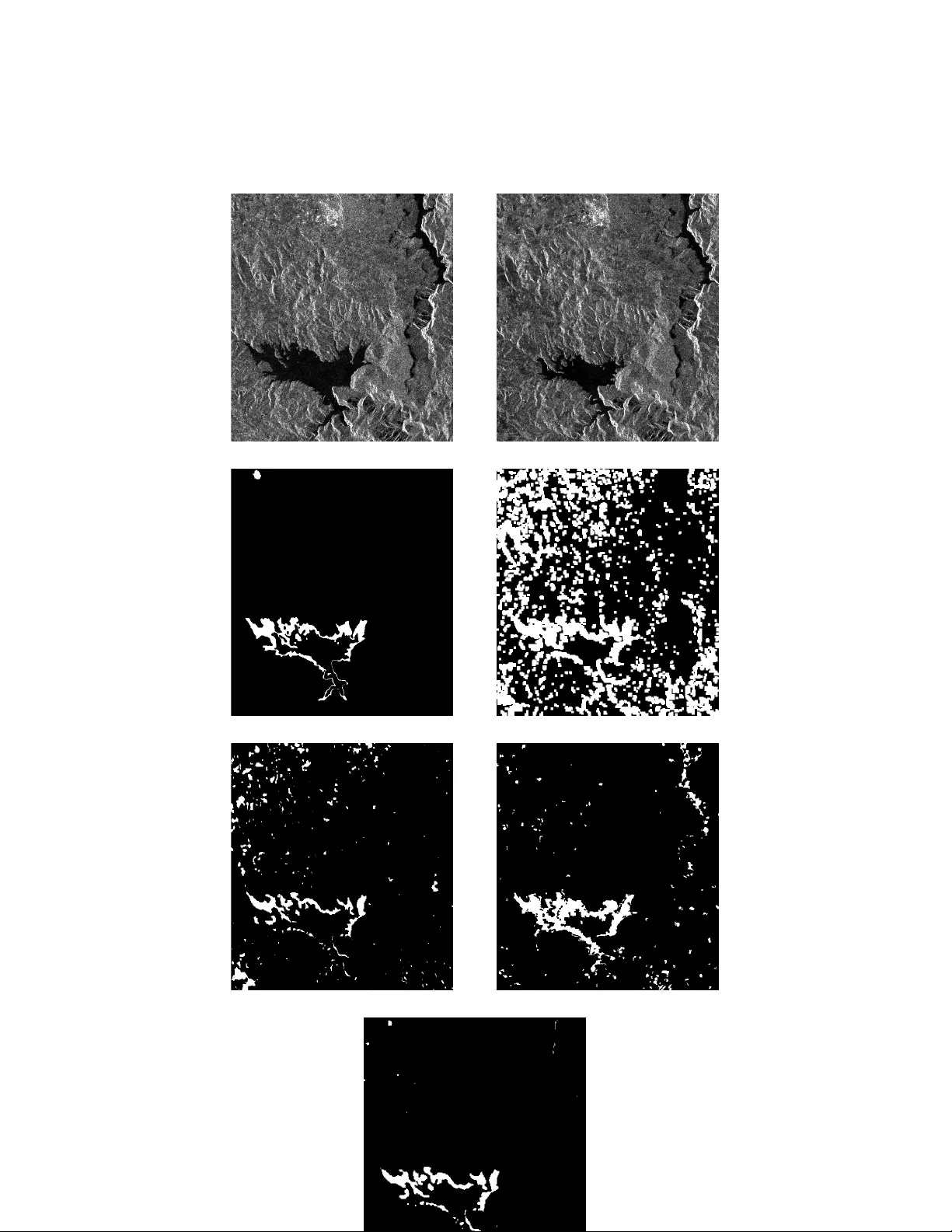
Coupled dictionary learning for unsupervised change detection between multi-sensor remote sensing images I V inicius Ferraris a, , Nicolas Dobigeon a , Y anna Cav alcanti a , Thomas Oberlin a , Marie Chabert a a University of T oulouse, IRIT/INP-ENSEEEIHT , 2 Rue Camichel, 31071 T oulouse, F rance Abstract Archetypal scenarios for change detection generally consider two images acquired through sensors of the same modality . Howe ver , in some specific cases such as emer- gency situations, the only images av ailable may be those acquired through sensors of different modalities. This paper addresses the problem of unsupervisedly detecting changes between two observed images acquired by sensors of dif ferent modalities with possibly different resolutions. These sensor dissimilarities introduce additional issues in the conte xt of operational change detection that are not addressed by most of the classical methods. This paper introduces a novel framew ork to effecti vely exploit the av ailable information by modelling the two observed images as a sparse linear combi- nation of atoms belonging to a pair of coupled overcomplete dictionaries learnt from each observed image. As they co ver the same geographical location, codes are expected to be globally similar , e xcept for possible changes in sparse spatial locations. Thus, the change detection task is en visioned through a dual code estimation which enforces spa- tial sparsity in the difference between the estimated codes associated with each image. This problem is formulated as an in verse problem which is iterativ ely solved using an efficient proximal alternating minimization algorithm accounting for nonsmooth and noncon vex functions. The proposed method is applied to real images with simulated I Part of this work has been supported by Coordenao de Aperfeioamento de Ensino Superior (CAPES), Brazil, the EU FP7 through the ERANETMED JC-W A TER program [MapIn vPlnt Project ANR-15-NMED- 0002-02] and the ANR-3IA Artificial and Natural Intelligence T oulouse Institute (ANITI). Email addr ess: firstname.lastname@enseeiht.fr (V inicius Ferraris) Pr eprint submitted to ELSEVIER journal September 4, 2019 yet realistic and real changes. A comparison with state-of-the-art change detection methods evidences the accurac y of the proposed strategy . 1. Intr oduction Ecosystems exhibit permanent variations at dif ferent temporal and spatial scales caused by natural, anthropogenic, or even both factors [ 16 ]. Monitoring spatial varia- tions ov er a period of time is an important source of knowledge that helps understand- ing the possible transformations occurring on Earth’ s surf ace. Therefore, due to the importance of quantifying these transformations, change detection (CD) has been an ubiquitous issue addressed in the remote sensing and geoscience literature [ 35 ]. Remote sensing CD methods can be first classified with respect to (w .r .t.) their supervision [ 6 ], depending on the a vailability of prior kno wledge about the e xpected changes. More precisely , supervised CD methods require ground reference information about at least one of the observations. Conv ersely , unsupervised CD can be conte xtual- ized as automatic detection of changes without the need for any further e xternal knowl- edge. Each class of CD methods present particular competitiv e advantages w .r .t. the others. For instance, supervised CD methods generally achieve better accurac y for pre- defined modalities whereas unsupervised methods are characterised by their flexibility and genericity . Nev ertheless, implementing supervised methods require the acquisi- tion of rele vant ground information, which is a v ery challenging and expensi ve task, in terms of human and time resources [ 6 ]. Relaxing this constraints makes unsupervised methods more suitable for operational CD. CD methods can also be categorized w .r .t. the imagery modalities the method is able to handle. As remote sensing encompasses man y dif ferent types of imagery modalities (e.g., single- and multi-band optical images, radar , LiDAR), dedicated CD methods hav e been specifically dev eloped for each one by exploiting its acquisition process and the intrinsic characteristics of the resulting data. Thus, due to dif ferences in the physical meaning and statistical properties of images from dif ferent sensor modali- ties, a general CD method able to handle all modalities is particularly difficult to design and to implement. For this reason, most of the CD methods focus on a pair of im- 2 ages from one single target modality . In this case, the images are generally compared pixel-wisely using the underlying assumption of same spatial resolutions [ 46 , 7 ]. Nev- ertheless, in some practical scenarios such as, e.g., emergency missions due to natural disasters, when the a v ailability of data and the responsiv eness are strong constraints, CD methods may hav e to handle observations of dif ferent modalities and/or resolu- tions. This highlights the need for robust and flexible CD techniques able to deal with this kind of observations. The literature about multimodal CD is very limited, yet a few rele v ant references in- clude the works by Kawamura [ 34 ], Bruzzone et al. [ 9 ], Inglada [ 32 ], Lu et al. [ 35 ], Al- berga et al. [ 2 ], Mercier et al. [ 41 ] and Prendes et al. [ 44 ]. Howe ver , multimodal CD has always been an important topic since the initial dev elopment of CD methods. Earlier work by Kawamura [ 34 ] described the potential of CD between a multimodal collec- tion of datasets (e.g., photographic, infrared and radar), applied to weather prediction and land surv eillance. Three features are e xtracted from the pair and the CD algorithm is trained on a learning set. According to Lu et al. [ 35 ], various methods dedicated to CD between images from different sources of data are grouped as geographical infor- mation system-based methods. For instance, Solberg et al. [ 48 ] proposed a supervised classification of multisource satellite images using Markov random fields. The work of Bruzzone et al. [ 9 ] uses compound classification to detect changes in multisource data. The method uses artificial neural networks to estimate the posterior probability of classes. Moreo ver , Inglada [ 32 ] studies the relev ance of several similarity measures between multisensor data. These measures are implemented in a CD conte xt [ 2 ]. A preprocessing technique based on conditional copula that contrib utes to better statis- tically modeling multisensor images was proposed by Mercier et al. [ 41 ]. Besides, Brunner et al. [ 8 ] presented a strategy to assess building damages using a pair of very high resolution (VHR) optical and radar images by geometrically modeling buildings in both modalities. Chabert et al. [ 12 ] updated information databases by means of lo- gistic regression. More recently , the work of Prendes et al. [ 44 ] presented a supervised method to infer changes after learning a manifold defined by pairs of patches extracted from the two images. Although some of these methods present relativ ely high detec- tion performance, they are often restrained to a specific modality or to a specific target 3 application. For instance, Solano-Correa et al. [ 47 ] proposed an approach to detect changes between multispectral images with different spatial and spectral resolutions by homogenization of radiometric and geometric image properties. Ho wev er, this ap- proach relies in particular on a taxonomy of possible radiometric changes observed in very high resolution images. Moreover , some methods are only suitable for build- ing damage assessment taking benefit of their high-lev el modeling, b ut sho w a poor adaptability to other scenarios [ 8 , 12 ]. The other ones estimate some metrics from un- changed trained samples, which prevents their application within a fully unsupervised context [ 9 , 44 , 41 ]. Recently , an unsupervised multi-source CD method based on coupled dictionary learning was addressed by Gong et al. [ 30 ]. In the proposed methodology , the CD is based on the reconstruction error of patches approximated thanks to estimated coupled dictionary and independent sparse codes. Atoms of the dictionary are learnt from pairs of patches jointly extracted from the observed images. F ollowing the same principle, in Lu et al. [ 36 ], a semi-supervised method was used to handle multispectral images based on joint dictionary learning. Both methods rely on the rationale that the coupled dictionary estimated from the observed images tends to produce stronger reconstruction errors in change regions rather than in unchanged ones. Because of the multi-modality , the problem has not been formulated in the image space, but rather in a latent space formed by the coupled dictionary atoms. Ho wever , both methods exhibit some crucial issues that may impair their relativ e performance. First, the underlying optimization problem is highly noncon vex and no con vergence guarantees are ensured, ev en by using some traditional dictionary learning methods [ 1 ]. Then, the considered CD problem has been split into two distinct steps: dictionary learning and code estimation. The errors in code estimation may produce false alarms in the final CD e ven with reliable dictionary estimates. Also, the statistical model of the noise – inherent to each sensor modality – has not been taken into consideration explicitly , which may dramatically impact the CD performance [ 10 ]. Finally , these methods do not consider overlapping patches, which potentially would increase their rob ustness and thus do not explicitly handle the problem of possible dif ferences in spatial resolutions [ 24 , 23 ]. The adequacy between the size of patches and the image scale is not discussed, although it may have a negati ve 4 impact on the dictionary coupling and thus on the detection performance. Overcoming these limitations, this paper proposes a similar methodology to learn coupled dictionaries able to con veniently model multimodal remote sensing images. Specifically , contrary to the aforementioned methods, the problem is fully formulated without splitting the learning and coding steps. Also, an appropriate statistical model is deriv ed to describe the image from each specific remote sensing modality . Besides, the proposed method explicitly allows patch o verlapping within the overall estimation pro- cess. T o couple images with different resolutions, additional scaling matrices inspired by the work by Seichepine et al. [ 45 ] are jointly estimated within the whole process. Fi- nally , as the problem is highly noncon ve x, it is iterati vely solved based on the proximal alternating linearized minimization (P ALM) algorithm [ 5 ], which ensures con vergence tow ards a critical point for some nonconv ex nonsmooth problems. Note that the pro- posed patch-based method departs from segmentation-based methods which generally extract change information at an object-le vel, whose resolution is implicitly defined by the chosen segmentation procedure [ 22 ]. Instead, the proposed method linearly de- composes o verlapping square patches onto an appropriate common latent space, which allows CD to be operated at a pix el level. This manuscript is organized as follows. Generic and well-admitted image models are introduced in Section 2 . Capitalizing on these image models, Section 3 formulated the CD problem as a coupled dictionary learning. Section 4 proposes an algorithmic solution to minimize the resulting CD-based objectiv e function. Section 5 reports ex- perimental results obtained on synthetic images, considering three distinct simulation scenarios. Experiments conducted on real images are presented in Section 5.3 . Finally , Section 6 concludes the manuscript. 2. Image models 2.1. F orwar d model Let us consider that the image formation process inherent to all digital remote sens- ing imagery modalities is modeled as a sequence of transformations, denoted T [ · ] . This sequence applies to the original scene to produce the sensor output image. This output 5 image is referred to as the observ ed image and is denoted by Y ∈ R L × N consisting of N voxels y i ∈ R L stacked lexicographically that is from left to right, row by row . The voxel dimension L may represent different quantities depending on the modality of the data. F or instance, it stands for the number of spectral bands in the case of multiband optical images [ 24 ] or for the number of polarization modes in the case of polarimetric synthetic aperture radar (POLSAR) images. The observ ed image provides a limited representation of the original scene with properties imposed by the image signal processor characterizing the sensor . The original scene cannot be exactly repre- sented because of its continuous nature, but it can be con veniently approximated by a latent (i.e., unobserved) image X ∈ R L × N related to the observed image as follo ws Y = T [ X ] . (1) The sequence of transformations T [ · ] operated by the sensor over the latent image is often referred to as the de gradation pr ocess . It may represent resolution degradations accounting for the spatial and/or spectral characteristics of the sensor [ 23 , 24 ]. In this paper, it specifically models the intrinsic noise corruption associated to the sensor modality [ 50 ]. The latent image X can be understood, in this context, as a noise-free version of the observ ed image Y with the same resolution. More precisely , the transformation T [ · ] underlies the likelihood function p ( Y | X ) which statistically models the observed image Y conditionally to the latent image X by taking into account the noise statistics. The noise statistical model mainly depends on the modality and rely on some classical distributions, e.g., the Gaussian distribution for optical images or the Gamma distribution for multi-look SAR images. Moreover , as already pointed out by F ´ evotte et al. [ 25 ] in a different application context, for a wide family of distributions, this likelihood function relies on a diver gence measure D ( ·|· ) between the observed and latent images, which finally defines an explicit data-fitting term through a negati ve-log transformation − log p ( Y | X ) = φ − 1 D ( Y | X ) + θ (2) 6 where φ and θ are parameters characterizing the distributions. In Appendix A , the div ergence measures D ( ·|· ) are deri ved for two of the most common remote sensing image modalities, namely optical multiband and SAR images, considered in this work. 2.2. Latent imag e sparse model Sparse representations hav e been an ubiquitous and well-admitted tool to model images in v arious applications and task-driven contexts [ 38 ]. Indeed, natural im- ages are known to be compressible in a transformed domain, i.e., they can be ef- ficiently represented by a fe w expansion coefficients acting on basis functions [ 40 ]. This finding has motiv ated numerous works on image understanding, compression and denoising [ 42 , 14 ]. In earlier works, this transformed domain, equi v alently de- fined by the associated basis functions, was generally fixed in advance and chosen in agreement with the expected spatial content of the images [ 40 ]. Thus, the basis func- tions belonged to pre-determined families with specific representation abilities, such as cosines, wav elets, contourlets, shearlets, among others. More recently , the seminal contribution by Aharon et al. proposed a new paradigm by learning an overcomplete dictionary jointly with a sparse code [ 1 ]. This dictionary learning-based approach ex- ploits the key property of self-similarity characterizing the images to provide an adap- tiv e representation. Indeed, it aims at identifying elementary patches that can be lin- early and sparsely combined to approximate the observ ed image patches. In this paper , following the approach by Aharon et al. [ 1 ], we propose to resort to this dictionary- based representation to model the latent image X . More precisely , the image is first decomposed into a set of N p 3D-patches with 1 ≤ N p ≤ N . Let R i : R L × N → R K 2 L denote a binary operation modeling the e xtraction, from the image, of the i th patch ( i ∈ { 1 , . . . , N p } ) such that p i = R i X (3) where p i ∈ R K 2 L stands for the i th K × K × L -pixel patch in its v ectorized form. The integer K > 1 defines the spatial size of the patches, i.e., its number of rows and columns before being vectorized. Note that the number of patches N p is such that 1 ≤ N p ≤ N and patches may overlap. The choice of the number N p of patches will 7 be more deeply discussed in Section 3 in the specific context of CD. The conjugate of the patch-extraction operator 1 , denoted R T i , acts on p i to produce a zero-padded image composed by the unique patch p i located at the i th spatial position. In accordance with dictionary-based representation principles, these patches are assumed to be approximately and independently modeled as sparse combinations of atoms belonging to an ov ercomplete dictionary D = [ d 1 , · · · , d N d ] ∈ R K 2 L × N d p i | D , a i ∼ N  Da i , σ 2 I N d  (4) where N d > 0 stands for the user-defined number of atoms composing the dictionary , commonly referred to as dictionary size and a i ∈ R N d represents the code (coeffi- cients) of the current patch over the dictionary , Σ = σ 2 I N d is the error cov ariance matrix and . Let P ∈ R K 2 L × N p =  p 1 , · · · , p N p  denote the matrix that stacks the set of all, possibly overlapping, patches extracted from the latent image X at N p spatial positions arranged on a generally regular spatial grid and enumerated in a lexi- cographical order (i.e., from left to right and top to bottom of the image). The matrix A ∈ R N d × N p =  a 1 , · · · , a N p  is the code matrix in which each column represents the code for each corresponding column of P . The o vercompletness property of the dictionary , occurring when the number of atoms is greater than the effecti ve dimen- sionality of the input space, N d  K 2 L , allows for the sparsity of the representation [ 42 ]. The overcompletness implies redundancy and non-orthogonality between atoms. This property is not necessary for the decomposition, b ut has been proved to be very useful in some applications like denoising and compression [ 1 ]. Giv en the image patch matrix P , dictionary learning aims at reco vering the set of atoms D and the associated code matrix A and it is generally tackled through a 2-step procedure. First, inferring the code matrix A associated with the patch matrix P and the dictionary D can be formulated as a set of N p sparsity-penalized optimization problems. Sparsity of the code vectors a i = [ a 1 i , . . . , a N d i ] T ( i = 1 , . . . , N p ) can be promoted by minimizing 1 Note that, despite a slight abuse of notation, the operator R (resp., R T ) does not stand for a matrix, but rather for a linear operator acting on the image X (resp., the patch p i ) directly . 8 its ` 0 -norm. Howe ver , since this leads to a non-conv ex problem [ 14 ], it is generally substituted by the corresponding con vex relaxation, i.e., an ` 1 -norm. Within a proba- bilistic frame work, taking into account the e xpected non-negativ eness of the code, this choice can be formulated by assigning a single-side exponential (i.e., Laplacian) prior distribution to the code components, assumed to be a priori independent a i ∼ N d Y j =1 L ( a j i ; λ ) (5) where λ is the hyperparameter adjusting the sparsity lev el over the code. Con versely , learning the dictionary D giv en the code A can also be formulated as an optimization problem. As the number of solutions for the dictionary learning problem can be ex- tremely large, one common assumption is to constrain the energy of each atom, thereby prev enting D to become arbitrarily large [ 39 ]. Moreo ver , in the particular conte xt con- sidered in this work, to promote the positivity of the reconstructed patches, the atoms are also constrained to positiv e values. Thus, each atom will be constrained to the set S , n D ∈ R K 2 L × N d + | ∀ j ∈ { 1 , . . . , N d , } k d j k 2 2 = 1 o . (6) 2.3. Optimization pr oblem Adopting a Bayesian probabilistic formulation of the image model introduced in Sections 2.1 and 2.2 , the posterior probability of the unknown variables X , D and A can be deriv ed using the probability chain rule [ 29 ] p ( X , D , A | Y ) ∝ p ( Y | X ) p ( X | D , A ) p ( D ) p ( A ) (7) where p ( Y | X ) is the likelihood function relating the observation data to the latent image through the direct model ( 1 ), p ( X | D , A ) is the dictionary-based prior model of the latent image, p ( D ) and p ( A ) are the (hyper -)prior distributions associated with the dictionary and the sparse code. Under a maximum a posteriori (MAP) paradigm, the joint MAP estimator n ˆ X MAP , ˆ D MAP , ˆ A MAP o can be deri ved by minimizing the 9 negati ve log-posterior , leading to the following minimization problem n ˆ X MAP , ˆ D MAP , ˆ A MAP o ∈ argmin X , D , A J ( X , D , A ) (8) with J ( X , D , A ) = D ( Y | X ) + σ 2 2 N p X i =1 kR i X − Da i k 2 F + + λ k A k 1 + ι S ( D ) (9) where ι S represents the indicator function on the set S , ι S ( z ) =    0 if z ∈ S + ∞ elsewhere (10) and D ( ·|· ) is the data-fitting term associated with the image modality . This model has been widely advocated in the literature, e.g., for denoising images of v arious modalities [ 18 , 37 ]. Particularly , in Ma et al. [ 37 ], an additional regular- ization Ψ ( X ) of the latent image was introduced as the target modalities may present strong fluctuations due to their inherent image formation process, i.e. Poissonian or multiplicativ e gamma processes. The final objectiv e function ( 9 ) can thus be rewritten as J ( X , D , A ) = D ( Y | X ) + σ 2 2 N p X i =1 kR i X − Da i k 2 F + Ψ ( X ) + λ k A k 1 + ι S ( D ) (11) where, for instance, Ψ ( X ) can stand for a total-v ariation (TV) regularization [ 37 ]. The next section expands the proposed image models to handle a pair of observed images in the specific context of CD. 10 3. Fr om change detection to coupled dictionary learning 3.1. Pr oblem statement Let us consider two geographically aligned observ ed images Y 1 ∈ R L 1 × N 1 and Y 2 ∈ R L 2 × N 2 acquired by two sensors S 1 and S 2 at times t 1 and t 2 , respecti vely . The ordering of acquisition times is indifferent, i.e., either t 2 < t 1 or t 2 > t 1 are possible cases and the order does not impact the applicability the proposed method. The prob- lem addressed in this paper consists in detecting significant changes between these two observed images. This is a challenging task mainly due to the possible dissimilari- ties in terms of spatial and/or spectral resolutions and of modality . Indeed, resolution dissimilarity prev ents any use of classical CD algorithms without homogenization of the resolutions as a preprocessing step [ 46 , 7 ]. Moreover modality dissimilarity , which makes most of the CD algorithms inoperativ e because their inability of handling images of different nature [ 23 , 24 ]. T o alleviate this issue, this work proposes to improve and generalize the CD methods introduced by Seichepine et al. [ 45 ], Gong et al. [ 30 ], Lu et al. [ 36 ]. Follo wing the widely admitted forward model described in Section 2.1 and adopting consistent notations, the observed images Y 1 and Y 2 can be related to two latent images X 1 ∈ R L 1 × N 1 and X 2 ∈ R L 2 × N 2 Y 1 = T 1 [ X 1 ] (12a) Y 2 = T 2 [ X 2 ] (12b) where T 1 and T 2 denote two de gradation operators imposed by the sensors S 1 and S 2 . Note that ( 12 ) is a double instance of the model ( 1 ). In particular, in the CD context considered in this w ork, the tw o latent images X 1 and X 2 are supposed to represent the same geographical region provided the observed images hav e been beforehand co- registered. Both latent images can be represented thanks to a dedicated dictionary-based de- composition, as stated in Section 2.2 . More precisely , a pair of homologous patches extracted from each image represents the same geographical spot. Each patch can be reconstructed from a sparse linear combination of atoms of an image-dependent dic- 11 tionary . In the absence of changes between the two observed images, the sparse codes associated with the corresponding latent image are e xpected to be approximately the same and the two learned dictionaries are coupled [ 57 , 56 , 59 ]. This coupling can be understood as the ability of deriving a joint representation for homologous multiple observations in a latent coupled space [ 30 ]. Akin to the manifold proposed by Pren- des et al. [ 44 ], this representation offers the opportunity to analyze images of different modalities in a common dual space. In the case where a pair of homologous patches has been extracted from two images representing the same scene, giv en perfect esti- mated coupled dictionaries, each patch should be exactly reconstructed thanks to the same sparse code. In other words, the pair of patches is an element of the latent cou- pled space. Nevertheless, in the case where the pair of homologous patches does not represent exactly the same scene, owing to a change that occurs between acquisitions, perfect reconstruction cannot be achieved using the same code. This means that the pair of patches does not belong to the coupled spaces. Using the same code for recon- struction amounts to estimate the point in the coupled spaces that best approximates the patch pair . Thereby , relaxing this constraint in some possible change locations may provide an accurate reconstruction of both images while spatially mapping change lo- cations. In the specific context of CD addressed in this work, this finding suggests to e v aluate any change between the two observed, or equiv alently latent, images by comparing the corresponding codes ∆ A = A 2 − A 1 (13) where ∆ A =  ∆ a 1 , . . . , ∆ a N p  and ∆ a i ∈ R N d denotes the code change vector associated with the i th patch, i = 1 , . . . , N p . Then, to spatially locate the changes, a natural approach consists in monitoring the magnitude of ∆ A , summarized by the code change energy image [ 6 ] e =  e 1 , . . . , e N p  ∈ R N p (14) 12 with e i = k ∆ a i k 2 , i = 1 , . . . , N p . Note that, in the case of analyzing a pair of optical images, Zanetti et al. [ 58 ] proposed to describe the components e i of the energy vector e thanks to a Rayleigh-Rice mixture model whose parameters can be estimated to locate the changes. Con versely , in this work we propose to deri ve the CD rule directly from this magnitude. When the CD problem in the i th patch is formulated as the binary hypothesis testing    H 0 ,i : no change occurs in the i th patch H 1 ,i : a change occurs in the i th patch a patch-wise statistical test can be written by thresholding the code change energy e i H 1 ,i ≷ H 0 ,i τ where the threshold τ ∈ [0 , ∞ ] implicitly adjusts the target probability of false alarm or , reciprocally , the probability of detection. The final binary CD map denoted m =  m 1 , . . . , m N p  ∈ { 0 , 1 } N p can be deriv ed as m i =    1 if e i ≥ τ ( H 1 ,i ) 0 otherwise ( H 0 ,i ) . The spatial resolution of this CD map is defined by the number N p of homologous patches extracted from the latent images X 1 and X 2 . This number can be tailored by the user according to the adopted strategy of patch extraction. In practice, to reach the highest resolution, ov erlapping patches should be extracted according to the regular grid defined by the observed image of highest resolution, i.e., N p = max { N 1 , N 2 } . Finally , to solve the multimodal image CD problem, the key issue lies in the joint estimation of the pair of representation codes { A 1 , A 2 } or, equiv alently , to the joint estimation of one code matrix and of the change code matrix, i.e. of { A 1 , ∆ A } , as well as of the pair of coupled dictionary { D 1 , D 2 } and consequently of the pair of latent images { X 1 , X 2 } from the joint forward model ( 12 ). The next paragraph introduces 13 the CD-driv en optimization problem to be solved. 3.2. Coupled dictionary learning for CD The single dictionary estimation problem presented on Section 2.3 can be gener - alized to take into account the modeling presented in Section 3.1 . Nev ertheless, some previous considerations must be carefully handled in order to provide good coupling of the two dictionaries. As the prior information about the dictionaries constrains each atom into the set S of unitary energy defined by ( 6 ), an unbiased estimation of the code change vector would allo w a pair of unchanged homologous patches to be reconstructed with exactly the same code, while changed patches would exhibit differences in their code. Obvi- ously , this can only be achie ved if the coupled dictionaries represent data with the same dynamics and resolutions. Howe ver , when analyzing images of different modalities and/or resolutions, this assumption can be not fulfilled. T o alleviate this issue, we pro- pose to resort to the strate gy proposed by Seichepine et al. [ 45 ], by introducing an addi- tional diagonal scaling matrix constrained to the set C , n S ∈ R N d1 × N d1 + | S = diag( s ) , s  0 o where N d1 is the size of the dictionary D 1 . This scaling matrix gathers the code energy differences originated from dif ferent modalities for each pair of coupled atoms. This is essential to ensure that the sparse codes of the two observed images are directly com- parable, following ( 13 ), and then properly estimated. Therefore, considering a pair of homologous patches, their joint representation model derived from ( 4 ) can be written as p 1 i = R 1 i X 1 ≈ D 1 Sa 1 i p 2 i = R 2 i X 2 ≈ D 2 a 2 i = D 2 ( a 1 i + ∆ a i ) (15) where { p 1 i , p 2 i } represents the pair of homologous patches and S is the diagonal scal- ing matrix. Since the codes A 1 and A 2 are now element-wise comparable, a natural choice to enforce coupling between them should be the equality A 1 = A 2 = A . This has been a classical assumption in v arious coupled dictionary learning applications [ 57 , 59 , 56 ]. Nev ertheless, in a CD context, some spatial positions may not contain the same objects. T o account for possible changes in some specific locations while most of the patches 14 remain unchanged, as in Ferraris et al. [ 24 ], the code change energy matrix e defined by ( 14 ) is e xpected to be sparse. As a consequence, the corresponding re gularizing function is chosen as the sparsity-inducing ` 1 -norm of the code change energy matrix e or , equiv alently , as the ` 2 , 1 -norm of the code change matrix φ 2 (∆ A ) = k ∆ A k 2 , 1 = N p X i =1 k ∆ a i k 2 . (16) This regularization is a specific instance of the non-ov erlapping group-lasso penal- ization [ 4 ] which has been considered in various applications to promote structured sparsity [ 55 , 26 , 24 ]. Then, a Bayesian model extending the one deriv ed for a single image ( 7 ) leads to the posterior distribution of the parameters of interest p ( X 1 , X 2 , D 1 , D 2 , S , A 1 , ∆ A | Y 1 , Y 2 ) ∝ p ( Y 1 | X 1 ) p ( Y 2 | X 2 ) × p ( X 1 | D 1 , S , A 1 ) p ( X 2 | D 2 , A 1 , ∆ A ) × p ( D 1 ) p ( D 2 ) p ( S ) p ( A 1 ) p (∆ A ) . (17) By incorporating all previously defined prior distrib utions (or , equi valently , re gulariza- tions), the joint MAP estimator ˆ Θ MAP = n ˆ X 1 , MAP , ˆ X 2 , MAP , ˆ D 1 , MAP , ˆ D 2 , MAP , ˆ S MAP , ˆ A 1 , MAP , ∆ ˆ A MAP o of the quantities of interest can be obtained by minimizing the negati ve log-posterior , leading to the following minimization problem ˆ Θ MAP ∈ argmin Θ J ( Θ ) (18) 15 with J ( Θ ) , J ( X 1 , X 2 , D 1 , D 2 , S , A 1 , ∆ A ) = D ( Y 1 | X 1 ) + D ( Y 2 | X 2 ) + σ 2 1 2 N p X i =1 kR 1 i X 1 − D 1 Sa 1 i k 2 F + Ψ ( X 1 ) + σ 2 2 2 N p X i =1 kR 2 i X 2 − D 2 ( a 1 i + ∆ a i ) k 2 F + Ψ ( X 2 ) + λ k A 1 k 1 + λ k A 1 + ∆ A k 1 + γ k ∆ A k 2 , 1 + ι S ( D 1 ) + ι S ( D 2 ) + ι C ( S ) . (19) The next section describes an iterative algorithm which solves the minimization prob- lem in ( 18 ). 4. Minimization Algorithm Giv en the nature of the optimization problem ( 18 ), which is genuinely nonconv ex and nonsmooth, the adopted minimization strategy relies on the proximal alternating linearized minimization (P ALM) scheme [ 5 ]. P ALM is an iterative, gradient-based al- gorithm which generalizes the Gauss-Seidel method. It performs iterati ve proximal gradient steps w .r .t. each block of v ariables from Θ and ensures con vergence to a local critical point Θ ∗ . It has been successfully applied in many matrix factorization cases [ 5 , 11 , 52 ]. Now , the goal is to generalize the single f actorization to coupled factor - ization. The resulting CD-driv en coupled dictionary learning (CDL) algorithm, whose main steps are described in the following paragraphs, is summarized in Algorithm 1 . 4.1. P ALM implementation The P ALM algorithm was proposed by Bolte et al. [ 5 ] for solving a broad class of problems in volving the minimization of the sum of finite collections of possibly noncon vex and nonsmooth functions. P articularly , the target optimization function is composed by a coupling function gathering the block of variables, denoted H ( · ) , and regularization functions for each block. Noncon ve xity constraint is assumed for either 16 Algorithm 1: P ALM-CDL Data: Y Input: A (0) 1 , ∆ A (0) , D (0) 1 , D (0) 2 , S (0) , X (0) 1 , X (0) 2 k ← 0 begin while stopping criterion not satisfied do // Code update A ( k +1) ← Update  A ( k )  // cf. ( 21 ) ∆ A ( k +1) ← Update  ∆ A ( k )  // cf. ( 24 ) // Dictionary update D ( k +1) 1 ← Update  D ( k ) 1  // cf. ( 27 ) D ( k +1) 2 ← Update  D ( k ) 2  // cf. ( 27 ) // Scale update S ( k +1) ← Update  S ( k )  // cf. ( 30 ) // Latent image update X ( k +1) 1 ← Update  X ( k ) 1  // cf. ( 33 ) X ( k +1) 2 ← Update  X ( k ) 2  // cf. ( 33 ) k ← k + 1 ˆ A 1 ← A ( k +1) 1 , ∆ ˆ A ← ∆ A ( k +1) , ˆ D 1 ← D ( k +1) 1 , ˆ D 2 ← D ( k +1) 2 , ˆ S ← S ( k +1) , ˆ X 1 ← X ( k +1) 1 , ˆ X 2 ← X ( k +1) 2 Result: ˆ A 1 , ∆ ˆ A , ˆ D 1 , ˆ D 2 , ˆ S , ˆ X 1 , ˆ X 2 17 coupling or regularization functions. One of the main advantages of the P ALM algo- rithm over classical optimization algorithms is that each bounded sequence generated by P ALM con verges to a critical point. The rationale of the method can be seen as an alternating minimization approach for the proximal forward-backward algorithm [ 15 ]. Some assumptions are required in order to solv e this problem with all guarantees of con vergence (c.f [ 5 , Assumption 1, Assumption 2]). The most restrictive one [ 5 , As- sumption 2(ii)] requires that the partial gradient of the coupling function H ( · ) is glob- ally Lipschitz continuous for each block of variable keeping the remaining ones fixed. Indeed, it is a classical assumption for proximal gradient methods which guarantees a sufficient descent property . Therefore, given the objective function to be minimized ( 19 ) and considering the same structure proposed by Bolte et al. [ 5 ] and the Lipschitz property for linear com- binations of functions [ 19 ], let us define the coupling function H (Θ) as H ( Θ ) , H ( X 1 , X 2 , D 1 , D 2 , S , A 1 , ∆ A ) = Ψ ( X 1 ) + Ψ ( X 2 ) + σ 2 1 2 N p X i =1 kR 1 i X 1 − D 1 Sa 1 i k 2 F + σ 2 2 2 N p X i =1 kR 2 i X 2 − D 2 ( a 1 i + ∆ a i ) k 2 F + λ k A 1 + ∆ A k 1 . (20) This coupling function defined accordingly does not fulfill [ 5 , Assumption 2(ii)] be- cause some of its terms are nonsmooth, specifically the TV re gularizations Ψ( · ) and the ` 1 -norm sparsity promoting regularizations applied to A 2 . Thus, to ensure such a coupling function is in agreement with the required assumptions, smooth relaxations of Ψ( · ) and k·k 1 are applied by using the pseudo-Huber function [ 28 , 33 ]. The remaining terms of ( 19 ) are composed of the regularization functions asso- ciated with each variable block. Within the P ALM structure, a gradient step applied to the coupling function w .r .t. a giv en variable block is follo wed by proximal step associated with the corresponding regularization functions. As a consequence, those regularization functions must be proximal-like where their proximal mappings or pro- jections must exist and ha ve closed-form solutions. It is important to keep in mind that, 18 ev en if the con vergence is guaranteed for all optimization orderings, it should not vary during iterations. Thus, the updating rules for each optimization variable in Algorithm 1 are defined. More details about the proximal operators and projections inv olved in this section are giv en in Appendix B . 4.2. Optimization with r espect to A 1 Considering the single block optimization variable A 1 , and assuming that the re- maining variables are fix ed, the P ALM updating step can be written A ( k +1) 1 = pro x L A 1 λ k·k 1 + ≥ 0 A ( k ) 1 − 1 L ( k ) A 1 ∇ A 1 H ( Θ ) ! (21) with ∇ A 1 H ( Θ ) = σ 2 1 S T D T 1 ( D 1 SA 1 − P 1 ) + σ 2 2 D T 2 ( D 2 ( A 1 + ∆ A ) − P 2 ) + λ [ A 1 + ∆ A ] i q [ A 1 + ∆ A ] 2 i +  2 A 1 (22) where [ · ] i / [ · ] i should be understood as an element-wise operation and L ( k ) A 1 is the asso- ciated Lipschitz constant L ( k ) A 1 = σ 2 1   S T D T 1 D 1 S   + σ 2 2   D T 2 D 2   + λ  A 1 . (23) Note that prox L A 1 λ k·k 1 + ≥ 0 ( · ) can be simply computed by considering the positiv e part of the soft-thresholding operator [ 43 ]. 4.3. Optimization with r espect to ∆ A Similarly , considering the single block optimization variable ∆ A and consistent notations, the P ALM update can be deriv ed as ∆ A ( k +1) = pro x L ( k ) ∆ A k·k 2 , 1 ∆ A ( k ) − 1 L ( k ) ∆ A ∇ ∆ A H ( Θ ) ! (24) 19 where ∇ ∆ A H ( Θ ) = σ 2 2 D T 2 ( D 2 ( A 1 + ∆ A ) − P 2 ) + λ [ A 1 + ∆ A ] i q [ A 1 + ∆ A ] 2 i +  2 A 1 (25) and L ( k ) ∆ A = σ 2 2   D T 2 D 2   + λ  A 1 . (26) The proximal operator pro x L ( k ) ∆ A k·k 2 , 1 ( · ) can be simply computed as a group soft-thresholding operator [ 24 ], where each group is composed by each column of ∆ A . 4.4. Optimization with r espect to D α As before, considering the single block optimization v ariable D α with α = { 1 , 2 } , the P ALM updating steps can be written as D ( k +1) α = P S D ( k ) α − 1 L ( k ) D α ∇ D α H ( Θ ) ! (27) where ∇ D α H ( Θ ) = σ 2 α  D α ¯ A α − P α  ¯ A T α (28) and L ( k ) D α is the Lipschitz constant L ( k ) D α = σ 2 α   ¯ A α ¯ A T α   (29) with ¯ A 1 = SA 1 and ¯ A 2 = A 1 + ∆ A . Note that the projection P S ( · ) can be computed as in Mairal et al. [ 39 ], keeping only the v alues greater than zero. 4.5. Optimization with r espect to S The updating rule of the scaling matrix S can be written as S ( k +1) = P C  S ( k ) − 1 L S ( k ) ∇ S H ( Θ )  (30) where ∇ S H ( Θ ) = σ 2 1 D T 1 ( D 1 SA 1 − P 1 ) A T 1 (31) 20 and L ( k ) S is the Lipschitz constant related to ∇ S f ( Θ ) L ( k ) S = σ 2 1   D T 1 D 1 A 1 A T 1   . (32) The projection P C ( · ) constrains all diagonal elements of S to be nonzero. 4.6. Optimization with r espect to X α Finally , the updates of the latent images X α ( α ∈ { 1 , 2 } ) are achiev ed as follo ws X ( k +1) α = pro x L ( k ) X α D α ( Y α |· ) X ( k ) α − 1 L ( k ) X α ∇ X α H ( Θ ) ! (33) with ∇ X α H ( Θ ) = σ 2 α N p X i =1 R T αi ( R αi X α − D α ¯ a αi ) − τ α div   [ ∇ X 1 ] i q [ ∇ X α ] 2 i +  2 X α   (34) and L ( k ) X α = σ 2 α       N p X i =1 R T αi R αi       + 8 τ α  X α (35) and where div ( · ) stands for the discrete div ergence [ 13 ]. Note that, prox L ( k ) X α D α ( Y α |· ) rep- resents the proximal mapping for the di vergence measure associated with the likeli- hood function characterizing the modality of the observed image Y α . For the most common remote sensing modalities, e.g., optical and radar, these diver gences are well documented and Appendix A presents the corresponding proximal operators. 5. P erformance analysis Real datasets with corresponding ground truth are too scarce to statistically assess the performance of CD algorithms. Indeed, this assessment would require a huge num- ber of pairs of images acquired at two different dates, geometrically co-registered and presenting changes. These pairs should also be accompanied by a ground truth (i.e., a 21 binary CD mask locating the actual changes) to allow quantitativ e figures-of-merit to be computed. As a consequence, in a first step, we illustrate the algorithm and state-of- the-art method outcomes over such rare examples corresponding to real images, real changes and associated ground truth (section 5.3.1 ). This first set of e xperiments is conducted on images of same spatial resolutions. Thus we also exhibit another set of e xamples that in volv es images with different resolutions, b ut alas without ground truth. For this second example, the accuracy of the proposed method cannot be quanti- fied, b ut can be ev aluated through visual inspection (section 5.3.2 ). In a second step, to conduct a complete performance analysis, the algorithm and comparable methods will be tested on image pairs that are representati ve of possible scenarios considered in this paper , i.e., coming from multimodal images. This test set is composed of real images, howe ver simulated changes and associated ground truth (section 5.4 ). 5.1. Compar ed methods As the number of unsupervised multimodal CD methods is rather reduced, the pro- posed technique has been compared to the unsupervised fuzzy-based (F) method pro- posed by Gong et al. [ 30 ], that is able to deal with multimodal images, to the rob ust fusion (RF) method proposed by Ferraris et al. [ 24 ] which deals e xclusi vely with multi- band optical images and with unsupervised segmentation-based (S) technique proposed by Huang et al. [ 31 ]. The fuzzy-based method by Gong et al. [ 30 ] relies on a coupled dictionary learning methodology using a modified K-SVD [ 1 ] with an iterative patch selection procedure to pro vide only unchanged patches for the coupled dictionary train- ing phase. Then, the sparse code for each observed image is estimated separately from each other allowing to compute the cross-image reconstruction errors. Finally , a local fuzzy C-Means is applied to the mean of the cross-image reconstruction errors in or- der to separate change and unchanged classes. Equiv alently to the proposed one, this method makes no assumption about the joint observation model. On the other hand, the robust fusion method by Ferraris et al. [ 24 ] is based on a more constrained joint observation model, considering that the two latent images share the same resolutions and differ only in changed pixels. Finally , the method proposed by Huang et al. [ 31 ] replaces the pixel-based approach used on all previous methods to a feature-based ap- 22 proach. In this approach, features are deriv ed from the se gmentation of each image. Then, a difference map is generated based on metrics computed for the matching fea- tures extracted on previous steps at different scales. This strategy is used in order to provide finer details. At the end, the change map is generated using the histogram of difference map. The final change maps estimated by these algorithms are denoted as ˆ m F , ˆ m RF and ˆ m S , respectively , while the proposed P ALM-CDL method pro vides a change map denoted ˆ m CDL . 5.2. F igur es-of-merit The CD performance of the dif ferent methods has been assessed through the empir- ical receiv er operating characteristics (R OC) curves, representing the estimated pixel- wise probability of detection ( PD ) as a function of the probability of false alarm ( PF A ). Moreov er , two quantitativ e criteria derived from these R OC curv es hav e been com- puted, namely , i) the area under the curve (A UC), corresponding to the integral of the R OC curv e and ii) the distance between the no detection point (PF A = 1 , PD = 0) and the point at the interception of the ROC curve with the diagonal line defined by PF A = 1 − PD . For both metrics, the greater the criterion, the better the detection. 5.3. Illustr ation thr ough real ima ges with real c hanges In a first step, experiments are conducted on real images with real changes to em- phasize the reliability of the proposed CD method and to illustrate the performance of the proposed algorithmic framework. Three distinct scenarios inv olving 3 pairs of images of different modalities and resolutions, are considered namely , • Scenario 1 considers two optical images: the acquisition process is very similar for the two images and the image formation processes is characterized by an additiv e Gaussian noise corruption for both sensors. • Scenario 2 considers two SAR images: the image formation process is not the same as for optical images, in particular differing on the noise model, i.e., mul- tiplicativ e Gamma noise instead of additive Gaussian model. 23 • Scenario 3 considers a SAR image and an optical image: for this more challeng- ing situation, there is no similarity between the noise corruption models for the two sensors. T o summarize, Scenarios 1 and 2 are dedicated to a pair of images with the same modality , but with a variation on the properties of images between scenarios, e.g., the noise statistics. Note that the proposed CDL algorithm has not been designed to specifically handle these conv entional scenarios. Howe ver , they are still considered to ev aluate the performance of the proposed method, in particular w .r .t. the methods specifically designed to address scenario 1 or 2. Con versely , Scenario 3 handles im- ages of dif ferent modalities. All considered images hav e been manually geographically aligned to fulfil the requirements imposed by the considered CD setup. 5.3.1. Case of same r esolutions and gr ound truth For this first set of experiments, images of same spatial resolutions are considered. They are accompanied by a ground truth in the form of an actual change map m to be estimated. Scenario 1: optical vs. optical – The observed images are two multispectral (MS) optical images with 3 channels representing an urban region in the south of T oulouse, France, before (Figure 1(a) ) and after (Figure 1(b) ) the construction of a road. These 960 × 1560 -pixel images are both characterized by a 50 cm spatial resolution. The ground-truth change mask m is represented in Figure 1(c) . Figure 1 depicts the ob- served images at each date, the ground-truth change mask and the change maps esti- mated by the four compared methods. The quantitative results for Scenario 1 are reported in T able 1 (lines 1 and 2) and the corresponding ROC curv es in Figure 2(a) . The analysis of these results sho ws that the proposed method outperforms state-of-the-art methods for this scenario which in- volv es common changes in urban areas and in MS optical images. Note that, besides the changes, this kind of situation in v olves a lot of small differences between the two observed images due to the variations in sun the illumination, in the vegetation cover , etc. These effects sometimes are classified as changes, increasing the false alarm rate, 24 (a) Y t 1 (b) Y t 2 (c) m (d) ˆ m F (e) ˆ m RF (f) ˆ m S (g) ˆ m CDL Figure 1: Real images af fected by real changes with ground truth, Scenario 1: (a) observed MS optical image Y t 1 from the south of T oulouse acquired before the construction of a new road , (b) observed MS optical image Y t 2 acquired after its construction, (c) groud-truth mask m indicating changed areas constructed by photointerpretation, (d) change map ˆ m F of the fuzzy method, (e) change map ˆ m RF of the robust fusion method, (f) change map ˆ m S of the segmentation-based method, and (g) change map ˆ m CDL of proposed method. 25 0 0.2 0.4 0.6 0.8 1 PFA 0 0.2 0.4 0.6 0.8 1 PD ˆ m F ˆ m RF ˆ m S ˆ m CDL (a) 0 0.2 0.4 0.6 0.8 1 PFA 0 0.2 0.4 0.6 0.8 1 PD ˆ m F ˆ m RF ˆ m S ˆ m CDL (b) 0 0.2 0.4 0.6 0.8 1 PFA 0 0.2 0.4 0.6 0.8 1 PD ˆ m F ˆ m RF ˆ m S ˆ m CDL (c) Figure 2: Real images affected by real changes with ground truth: R OC curves for (a) Scenario 1, (b) Scenario 2, (c) Scenario 3. especially for state-of-the-art methods. Besides, the proposed method still provides the best detection for this dataset. T able 1: Real images affected by real changes with ground truth for Scenarios 1–3: quantitative detection performance (A UC and distance). ˆ m F ˆ m RF ˆ m S ˆ m CDL Sc. 1 A UC 0 . 870426 0 . 866061 0 . 750601 0 . 987379 Dist. 0 . 831983 0 . 788579 0 . 692469 0 . 950695 Sc. 2 A UC 0 . 823414 0 . 93982 0 . 874743 0 . 981355 Dist. 0 . 757076 0 . 869387 0 . 80188 0 . 954995 Sc. 3 A UC 0 . 818246 0 . 862729 0 . 862025 0 . 966283 Dist. 0 . 769877 0 . 79658 0 . 80078 0 . 912191 Scenario 2: SAR vs. SAR – For this scenario, two intensity radar images acquired ov er the Lake Mular gia re gion in Sarde gna, by the Sentinel-1 satellite in 05/21/2016 (Figure 3(a) ) and 10/30/2016 (Figure 3(b) ) are considered. These 1200 × 1800 -pixel images are both characterized by a 10 m spatial resolution. This dataset mostly presents seasonal changes, in particular the variation of flooding areas around the Lake Mula- rgia. The ground-truth change mask is represented in Figure 3(c) . Figure 3 depicts the two observed images, the ground-truth change mask and the change maps estimated by the four compared methods. The quantitative results for Scenario 2 are reported in T able 1 (lines 3 and 4) and the corresponding R OC curves in Figure 2(b) . The analysis of these results shows that 26 (a) Y t 1 (b) Y t 2 (c) m (d) ˆ m F (e) ˆ m RF (f) ˆ m S (g) ˆ m CDL Figure 3: Real images affected by real changes with ground truth, Scenario 2: (a) observed radar image Y t 1 from the Lake Mulargia acquired in 05/21/2016 by Sentinel 1 , (b) observed radar image Y t 2 from the Lake Mulargia acquired in 10/30/2016 by Sentinel 1, (c) groud-truth mask m indicating changed areas constructed by photointerpretation, (d) change map ˆ m F of the fuzzy method, (e) change map ˆ m RF of the robust fusion method, (f) change map ˆ m S of the segmentation-based method, and (g) change map ˆ m CDL of proposed method. 27 the proposed method also outperforms the state-of-the-art methods for this scenario. It is a good indication of its fle xibility w .r .t. image modalities. Note that, due to the multiplicativ e noise and the consequent strong fluctuations, the state-of-the-art meth- ods present a lot of false alarms. This effect seems to be attenuated by the proposed method, probably thanks the TV regularization. Scenario 3: optical vs. SAR – In order to test the performance of the different com- pared methods in a multi-modality situation, we consider two images acquired ov er the Gloucester region, UK, before and after a catastrophic flooding accident in 2007. The before-flooding image, presented in Figure 4(a) , is a multispectral optical image with 3 channels acquired by Google Earth while the after-flooding image, depicted in Figure 4(b) , is a radar image acquired by T erraSAR-X. These 2325 × 4133 -pixel images are both characterized by a 7 . 3 m spatial resolution. The ground-truth change mask is represented on Figure 4(c) . Figure 4 depicts the observed images at each date, the ground-truth change mask and the change maps estimated by the four comparative methods. T able 1 (lines 5 and 6) reports the quantitativ e results for Scenario 3 and the cor - responding R OC curves are displayed in Figure 2(c) . Similarly as in the previous scenarios, the analysis of these results sho ws that the proposed method outperforms the state-of-the-art methods ev en in this more challenging situation in v olving different image modalities with changes in rural and urban areas. As for Scenario 2, the TV regularization seems to be beneficial to smooth the fluctuations due to the nature of the noise in radar images, which may affect the other compared methods producing more false alarms. Through this first illustration, we can observe that the segmentation-based method sev erly underperforms the other methods for scenarios 1 and 2 and underperfoms the proposed method under scenario 1. For bre vity , in the following, we will compare only the F and RF methods to the proposed CDL one. 28 (a) Y t 1 (b) Y t 2 (c) m (d) ˆ m F (e) ˆ m RF (f) ˆ m S (g) ˆ m CDL Figure 4: Real images affected by real changes with ground truth, Scenario 3: (a) observed MS optical image Y t 1 from Gloucester re gion acquired before the flooding by Google Earth , (b) observ ed radar image Y t 2 from Gloucester region acquired after the flooding by T erraSAR-X, (c) groud-truth mask m indicating changed areas constructed by photointerpretation, (d) change map ˆ m F of the fuzzy method, (e) change map ˆ m RF of the robust fusion method, (f) change map ˆ m S of the segmentation-based method, and (g) change map ˆ m CDL of proposed method. 29 5.3.2. Case of dif fer ent resolutions without gr ound truth The previous set of experiments considered pair of images characterized by the same spatial resolution. As a complementary analysis, this section reports experiments conducted on real images of different spatial resolutions with real changes. Howe ver , for these 3 pairs of images, corresponding to the three scenarios, no ground truth is av ailable. W e first consider a Sentinel-1 SAR image [ 20 ] acquired on October 28th 2016. This image is a 540 × 525 interferometric wide sw ath high resolution ground range detected multi-looked SAR intensity image with a spatial resolution of 10 m ac- cording to 5 looks in the range direction. Moreover , we also consider two multispectral Landsat 8 [ 53 ] 180 × 175 -pixel images with 30 m spatial resolution and composed of the RGB visible bands (Band 2 to 4), acquired ov er the same region on April 15th 2015 and on September 22th 2015, respecti vely . Unfortunately , no ground-truth information is av ailable for the chosen dates, as experienced in numerous experimental situations [ 7 ]. Howe ver , this region is characterized by interesting natural meteorological changes occurring along the seasons (e.g., drought of the Mud Lake, snow falls and ve getation growth), which helps to visually infer the major changes between observed images and to assess the rele v ance of the detected changes. All considered images ha ve been man- ually geographically and geometrically aligned to fulfill the requirements imposed by the considered CD setup. Each scenario is indi vidually studied considering the same denominations as in Section 5.3 and the same compared methods as in Section 5.1 . Scenario 1: optical vs. optical – In this scenario, two dif ferent situations are going to be explored, namely , observed images with the same or dif ferent resolutions. The first case considers both Landsat 8 images. Figure 5 depicts the two observed images and the change maps estimated by the three compared methods. These change maps hav e been generated according to ( 3.1 ) where the threshold has been adjusted such that each method rev eals the most important changes, i.e., the drought of the Mud Lake. As expected, the robust fusion method presents better accuracy in detection since it was specifically designed to handle such a scenario. Nev ertheless, the proposed method exhibits very similar results. It is worth noting that some of the observed dif ferences are 30 due to the patch decomposition required by the proposed method. The fuzzy method is able to localize the strongest changes, but low energy changes are not detected. The fuzzy method also suffers from resolution loss due to the size of the patches. Contrary to the proposed method, it does not take the patch overlapping into account, which contributes to decrease the detection accurac y . Under the same scenario (i.e. optical vs. optical), an additional pair of observed images is used to better understand the algorithm behavior when facing to images of the same modality but with different spatial resolutions. The observed image pair is com- posed of the Sentinel-2 image acquired on April 12th 2016 and the Landsat 8 image acquired in September 22th 2015. Note that the two observed images have the same spectral resolution, but different spatial resolutions. Figure 6 depicts the observed im- ages as well as the change maps estimated by the comparative methods. Once again, it is possible to state the similarity of the results provided by the robust fusion method and the proposed one. It also shows the very poor detection performance of the fuzzy method. This may be explained by the difficulty of coupling due to dif ferences in res- olutions. Scenario 2: SAR vs. SAR – In this scenario, observed SAR images acquired by the same sensor (Sentinel-1) are used to assess the performance of the fuzzy method and the proposed one. The robust fusion method has not been considered due to the poor results obtained on the synthetic dataset (see Section 5.4 below). Figure 7 presents the observed images at each date and the change maps reco vered by the two compared methods. The same strategy of threshold selection as for Scenario 1 has been adopted to re veal the most important changes. As e xpected, the proposed method presents a higher accuracy in detection than the fuzzy method. Possible reasons that may explain this dif ference are i) the fuzzy method is unable to handle overlapping patches and ii) the fuzzy method does not exploit appropriate data-fitting terms, in opposite to the pro- posed one. Besides, as SAR images present strong fluctuations due to their inherent image formation process, the additional TV regularization of the proposed method may contribute to smooth such fluctuations and better couple the dictionaries. 31 (a) Y t 1 (b) Y t 2 (c) ˆ m F (d) ˆ m RF (e) ˆ m CDL Figure 5: Real images affected by real changes without ground truth, Scenario 1 (same spatial resolutions): (a) observed Landsat 8 MS image Y t 1 acquired on 04/15/2015, (b) Landsat 8 MS image Y t 2 acquired on 09/22/2015, (c) change map ˆ m F of the fuzzy method, (d) change map ˆ m RF of the robust fusion method and (e) change map ˆ m CDL of the proposed method. 32 (a) Y t 1 (b) Y t 2 (c) ˆ m F (d) ˆ m RF (e) ˆ m CDL Figure 6: Real images affected by real changes without ground truth, Scenario 1 (different spatial resolu- tions): (a) Sentinel-2 MS image Y t 1 acquired on 04/12/2016, (b) Landsat 8 MS image Y t 2 acquired on 09/22/2015, (c) change map ˆ m F of the fuzzy method, (d) change map ˆ m RF of the robust fusion method and (e) change map ˆ m CDL of the proposed method. 33 (a) Y t 1 (b) Y t 2 (c) ˆ m CDL (d) ˆ m F Figure 7: Real images affected by real changes without ground truth, Scenario 2: (a) Sentinel-1 SAR image Y t 1 acquired on 04/12/2016, (b) Sentinel-1 SAR image Y t 2 acquired on 10/28/2016, (d) change map ˆ m F of the fuzzy method and (c) change map ˆ m CDL of the proposed method. 34 Scenario 3: optical vs. SAR – For this scenario, once again, two different situations are addressed: images with the same or different spatial resolutions. The first one considers the Sentinel-2 MS image acquired on April 12th 2016 and the Sentinel-1 SAR image acquired in October 28th 2016. Figure 8 presents the observed images and the change maps derived from the fuzzy and proposed methods. T o derive the change maps, the thresholding strategy is the same as for all previous scenarios. Once again, the proposed method sho ws better detection accuracy performance than the fuzzy one. It is important to emphasize the similarity of the results achie ved in Scenario 3 and Scenario 2 for images acquired at the same date. Note also that this similarity can be observed for the proposed method, which contributes to increase its reliability for CD between multimodal images. The second observed image pair consists in a Sentinel-1 SAR image acquired on April 12th 2016 and a Landsat 8 MS image acquired on September 22th 2015. This pair represents the most challenging situation among all presented images, namely differences in both modalities and resolutions. Figure 9 presents the observed images at each date and the reco vered change maps. For this last experiment, the proposed method presents better accuracy in detection than the fuzzy one. All differences in all previous situations can be observed in this scenario, culminating in the poor detection performance of the fuzzy method and a reliable change map for the proposed one. 5.4. Statistical performance assessment Finally , the last set of experiments aims at statistically ev aluating the performance of compared algorithms thanks to simulations on real images af fected by synthetic changes. More precisely , in the case of multi-band images, a dedicated CD ev aluation protocol was proposed by Ferraris et al. [ 23 ] based on a single high spatial resolution hyperspectral reference image. The experiments conducted in this work follow the same strategy . T wo multimodal reference images acquired at the same date hav e been selected as change-free latent images. By conducting simple copy-paste of regions, as in Ferraris et al. [ 23 ], changes have been generated in both images as well as their corresponding ground-truth maps. This process allows synthetic yet realistic changes to be incorporated within one of these latent images, w .r .t. a pre-defined binary reference 35 (a) Y t 1 (b) Y t 2 (c) ˆ m F (d) ˆ m CDL Figure 8: Real images af fected by real changes without ground truth, Scenario 3 (same spatial resolution): (a) Sentinel-2 MS image Y t 1 acquired on 04/12/2016, (b) Sentinel-1 SAR image Y t 2 acquired on 10/28/2016, (c) change map ˆ m F of the fuzzy method and (d) change map ˆ m CDL of the proposed method. 36 (a) Y t 1 (b) Y t 2 (c) ˆ m F (d) ˆ m CDL Figure 9: Real images affected by real changes without ground truth, Scenario 3 (different spatial resolu- tions): (a) Sentinel-1 SAR image Y t 1 acquired on 04/12/2016, (b) Landsat 8 MS image Y t 2 acquired on 09/22/2015, (c) change map ˆ m F of the fuzzy method and (d) change map ˆ m CDL of the proposed method. 37 change mask locating the pix els af fected by these changes and further used to assess the performance of the CD algorithms. This process is detailed in what follows. 5.4.1. Simulation pr otocol Reference images – The reference images X ref 1 and X ref 2 used in this experiment comes from two largely studied open access satellite sensors, namely Sentinel-1 [ 20 ] and Sentinel-2 [ 21 ] operated by the European Spatial Agency . These images have been acquired o ver the same geographical area, i.e., the Mud Lake region in Lake T ahoe, at the same date on April 12th 2016. T o fulfil the requirements imposed by the con- sidered CD setup, both have been manually geographically and geometrically aligned. The Sentinel-2 image used in this section is a 540 × 525 × 3 image with 10 m spatial resolution and composed of 3 spectral bands corresponding to visible RGB (Bands 2 to 4 ). On the other hand, Sentinel-1 reference image is a 540 × 525 interferometric wide swath high resolution ground range detected multi-looked SAR intensity image with a spatial resolution of 10 m according to 5 looks in the range direction. Generating the changes – Using a procedure similar to the one proposed by Ferraris et al. [ 23 ], gi ven the reference images X ref α ( α ∈ { 1 , 2 } ), and a previously generated change mask m ∈ R N α , a change image X ch α can be generated as X ch α = ϑ  X ref α , m  (36) where the change-inducing functions ϑ : R L × N α × R N α → R L × N α is defined to sim- ulate realistic changes in some pixels of the reference images. A set of 10 predefined change masks has been designed according to specific copy-paste change rules similar as the ones introduced by Ferraris et al. [ 23 ]. Generating the obser ved images – The observed images are generated under the pre- viously defined 3 distinct scenarios in volving 3 pairs of images, namely , • Scenario 1 considers two optical images, • Scenario 2 considers two SAR images, 38 0 0.2 0.4 0.6 0.8 1 PFA 0 0.2 0.4 0.6 0.8 1 PD ˆ m F ˆ m RF ˆ m CDL (a) 0 0.2 0.4 0.6 0.8 1 PFA 0 0.2 0.4 0.6 0.8 1 PD ˆ m F ˆ m RF ˆ m CDL (b) 0 0.2 0.4 0.6 0.8 1 PFA 0 0.2 0.4 0.6 0.8 1 PD ˆ m F ˆ m RF ˆ m CDL (c) Figure 10: Real images affected by synthetic changes: ROC curves for (a) Scenario 1, (b) Scenario 2, (c) Scenario 3. • Scenario 3 considers a SAR image and an optical image. Each test set pair  X ref α 1 , X ch α 2  is formed by considering ( α 1 , α 2 ) = ( α, α ) with α = 1 for Scenario 1 and α = 2 for Scenario 2. Con versely , for Scenario 3 handling multimodal images, two test pairs can be formed considering α 1 6 = α 2 , i.e., ( α 1 , α 2 ) ∈ { (1 , 2) , (2 , 1) } . 5.4.2. Results The R OC curves displayed in Fig. 10 with corresponding metrics in T able 2 corre- spond to the CD results obtained for each specific scenario. These results are discussed below . Scenario 1: optical vs. optical – The ROC curves displayed in Fig. 10(a) with corre- sponding metrics in T able 2 (first two ro ws) correspond to the CD results obtained from a pair of optical observed images. These results show that the robust fusion achieves the best CD performance. This method has the benefit of exploring the joint model be- tween the optical images, contrary to the fuzzy and proposed methods. Ne vertheless, the proposed method achieves very similar performance. More importantly , they pro- vide almost perfect detection e ven for v ery lo w PF A, i.e., for very low energy changes. On the other hand, the fuzzy method suffers from non detection and false alarm, ev en when applying the iterativ e strategy with a similar parameter selection approach as in Gong et al. [ 30 ]. This happens mostly in low ener gy change regions. One possible explanation is that the iterative selection is not able to distinguish between low ener gy 39 and unchanged pixels, which may bias the coupling of dictionaries. Also, the disjoint reconstruction cannot properly deal with low energy changes because coupling is not perfect. In addition, as the methods directly work with the observed images without estimating the latent image, noise could be interpreted as a change, thus increasing the false alarm rate. Scenario 2: SAR vs. SAR – As in the previous case, this dual scenario considers homologous observed SAR images. In this case the R OC curves are displayed in Fig. 10(b) with corresponding metrics in T able 2 ( 3 rd and 4 th rows). Fig. 10(b) shows that the proposed method of fers the highest precision among the compared methods and keeps a high lev el of detection compared to the Scenario 1. The fuzzy method presents a better accuracy result compared to optical images. One of the reasons is that optical images are generally characterised by richer information, which makes the dictionary coupling more difficult than for two SAR images. At the end, the robust fusion CD method shows a very low detection accuracy as it is not suited to deal with SAR im- ages. Scenario 3: optical vs. SAR – This scenario corresponds to a more difficult problem than the previous one. The physical information extracted in each image cannot be directly related in the observational space, contrary to the previous scenarios. The R OC curve are displayed in Fig. 10(c) with corresponding metrics in T able 2 (last two rows). As in Scenario 2, Fig. 10(c) sho ws that the proposed method still of fers the highest detection accuracy , while the other methods present a very poor performance. Regarding the fuzzy method, the dictionary and the subsequent sparse code estimations are se verely affected by the dif ferences in terms of dimensionality of measurements and dynamics. Ev en by tuning the algorithmic parameters to increase the weight of the image of lowest dynamics (or lowest resolution), the dictionaries are not properly coupled. Note that, to use the rob ust fusion method in this challenging scenario, a spectral degradation has been artificially applied to reach the same spectral resolution for the two images. This has been achie ved by considering a band-av eraging to finally form a panchromatic image. Resulting detection performance is ev en poorer than the 40 T able 2: Real images affected by synthetic changes for Scenarios 1–3: quantitativ e detection performance (A UC and distance). ˆ m F ˆ m RF ˆ m CDL Scenario 1 A UC 0 . 8520 0 . 9946 0 . 9838 Dist. 0 . 7867 0 . 9802 0 . 9677 Scenario 2 A UC 0 . 9251 0 . 6819 0 . 9871 Dist. 0 . 8587 0 . 6185 0 . 9727 Scenario 3 A UC 0 . 7277 0 . 7227 0 . 8755 Dist. 0 . 6758 0 . 6604 0 . 8097 fuzzy method because it supposes the same physical information between images. Only strong related changes are detected in this case. 5.5. Implementation details This paragraph briefly discusses some computational aspects of the proposed method. Concerning the algorithmic implementation, the code was implemented in Matlab and run on a W indows platform equipped with a Intel Core i7 8GB RAM CPU. Depending on the size of the images and on the number of iterations, analyzing a pair of images as those considered in the experiments described in this section may require one hour . The computational bottleneck is the memory required to store parameters for each image and possibly large temporary byproduct variables, in particular those relying on large matrix computation such as A α A T α or D T α D α . The size of such matrices depends di- rectly on the numbers N 1 and N 2 of pixels of the observed images and the chosen size N d of the dictionaries. Note ho wever that some computations could hav e been con- ducted in parallel to speed up the procedure, e.g., optimizing independently w .r .t. the dictionaries D 1 and D 2 (see Section 4.4 ), optimizing independently w .r .t. the latent images X 1 and X 2 (see Section 4.6 ), and optimizing w .r .t. the scaling matrix S inde- pendently from the coding matrix A 2 (see Section 4.5 ). Moreover , we experimentally noticed that the solution reached after very few iterations is generally highly satisfac- tory . Nev ertheless, after more iterations, the shapes of the dictionary atoms visually seem to be much more representati ve and the sparseness of the code is significantly enforced. 41 Another important implementation aspect is the initialization of the optimization procedure, which is a critical issue because of the highly noncon ve x nature of the prob- lem. One may think of initializing the dictionary estimates by applying some tech- niques such as a (coupled) k-means clustering or the method proposed by Gong et al. [ 30 ]. Nevertheless, as also noticed by Seichepine et al. [ 45 ], it was empirically ob- served that a better strategy is to randomly select coupled patches from the input data to form the initial dictionaries. This strategy may prevent the gradient to be initially stuck into a local minimum induced by weakly coupled dictionaries. As for the codes, since they are composed of a considerable number of block v ariables, one may pay attention to possibly exploding gradients due to high values. Initialization with zeros may induce the gradient to be stuck into local minima. Thus, one relev ant strategy consists in initializing the codes with small random values. 6. Conclusion This paper proposed an unsupervised multimodal change detection technique to handle the most common remote sensing imagery modalities. The technique was based on the definition of a pair of latent images related to the observed images through a direct observation model. These latent images were modelled thanks to a coupled dic- tionary and sparse codes which provide a common representation of the homologous patches in the latent image pair . The differences between estimated codes were as- sumed to be spatially sparse, implicitly locating the changes. Inferring these represen- tations, as well as the latent images, was formulated as an in verse problem which was solved by the proximal alternate minimization iterative algorithm dedicated to non- smooth and nonconv ex functions. Contrary to the methods already proposed in the literature, scaling problems due to differences in resolutions and/or dynamics were solved by introducing a scaling matrix relating coupled atoms. A simulation protocol allowed the performance of the proposed technique in terms of detection and precision to be assessed and compared with the performance of three algorithms. A real dataset collecting images from dif ferent multispectral and SAR sensors at the same region was used to assess the reliability of the proposed method. Results showed that the method 42 outperformed all state-of-the-art comparable methods in multimodal scenarios while presenting similar results as methods benefiting from prior knowledge of the scenario modelling. Future works include considering more complex image statistical models, such as non-Gaussian distribution for optical images [ 58 ]. Appendix A. Data-fitting terms and corr esponding proximal operators The data-fitting term D ( ·|· ) is intimately related to the modality of the target image. This term defines the negativ e log-likelihood function relating the observed and latent images. Belo w , the most common data fitting terms and their associated proximal mappings are deriv ed, defined as pro x η D ( Y |· ) ( U ) = argmin X D ( Y | X ) + η 2 k X − U k 2 F . (A.1) Appendix A.1. Multiband optical images Multiband optical images represent the most common modality of remotely sensed images. For this modality , the noise model may take into account sev eral different noise sources [ 17 ]. Nevertheless, it is commonly considered as additiv e Gaussian, up to some considerations in the acquisition, for instance suf ficient number of the arri ving photons. Therefore, the direct model T MO [ · ] in ( 1 ) can be expressed as Y = X + N (A.2) where the noise matrix N is assumed to be distributed according to a matrix normal distribution (see, e.g., [ 24 ] for more details). Consequently , by assuming the noise components are independent and identically distributed 2 (i.i.d.), the data-fitting term associated with multiband optical images is D MO ( Y | X ) = 1 2 k Y − X k 2 F . (A.3) 2 Pixelwise independence of the noise is a common assumption while spectral whiteness of the noise can be ensured by applying a whitening transform as pre-processing. 43 An explicit proximal operator associated with this function can be deri ved as pro x η D MO ( Y |· ) ( U ) = Y + η U η + 1 (A.4) Appendix A.2. Multi-look intensity synthetic aperture r adar images SAR images correspond to the second most common modality of remote sensing images used in many applications. One of the main characteristics of such modality is that it allows to measure the scene in poor weather conditions and also during the night since SAR is an active sensor . Ne vertheless, this configuration yields the speckle phe- nomenon, resulting from random fluctuations of the reflecti vity of the backscattered signals. Many studies hav e been conducted to understand and mitigate the speckle phenomenon. A common approach that helps to decrease the speckle level while in- creasing the SNR consists in averaging samples of the same pixel acquired ov er inde- pendent observations. This procedure is usually referred to as multi-look processing. According to this strategy , the generative model is considered as a multiplicative per- turbation by i.i.d random variables N = [ n i , · · · , n N ] follo wing a common gamma probability density function in intensity images with unit mean E[ n i ] = 1 and v ariance v ar[ n i ] = 1 r where r is the number of looks. The direct model T SAR [ · ] can thus be written as Y = X  N (A.5) where  denotes the termwise (i.e., Hadamard) product. By assuming pixel independence, the data-fitting term for each pixel can be e x- pressed as the sum of Itakura-Saito div ergences D SAR ( Y | X ) = N X i =1  y i x i − log y i x i − 1  (A.6) This function has been widely considered for speckle remo ving [ 3 , 54 ] and also mu- sic analysis [ 25 ]. Nevertheless, it usually leads to a challenging non-conv ex problem which admits more than one global solution. In Sun and F ´ evotte [ 50 ], the associ- ated proximal operator is derived by computing the root of a 3 rd degree-polynomial 44 equation. An alternativ e consists in considering an approximation by resorting to a log-transform of the data, e.g., leading to an I-div ergence [ 54 , 49 ]. Up to a constant, this diver gence can be rewritten equiv alently as a Kullback-Leibler diver gence which is closely related to Poisson modeling [ 27 ] D SAR ( Y | X ) = N X i =1 ( x i − y i log x i ) . (A.7) This data-fitting term leads to an explicit proximal operator for the i th component gi ven by pro x η D SAR ( y i |· ) ( u i ) = 1 2   u i − 1 η + s  u i − 1 η  2 + 4 y i η   . (A.8) Appendix B. Usual pr oximal mappings in volved in the parameter updates The projections and proximal operators inv olved on P ALM algorithm [ 5 ] and de- scribed in Algorithm 1 are properly defined as: • The proximal map for A 1 accounting for the sum λ k·k 1 + ι ≥ 0 ( · ) is explicitly giv en by: pro x η λ k·k 1 + ≥ 0 ( A 1 ) = max  | a 1 , ( j i ) | − λ η , 0  ∀ ( i, j ) (B.1) • The proximal map for ∆ A accounting for the γ k·k 2 , 1 is explicitly gi ven by: pro x η γ k·k 2 , 1 (∆ A ) =       1 − γ η k ∆ a i k 2  ∆ a i if k ∆ a i k 2 > γ η 0 otherwise. (B.2) • Projecting D onto set S can be computed explicitly based on Thouvenin [ 51 ], Bolte et al. [ 5 ] which is giv en by: P S ( D ) = P + ( d i ) kP + ( d i ) k 2 2 ∀ i = 1 · · · N d (B.3) 45 with P + ( d i ) = max  0 , d ( j,i )  ∀ j = 1 · · · L (B.4) • Projecting S onto set C is explicitly giv en by: P C ( S ) =      max  0 , s ( j,i )  ∀ i = j 0 otherwise (B.5) Acknowledgments The authors would like to thank Prof. Jose M. Bioucas-Dias, Univ ersidade de Lis- boa, Portugal, for fruitful discussion regarding this w ork. References [1] Aharon, M., Elad, M., Bruckstein, A., 2006. K-SVD: An Algorithm for Designing Overcomplete Dictionaries for Sparse Representation. IEEE T rans. Signal Pro- cess. 54 (11), 4311–4322. [2] Alber ga, V ., Idrissa, M., Lacroix, V ., Inglada, J., 2007. Comparison of similar - ity measures of multi-sensor images for change detection applications. In: Proc. IEEE Int. Conf. Geosci. Remote Sens. (IGARSS). IEEE, pp. 2358–2361. [3] Aubert, G., Aujol, J.-F ., 2008. A V ariational Approach to Removing Multiplica- tiv e Noise. SIAM J. Appl. Math. 68 (4), 925–946. [4] Bach, F ., 2011. Optimization with Sparsity-Inducing Penalties. Foundations and T rends in Machine Learning 4 (1), 1–106. [5] Bolte, J., Sabach, S., T eboulle, M., 2014. Proximal alternating linearized min- imization for nonconv ex and nonsmooth problems. Mathematical Programming 146 (1-2), 459–494. [6] Bo volo, F ., Bruzzone, L., 2007. A Theoretical Framew ork for Unsupervised Change Detection Based on Change V ector Analysis in the Polar Domain. IEEE T rans. Geosci. Remote Sens. 45 (1), 218–236. 46 [7] Bo volo, F ., Bruzzone, L., 2015. The T ime V ariable in Data Fusion: A Change Detection Perspectiv e. IEEE Geosci. Remote Sens. Mag. 3 (3), 8–26. [8] Brunner , D., Lemoine, G., Bruzzone, L., 2010. Earthquake Damage Assessment of Buildings Using VHR Optical and SAR Imagery. IEEE T rans. Geosci. Remote Sens. 48 (5), 2403–2420. [9] Bruzzone, L., Prieto, D. F ., Serpico, S. B., 1999. A neural-statistical approach to multitemporal and multisource remote-sensing image classification. IEEE T rans. Geosci. Remote Sens. 37 (3), 1350–1359. [10] Campbell, J. B., W ynne, R. H., 2011. Introduction to Remote Sensing, 5th Edi- tion. Guilford Press, New Y ork. [11] Ca valcanti, Y . C., Oberlin, T ., Dobigeon, N., T auber , C., 2017. Unmixing dynamic PET images with a P ALM algorithm. In: Proc. European Signal Process. Conf. (EUSIPCO). IEEE, pp. 425–429. [12] Chabert, M., T ourneret, J.-Y ., Poulain, V ., Inglada, J., 2010. Logistic regression for detecting changes between databases and remote sensing images. In: Proc. IEEE Int. Conf. Geosci. Remote Sens. (IGARSS). IEEE, pp. 3198–3201. [13] Chambolle, A., 2004. An algorithm for total v ariation minimization and applica- tions. Journal of Mathematical imaging and vision 20 (1-2), 89–97. [14] Chen, S. S., Donoho, D. L., Saunders, M. A., 2001. Atomic decomposition by basis pursuit. SIAM Rev . 43 (1), 129–159. [15] Combettes, P . L., W ajs, V . R., 2005. Signal recovery by proximal forward- backward splitting. Multiscale Modeling & Simulation 4 (4), 1168–1200. [16] Coppin, P ., Jonckheere, I., Nackaerts, K., Muys, B., Lambin, E., 2004. Revie w ArticleDigital change detection methods in ecosystem monitoring: A revie w . Int. J. Remote Sens. 25 (9), 1565–1596. 47 [17] De ger , F ., Mansouri, A., Pedersen, M., Hardeberg, J. Y ., V oisin, Y ., 2015. A sensor data based denoising framew ork for hyperspectral images. Optics Express 23 (3), 1938. [18] Elad, M., Aharon, M., 2006. Image Denoising V ia Sparse and Redundant Repre- sentations Over Learned Dictionaries. IEEE T rans. Image Process. 15 (12), 3736– 3745. [19] Eriksson, K., Estep, D., Johnson, C., 2004. Lipschitz Continuity. In: Applied Mathematics: Body and Soul. V ol. 1. Springer-V erlag Berlin Heidelberg. [20] European Space Agenc y, 2017. Sentinel-1. http://www.esa.int . [21] European Space Agenc y, 2017. Sentinel-2. http://www.esa.int . [22] Feng, W ., Sui, H., T u, J., Huang, W ., Xu, C., Sun, K., 2018. A novel change de- tection approach for multi-temporal high-resolution remote sensing images based on rotation forest and coarse-to-fine uncertainty analyses. Remote Sensing 10 (7). [23] Ferraris, V ., Dobigeon, N., W ei, Q., Chabert, M., 2017. Detecting Changes Be- tween Optical Images of Different Spatial and Spectral Resolutions: A Fusion- Based Approach. IEEE T rans. Geosci. Remote Sens., 1–13;. [24] Ferraris, V ., Dobigeon, N., W ei, Q., Chabert, M., 2017. Robust Fusion of Multi- band Images W ith Different Spatial and Spectral Resolutions for Change Detec- tion. IEEE T rans. Comput. Imag. 3 (2), 175–186. [25] F ´ evotte, C., Bertin, N., Durrieu, J.-L., 2009. Nonnegati ve Matrix Factorization with the Itakura-Saito Diver gence: With Application to Music Analysis. Neural Computation 21 (3), 793–830. [26] F ´ evotte, C., Dobigeon, N., 2015. Nonlinear hyperspectral unmixing with robust nonnegati ve matrix factorization. IEEE T rans. Image Process. 24 (12), 4810– 4819. 48 [27] Figueiredo, M. A. T ., Bioucas-Dias, J. M., 2010. Restoration of Poissonian Images Using Alternating Direction Optimization. IEEE Trans. Image Process. 19 (12), 3133–3145. [28] F ountoulakis, K., Gondzio, J., 2016. A second order method for strongly conv ex ` 1 -regularization problems. Math. Program. 156 (1-2), 189–219. [29] Gelman, A. (Ed.), 2004. Bayesian Data Analysis, 2nd Edition. T exts in statistical science. Chapman & Hall/CRC, Boca Raton, Fla. [30] Gong, M., Zhang, P ., Su, L., Liu, J., 2016. Coupled Dictionary Learning for Change Detection From Multisource Data. IEEE Trans. Geosci. Remote Sens. 54 (12), 7077–7091. [31] Huang, X., Y ang, W ., Xia, G., Liao, M., July 2015. Superpixel-based change detection in high resolution sar images using region covariance features. In: 2015 8th International W orkshop on the Analysis of Multitemporal Remote Sensing Images (Multi-T emp). pp. 1–4. [32] Inglada, J., 2002. Similarity measures for multisensor remote sensing images. In: Proc. IEEE Int. Conf. Geosci. Remote Sens. (IGARSS). V ol. 1. IEEE, pp. 104– 106. [33] Jensen, T . L., Jør gensen, J. H., Hansen, P . C., Jensen, S. H., 2012. Implementation of an optimal first-order method for strongly con ve x total v ariation re gularization. BIT Numerical Mathematics 52 (2), 329–356. [34] Ka wamura, J. G., 1971. Automatic Recognition of Changes in Urban Dev elop- ment from Aerial Photographs. IEEE Trans. Systems, Man, Cybernet. SMC-1 (3), 230–239. [35] Lu, D., Mausel, P ., Brond ´ ızio, E., Moran, E., 2004. Change detection techniques. Int. J. Remote Sens. 25 (12), 2365–2401. [36] Lu, X., Y uan, Y ., Zheng, X., 2017. Joint Dictionary Learning for Multispectral Change Detection. IEEE T ransactions on Cybernetics 47 (4), 884–897. 49 [37] Ma, L., Moisan, L., Y u, J., Zeng, T ., 2013. A Dictionary Learning Approach for Poisson Image Deblurring. IEEE T rans. Med. Imag. 32 (7), 1277–1289. [38] Mairal, J., 2014. Sparse Modeling for Image and V ision Processing. Foundations and T rends in Computer Graphics and V ision 8 (2-3), 85–283. [39] Mairal, J., Bach, F ., Ponce, J., Sapiro, G., 2009. Online dictionary learning for sparse coding. In: Proc. Int. Conf. Machine Learning (ICML). ACM, pp. 689– 696. [40] Mallat, S., 2009. A W a velet T our of Signal Processing: The Sparse W ay , third edition Edition. Academic Press, Boston. [41] Mercier , G., Moser , G., Serpico, S., 2008. Conditional Copulas for Change De- tection in Heterogeneous Remote Sensing Images. IEEE Trans. Geosci. Remote Sens. 46 (5), 1428–1441. [42] Olshausen, B. A., Field, D. J., 1997. Sparse coding with an o vercomplete basis set: A strategy employed by V1. V ision Research 37, 3311–3325. [43] P arikh, N., Boyd, S., others, 2014. Proximal algorithms. Foundations and T rends in Optimization 1 (3), 127–239. [44] Prendes, J., Chabert, M., Pascal, F ., Giros, A., T ourneret, J.-Y ., 2015. A ne w multiv ariate statistical model for change detection in images acquired by homo- geneous and heterogeneous sensors. IEEE Trans. Image Process. 24 (3), 799–812. [45] Seichepine, N., Essid, S., Fev otte, C., Cappe, O., 2014. Soft Nonnegati ve Matrix Co-Factorization. IEEE T rans. Signal Process. 62 (22), 5940–5949. [46] Singh, A., 1989. Revie w Article Digital change detection techniques using remotely-sensed data. Int. J. Remote Sens. 10 (6), 989–1003. [47] Solano-Correa, Y . T ., Bovolo, F ., Bruzzone, L., 2018. An approach for unsu- pervised change detection in multitemporal VHR images acquired by different multispectral sensors. Remote Sensing 10 (4). 50 [48] Solber g, A. H. S., T axt, T ., Jain, A. K., 1996. A Markov random field model for classification of multisource satellite imagery . IEEE T rans. Geosci. Remote Sens. 34 (1), 100–113. [49] Steidl, G., T euber , T ., 2010. Removing Multiplicati ve Noise by Douglas-Rachford Splitting Methods. Journal of Mathematical Imaging and V ision 36 (2), 168–184. [50] Sun, D. L., F ´ evotte, C., May 2014. Alternating direction method of multipliers for non-negati ve matrix factorization with the beta-di vergence. In: Proc. IEEE Int. Conf. Acoust., Speech and Signal Process. (ICASSP). IEEE, pp. 6201–6205. [51] Thouv enin, P .-A., 2017. Modeling spatial and temporal variabilities in hyperspec- tral image unmixing. PhD Thesis, Institut National Polytechnique de T oulouse, T oulouse. [52] Thouv enin, P .-A., Dobigeon, N., T ourneret, J.-Y ., 2016. Online unmixing of mul- titemporal hyperspectral images accounting for spectral variability . IEEE T rans. Image Process. 25 (9), 3979–3990. [53] United States Geological Surve y , 2017. Landsat 8. https://landsat. usgs.gov/landsat- 8 . [54] W oo, H., Y un, S., 2013. Proximal Linearized Alternating Direction Method for Multiplicativ e Denoising. SIAM J. Sci. Comput. 35 (2), B336–B358. [55] Wright, S., Nowak, R., Figueiredo, M., 2009. Sparse Reconstruction by Separable Approximation. IEEE T rans. Signal Process. 57 (7), 2479–2493. [56] Y ang, J., W ang, Z., Lin, Z., Cohen, S., Huang, T ., 2012. Coupled Dictionary T raining for Image Super-Resolution. IEEE T rans. Image Process. 21 (8), 3467– 3478. [57] Y ang, J., Wright, J., Huang, T . S., Ma, Y ., 2010. Image Super-Resolution V ia Sparse Representation. IEEE T rans. Image Process. 19 (11), 2861–2873. 51 [58] Zanetti, M., Bovolo, F ., Bruzzone, L., 2015. Rayleigh-Rice Mixture Parameter Estimation via EM Algorithm for Change Detection in Multispectral Images. IEEE T ransactions on Image Processing 24 (12), 5004–5016. [59] Ze yde, R., Elad, M., Protter , M., 2010. On single image scale-up using sparse- representations. In: International Conference on Curves and Surfaces. Springer, pp. 711–730. 52