Networked Control of Nonlinear Systems under Partial Observation Using Continuous Deep Q-Learning

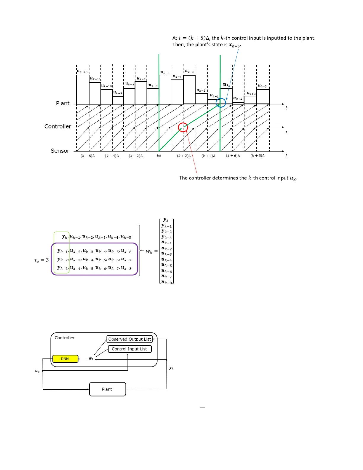
Network ed Contr ol of Nonlinear Systems under Partial Obser vation Using Continuous Deep Q-Learning Junya Ikemoto and T oshimitsu Ushio Abstract — In this paper , we pr opose a design of a model-free networked controller f or a nonlinear plant whose mathematical model is unknown. In a networked control system, the controller and plant are located away fr om each other and exchange data over a netw ork, which causes network delays that may fluctuate randomly due to network routing. So, in this paper , we assume that the current network delay is not known b ut the maximum value of fluctuating network delays is kno wn befor ehand. Mor eover , we also assume that the sensor cannot observe all state variables of the plant. Under these assumption, we apply continuous deep Q-learning to the design of the networked controller . Then, we introduce an extended state consisting of a sequence of past control inputs and outputs as inputs to the deep neural network. By simulation, it is shown that, using the extended state, the controller can learn a control policy rob ust to the fluctuation of the network delays under the partial observation. I . I N T RO D U C T I O N Reinforcement learning (RL) is one of theoretical frame- works in machine leaning (ML) and a dynamic programing- based learning approach to search of an optimal control policy [1]. RL is useful to design a controller for a plant whose mathematical model is unknown because RL is based on a model-free learning approach, that is, we can design the controller without plant’ s model. In RL, a controller that is a learner interacts with the plants and updates its control policy . The main goal of RL is to learn the control policy that maximizes the long-term rewards. RL has been applied to various control problems [2]-[8]. Furthermore, to design a controller for a complicated system, we often use function approximations. It is known that policy gradient methods [9], [10] with function approx- imations are especially useful in control problems, where states of plants and control inputs are continuous values. Recently , deep reinforcement learning (DRL) has been ac- tiv ely researched. In DRL, we combine con ventional RL algorithms with deep neural networks (DNNs) as high- performance function approximators [11]-[14]. In [15], DRL is applied to a parking problem of a 4-wheeled vehicle that is a nonholonomic system. In [16], DRL is applied to controlling robot manipulators. Moreov er , applications of DRL to networked control systems (NCSs) ha ve also been proposed [17], [18], [20]. NCSs have been much attention This work was partially supported by JST -ERA TO HASUO Project Grant Number JPMJER1603, Japan and JST -Mirai Program Grant Number JPMJMI18B4, Japan. J. Ikemoto and T . Ushio are with the Graduate School of Engineering Science, Osaka Univ ersity , T oyonaka, Osaka, 560- 8531, Japan ikemoto@hopf.sys.es.osaka-u.ac.jp ushio@sys.es.osaka-u.ac.jp to thanks to the dev elopment of network technologies. In NCSs, the controller and the plant are located away from each other . The controller computes control inputs based on outputs observ ed by the sensor , and sends them to the plant via a network. In [17], DRL is applied to control- aware scheduling of NCSs consisting of multiple subsystems operating over a shared network. In [18], DRL is applied to ev ent trigger control (ETC) [19]. Ho wev er , in [17] and [18], transmission delays over the network are not considered. One of the problems of NCSs is that there are network delays in the e xchange of data between the controller and the plant. In the case where the network delays are constant and parameters of the network delays are kno wn, we can design the networked controller considering the network delays. Howe ver , practically , it is difficult to identify the network delays beforehand. Moreov er , the network delays may fluctuate due to the network routing. Thus, in [20], we assume that the sensor can observe all state v ariables of the plant and proposed the design of network ed controller with network delays using a DRL algorithm. In general, howe ver , the sensor cannot always observe all of them. In RL, the partial observation often degrades learning performances of the controllers. In this paper, we consider the following networked control system; • The plant is a nonlinear system whose mathematical model is unknown. • Network delays fluctuate randomly due to the network routing, where the maximum value of them is known beforehand. • The sensor cannot observ e all state v ariables of the plant. Under the abov e assumptions, we propose a networked controller with a DNN using the continuous deep Q-learning algorithm [13]. Then, we introduce an extended state con- sisting of both past control inputs and outputs of the plant as inputs to the DNN. The paper is organized as follows. In Section II, we revie w continuous deep Q-learning. In Section III, we propose a networked controller using a DNN under the above three assumptions. In Section IV , by simulation, we apply the proposed learning algorithm to a network ed controller for stabilizing a Chua circuit under the fluctuating network delays and the partial observation. In Section V , we conclude the paper . I I . P R E L I M I N A R I E S This section re views RL and continuous deep Q-learning that is one of DRL algorithms. A. Reinfor cement Learning (RL) The main goal of RL is for a controller to learn its optimal control policy by trial and error while interacting with a plant. Let X and U be the sets of states and control inputs of the plant, respecti vely . The controller receiv es the immediate rew ard r k by the following function R : X × U × X → R . r k = R ( x x x k , u u u k , x x x k + 1 ) , (1) where x x x k and u u u k are the state and the control input at discrete- time k ∈ N . In RL, it is necessary to ev aluate the policy based on long-term re wards. Thus, the value function and Q-function are defined as follows. V µ ( x x x ) = E " ∞ ∑ n = 0 γ n r n + k | x x x k = x x x # , (2) Q µ ( x x x , u u u ) = E " ∞ ∑ n = 0 γ n r n + k | x x x k = x x x , u u u k = u u u # , (3) where µ : X → U is the ev aluated control policy , that is, the input u u u at the state x x x is determined by u u u = µ ( x x x ) , and γ ∈ [ 0 , 1 ) is the discount factor to pre vent the di ver gence of the long-term rew ards. In the Q-learning algorithm, the controller indirectly learns the following greedy deterministic polic y µ through updating the Q-function. µ ( x x x k ) = arg max u u u ∈ U Q ( x x x k , u u u ) . (4) B. Continuous Deep Q-learning with Normalized Advantage Function T o implement the Q-learning algorithm for plants whose state and control input are continuous, Gu et al . proposed a parameterized quadratic function A ( x x x , u u u ; θ ) , called a normal- ized advantage function (NAF) [13], satisfying the following equations, where θ is a parameter vector of the DNN. Q ( x x x , u u u ; θ ) = V ( x x x ; θ ) + A ( x x x , u u u ; θ ) , (5) A ( x x x , u u u ; θ ) = − 1 2 ( u u u − µ ( x x x ; θ )) T P ( x x x ; θ )( u u u − µ ( x x x ; θ )) , (6) where P ( x x x ; θ ) is a positive definite matrix and V ( x x x ; θ ) and Q ( x x x , u u u ; θ ) are approximaitors to Eqs. (2) and (3), respec- tiv ely . µ ( · ; θ ) computes the optimal control input instead of Eq. (4), where the control input maximizes the approxi- mated Q-function Q ( x x x , u u u ; θ ) instead of Eq.(3). In the other words, the approximated Q-function is di vided into an action- dependent term and an action-independent term, and the action-dependent term is expressed by the quadratic function with respect to the action. From Eqs. (5) and (6), when u u u = µ ( x x x ; θ ) , the Q-function is maximized with respect to the action u u u ∈ U and we have V ( x x x ; θ ) = max u u u ∈ U Q ( x x x , u u u ; θ ) . (7) Fig. 1. Illustration of a DNN for the continuous deep Q-learning with a N AF . The DNN outputs the approximated value V ( x x x ; θ ) , the optimal action µ ( x x x ; θ ) , and the parameters of the NAF for the inputted state x x x . Fig. 2. Block diagram of NCSs problem in which the network delays are caused by transmissions of control inputs and observed outputs. W e show an illustration of a DNN for continuous deep Q-learning in Fig. 1. The outputs of the DNN consist of the approximated value V ( x x x ; θ ) , the optimal control input µ ( x x x ; θ ) , and the parameters that constitute the lower trian- gular matrix L ( x x x ; θ ) , where the diagonal terms are exponen- tiated. Moreover , the positiv e definite matrix P ( x x x ; θ ) is giv en by L ( x x x ; θ ) L ( x x x ; θ ) T . I I I . C O N T I N U O U S D E E P Q - L E A R N I N G - B A S E D N E T W O R K C O N T R O L A. Networked Contr ol System W e consider the networked control of the following non- linear plant as shown in Fig. 2. ˙ x x x ( t ) = f ( x x x ( t ) , u u u ( t )) , (8) y y y k = h ( x x x ( k ∆ )) , (9) where • x x x ( t ) ∈ X ⊆ R n is the state of the plant at time t ∈ R , • u u u ( t ) ∈ U ⊆ R m is the control input of the plant at time t ∈ R and the k -th updated control input computed by the digital controller is denoted by u u u k , • y y y k ∈ Y ⊆ R p ( p < n ) is the k -th output of the plant observed by the sensor , • ∆ is the sampling period of the sensor , • f : R n × R m → R n describes the mathematical model of the plant, but it is assumed to be unkno wn, and • h : R n → R p is the output function of the plant that is characterized by the sensor . The discrete-time control input u u u k is sent to the D/A con- verter and held until the next input is received. The plant and the digital controller are connected by information networks and there are two types of network delays: One is caused by transmissions of the observed outputs from the sensor to the controller while the other is by those of the updated control inputs from the digital controller to the plant. The former and the latter delay at discrete-time k are denoted by τ sc , k and τ c p , k , respectively . Then, for k ∆ + τ sc , k + τ c p , k ≤ t < ( k + 1 ) ∆ + τ sc , k + 1 + τ c p , k + 1 , u u u ( t ) = u u u k . (10) W e assume that the packet loss does not occur in the networks and all data are receiv ed in the same order as their sending order . W e assume that both network delays are upper bounded and the maximum v alues of them are known beforehand. B. Extended State W e assume that the maximum values of τ sc , k and τ c p , k are known and let max ( τ sc , k ) = a ∆ and max ( τ c p , k ) = b ∆ ( a , b ∈ N and a + b = τ ). First, we consider randomly fluctuated delays. The sensor observes the k -th output y y y k at t = k ∆ . The controller receiv es the k -th output y y y k and computes the k -th control input u u u k at t = k ∆ + τ sc , k . The k -th control input u u u k is inputted to the plant at t = k ∆ + τ sc , k + τ c p , k . Then, the controller must estimate the state x x x ( k ∆ + τ sc , k + τ c p , k ) and compute u u u k . Since τ sc , k + τ c p , k ≤ τ ∆ , we use the last τ control inputs that the controller needs in the worst case to estimate the state of the plant as shown in Fig. 3. Thus, in [20], we introduced the extended state z z z k = [ x x x k , u u u k − 1 , u u u k − 2 , ..., u u u k − τ ] T and use it as the input of a DNN. W e also use the past control input sequence. Howe ver , in this paper , the sensor cannot observe all state variables x x x k . Second, we consider a partial observation. In [21], Aangenent et al. proposed a data-based optimal con- trol method using past control input and output se- quence in the case where the plant is a linear , control- lable, and observable system. Then, the length of the se- quence must be larger than the observability index K of the plant, where K ≤ n ≤ K p . Similarly , in this paper, we also use the past control input and output sequence { y y y k − 1 , y y y k − 2 , ..., y y y k − τ o , u u u k − ( τ + 1 ) , u u u k − ( τ − 2 ) , ..., u u u k − ( τ + τ o ) } to estimate the state x x x k as shown in Fig. 4, where the hyper parameter τ o ∈ N is selected beforehand. Although there is no theoretical guarantee, we select τ o conservati vely such that τ o ≥ n . W e define the following extended state w w w k . w w w k =             y y y k . . . y y y k − τ o u u u k − 1 u u u k − 2 . . . u u u k − ( τ + τ o )             ∈ R p τ o + m ( τ + τ o ) . (11) Thus, we design the networked controller with a DNN as shown in Fig. 5. Algorithm 1 Continuous Deep Q-learning with the N AF and the τ -extended state of the networked control systems 1: Select the length of the past output sequence τ 0 2: Initialize the replay memory D . 3: Randomly initialize the main Q network with weights θ . 4: Initialize the target network with weights θ − = θ . 5: for episode = 1 , ..., M do 6: Initialize the initial state x x x 0 ∼ p ( x x x 0 ) . 7: Receiv e the initial observed output y y y 0 . 8: Memorize the observed output y y y 0 . 9: Generate the initial extended state w w w 0 , where u u u i = 0 ( i < 0 ) . 10: Initialize a random process N for action exploration. 11: for k = 0 , ..., K do 12: if k > 0 then 13: Receiv e the k -th output y y y k . 14: Memorize the observed output y y y k . 15: Generate the extended state w w w k with past control inputs and outputs. 16: Return the rew ard r k − 1 = R ( w w w k − 1 , u u u k − 1 , w w w k ) . 17: Store the transition ( w w w k − 1 , u u u k − 1 , w w w k , r k − 1 ) in D . 18: end if 19: Determine the control input u u u k = µ ( w w w k ; θ ) + N k and send the control input to the plant. 20: Memorize the control input u u u k . 21: if k % k p = 0 then 22: for iteration = 1 , ..., I do 23: Sample a random minibatch of N transitions ( w w w ( n ) , u u u ( n ) , w w w 0 ( n ) , r ( n ) ) , n = 1 , ..., N from D . 24: Set t ( n ) = r ( n ) + γ V ( w w w 0 ( n ) ; θ − ) . 25: Update θ by minimizing the loss: J ( θ ) = 1 N ∑ N n = 1 ( t ( n ) − Q ( w w w ( n ) , u u u ( n ) ; θ )) 2 . 26: Update the target network: θ − ← β θ + ( 1 − β ) θ − . 27: end for 28: end if 29: end for 30: end f or C. DRL algorithm The parameter vector of the DNN for the controller is optimized by the continuous deep Q-leaning algorithm [13]. Fig. 3. W e consider the case where max ( τ sc , k ) = 2 ∆ and max ( τ c p , k ) = 3 ∆ . If the all network delays are maximum, the controller needs the past control input sequence { u u u k − 1 , u u u k − 2 , ..., u u u k − 5 } to estimate x x x k + 5 and compute the k -th control input u u u k . Fig. 4. In the case where the sensor cannot observe all state variables of the plant, we use past control inputs and outputs as the extended state. For example, we set τ o = 3. Then, we use the past control inputs { u u u k − 1 , u u u k − 2 , ..., u u u k − 8 } and outputs { y y y k − 1 , y y y k − 2 , y y y k − 3 } as the extended state w w w k . Fig. 5. The network controller is designed with a DNN. When the controller receiv es the k -th observed output y y y k at t = k ∆ + τ sc , k , it computes the k -th control input u u u k based on the extended state w w w k . Then, the input of the DNN is w w w k . The parameter vector of the deep neural network for the controller is optimized by the continuous deep Q-leaning algorithm [13]. The input to the DNN is the extended state w w w k . Shown in Algorithm 1 is the proposed learning algorithm. In the same way as the DQN algorithm [11], we use the experience replay and the target network. The parameter vectors of the main network and the target network are denoted by θ and θ − , respectiv ely . For the update of θ , the following TD error is used. J ( θ ) = ( t k − Q ( w w w k , u u u k ; θ )) 2 , (12) t k = r k + γ V ( w w w k ; θ − ) . (13) Moreov er , for the update of θ − , the follo wing soft update is used. θ − ← β θ + ( 1 − β ) θ − , (14) where β is giv en as a very small positiv e real number . The exploration noises N k ( k = 1 , 2 , ... ) are generated under a giv en random process N . I V . S I M U L A T I O N W e apply the proposed controller to a stabilization of a Chua circuit as follows. W e set the sampling period to ∆ = 2 − 4 ( s ) . Moreover , we assume that the terminal of a leaning episode is at t = 12 . 0 ( s ) . A. Chua cir cuit The dynamics of a Chua circuit is gi ven by d d t   x ( t ) y ( t ) z ( t )   =   p 1 ( y ( t ) − φ ( x ( t ))) x ( t ) − y ( t ) + z ( t ) + u ( t ) − p 2 y ( t )   , (15) where φ ( x ) = ( 2 x 3 − x ) / 7. In this simulation, we assume that p 1 = 10 and p 2 = 100 / 7, where these parameters are Fig. 6. The trajectory of a Chua circuit is depending on an initial state. (a) The initial state is [ − 0 . 2 , 0 . 1 , − 0 . 1 ] and its behavior conv erges to a chaotic attractor . (b) The initial state is [ 2 . 0 , − 1 . 0 , 1 . 0 ] and its behavior conv erges to a limit cycle. unknown. The Chua circuit has a chaotic attractor and a limit cycle as shown in Fig. 6. W e assume that the states x and y are sensed as follows. y y y k =  1 0 0 0 1 0    x ( k ∆ ) y ( k ∆ ) z ( k ∆ )   . (16) W e assume that equilibrium points of the Chua circuit is unknown because the controller does not know the parame- ters p 1 and p 2 . Thus, we define the rew ard function in this simulation as follows. First, we define the reward r ( 1 ) k based on outputs y y y k , y y y k + 1 and the control input u k . r ( 1 ) k = − ( y y y k + 1 − y y y k ) T  0 . 8 0 0 0 . 8  ( y y y k + 1 − y y y k ) − 1 . 0 u 2 k . (17) Second, we define the reward based on the past output sequence used for the extended state. r ( 2 ) k = − τ o ∑ i = 1  ( y y y k + 1 − i − y y y k − i ) T  0 . 8 0 0 0 . 8  ( y y y k + 1 − i − y y y k − i )  . (18) Third, we define the reward based on the past control input sequence used for the extended state. r ( 3 ) k = − 0 . 15 τ + τ o ∑ i = 1 ( u k + 1 − i − u k − i ) 2 . (19) Finally , we define the immediate reward at discrete-time k as follows. r k = r ( 1 ) k + r ( 2 ) k + r ( 3 ) k . (20) Thus, the goal of DRL is the stabilization of the circuit at one of equilibrium points. Fig. 7. Learning curve. For all k , ∆ ≤ τ sc , k ≤ 3 ∆ and ∆ ≤ τ c p , k ≤ 3 ∆ . The values of the vertical axis are gi ven by the sum of r k between the 50th sampling and the episode’s terminal for each episode. B. Design of the contr oller W e use a DNN with four hidden layers, where all hidden layers hav e 128 units and all layers are fully connected layers. The acti vation functions are ReLU except for the output layer . Regarding the activ ation functions of the output layer , we use a linear function for both the V unit and units for parameters of the adv antage function, while we use a weighted hyperbolic tangent function for the µ unit. The size of the replay memory is 1 . 0 × 10 6 and the minibatch size is 128. The parameters of the DNN are updated 10 times per 4 discrete time steps ( I = 10 , k p = 4) by ADAM [22], where its learning stepsize is 1 . 25 × 10 − 5 . The soft update rate β for the target network is 0.001, and the discount rate γ for the Q-value is 0.99. For the exploration noise process, we use an Ornstein- Uhlenbeck process [23]. The exploration noises are multi- plied by 3.5 during the 1st to the 1000th episode, and the noise is gradually reduced after the 1001st episode. The initial state is randomly selected for each episode, where − 4 . 5 ≤ x ( 0 ) ≤ 4 . 5, − 4 . 5 ≤ y ( 0 ) ≤ 4 . 5, and − 4 . 5 ≤ z ( 0 ) ≤ 4 . 5. C. Result First, we assume that, for all k ∈ N , the network delays are set to ∆ ≤ τ sc , k ≤ 3 ∆ and ∆ ≤ τ c p , k ≤ 3 ∆ . These ranges are unknown. Ho we ver , we assume that we know max ( τ sc , k ) = 4 ∆ and max ( τ c p , k ) = 4 ∆ beforehand. Thus, we set τ = 8. Moreov er , we select τ o = 4, that is, τ o is larger than the dimension of the plant’ s state ( n = 3). The learning curv e is sho wn in Fig. 7, where the v alues of the vertical axis, called re wards, are gi ven by the sum of r k between the 50th sampling and the episode’ s terminal for each episode. It is sho wn that the controller can learn a control policy that achiev es a high reward. Moreov er , shown in Figs. 8 and 9 are the time responses of the Chua circuit using the control policy after 8500 episodes. It is sho wn that the controller that sufficiently learned the control policy using the proposed method can stabilize the circuit. V . C O N C L U S I O N In this paper, we proposed a model-free networked con- troller for a nonlinear plant with network delays using Fig. 8. Time response of the Chua circuit using a control policy after 8500 episodes. For all k , ∆ ≤ τ sc , k ≤ 3 ∆ and ∆ ≤ τ c p , k ≤ 3 ∆ . The parameter τ is set to 8 and the parameter τ o is set 4. The initial state is [ − 0 . 2 , 0 . 1 , − 0 . 1 ] , where its conv erged behavior is shown in Fig. 6(a). continuous deep Q-learning. Moreov er , the sensor cannot observe all state variables of the plant. Thus, we introduce an extended state consisting of a sequence of the past control inputs and outputs and use it as an input to a DNN. W e showed the usefulness of the proposed controller by stabilizing a Chua circuit. It is future work to e xtend the proposed controller under the existence of packet loss and sensing noises. R E F E R E N C E S [1] R. S. Sutton and A. G. Barto, “Reinforcement Learning: An Introduc- tion, ” Bradford Book. MIT Pr ess, Cambridge, Massachusetts, 1999. [2] F . L. Lewis and D. Vrabie, “Reinforcement Learning and Adaptiv e Dynamic Programming for Feedback Control, ” IEEE Circuits and Systems Magazine, vol. 9, no. 3, pp. 3250, 2009. [3] F . L. Lewis and D. Liu, “Reinforcement Learning and Approximate Dynamic Programming for Feedback Control, ” IEEE Pr ess, 2013. [4] F . L. Lewis and K. G. V amvoudakis, “Reinforcement Learning for Partially Observable Dynamic Processes: Adaptive Dynamic Program- ming Using Measured Output Data, ” IEEE T rans. Systems, Man, and Cybernetics. P art B-Cybernetics, vol. 41, no. 1, pp. 1425, 2011. [5] T . Fujita and T . Ushio, “RL-based Optimal Networked Control Con- sidering Networked Delay of Discrete-time Linear Systems, ” in Proc. of 2015 IEEE ECC, pp. 2481-2486, 2015. [6] T . Fujita and T . Ushio, “Optimal Digital Control with Uncertain Network Delay of Linear Systems Using Reinforcement Learning, ” IEICE T rans. Fundamanetals, vol. E99-A no. 2, pp. 454-461, 2016. [7] E. M. W olff, U. T opcu, and R. M. Murray , “Robust Control of Uncer- tain Markov Decision Processes with T emporal Logic Specications, ” in Pr oc. of 2012 IEEE CDC, pp. 3372-3379, 2012. [8] M. Hiromoto and T . Ushio, “Learning an Optimal Control Policy for a Markov Decision Process Under Linear T emporal Logic Specications, ” in Pr oc. of IEEE Symposium Series on Computational Intelligence, pp. 548-555, 2015. [9] R. S Sutton, D. McAllester, S. Singh, and Y . Mansour, “Policy Gradient Methods for Reinforcement Learning with Function Approx- imation, ” in Proc. of the 12th NIPS, pp. 1057-1063, 1999. [10] D. Silver , G. Lever , N. Heess, T . Degris, D Wierstra, and M. Ried- miller , “Deterministic Policy Gradient Algorithms, ” in Pr oc. of the 31st ICML, vol. 32, pp. 387-395, 2014. Fig. 9. Time response of the Chua circuit using a control policy after 8500 episodes. For all k , ∆ ≤ τ sc , k ≤ 3 ∆ and ∆ ≤ τ c p , k ≤ 3 ∆ . The parameter τ is set to 8 and the parameter τ o is set to 4. The initial state is [ 2 . 0 , − 1 . 0 , 1 . 0 ] , where its conv erged behavior is shown in Fig. 6(b). [11] V . Mnih, K. Ka vukcuoglu, D. Silve, A. A. Rusu, J. V eness, M. G. Bellemare, A. Graves, M. Riedmiller, A. K. Fidjeland, G. Ostrovski, S. Petersen, C. Beattie, A. Sadik, I. Antonoglou, H. King, D. K umaran, D. Wierstra, S. Legg, and D. Hassabis, “Human-Level Control through Deep Reinforcement Learning, ” Nature , vol. 518, pp. 529-533, 2015. [12] T . P . Lillicrap, J. J. Hunt, A. Pritzel, N. Heess, T . Erez, Y . T assa, D. Sil- ver , and D. W ierstra, “Continuous Control with Deep Reinforcement Learning, ” arXiv preprint arXiv:1509.02971, 2016. [13] S. Gu, T . Lillicrap, I. Sutske ver , and S. Levine, “Continuous Deep QLearning with Model-based Acceleration, ” in Proc. of the 33r d ICML, pp. 2829-2838, 2016. [14] V . Mnih, A. P . Badia, M. Mirza, A. Grav es, T . Harley , T . P . Lillicrap, D. Silver, and K. Kavukcuoglu, “ Asynchronous Methods for Deep Reinforcement Learning, ” in Proc. of the 33rd ICML, pp. 1928-1937, 2016. [15] N. Masuda and T . Ushio, “Control of Nonholonomic V ehicle Sys- tem Using Hierarchical Deep Reinforcement Learning, ” in Proc. NOLT A2017, pp. 26-29, 2017. [16] B. Sangiovanni, G. P . Incremona, A. Ferrara, and M. Piastra, “Deep Reinforcement Learning Based Self-Conguring Integral Sliding Mode Control Scheme for Robot Manipulators, ” in Proc. of 2018 IEEE CDC, pp. 5969-5974, 2018. [17] B. Demirel, A. Ramaswamy , D. E. Quevedo, and H. Karl, “Deep- CAS: A Deep Reinforcement Learning Algorithm for Control-A ware Scheduling, ” IEEE Contr ol System Letters, vol. 2, no. 4, pp. 737-742, 2018. [18] D. Baumann, J-J. Zhu, G. Martius, and S. Trimpe, “Deep Reinforce- ment Learning for Event-Triggered Control, ” in Proc. of 2018 IEEE CDC, pp. 943-950, 2018. [19] W . P . M. H. Heemels, K. H. Johansson, and P . T abuada, “ An Intro- duction to Event-Triggered and Self-T riggered Control, ” in Pr oc. of 2012 IEEE CDC, pp. 32703285, 2012. [20] J. Ikemoto and T . Ushio, “ Application of Continuous Deep Q-Learning to Networked State-Feedback Control of Nonlinear Systems with Uncertain Network Delays, ” in Pr oc. NOLT A2019, 2019. [21] W . Aangenent, D. Kostic, B. de Jager, R. van de Molengraft, and M. Steinbuch, “Data-Based Optimal Control, ” in Proc. of 2005 IEEE ACC, pp. 1460-1465, 2005. [22] D. P . Kingma and J. L. Ba, “ ADAM: A Method for Stochastic Operation, ” arXiv preprint arXiv:1412.6980, 2014. [23] G. E. Uhlenbeck and L. S. Ornstein, “On the Theory of the Brownian Motion, ” Physical revie w , vol. 36, no. 5, pp. 823-841, 1930.