Dissipativity analysis of negative resistance circuits

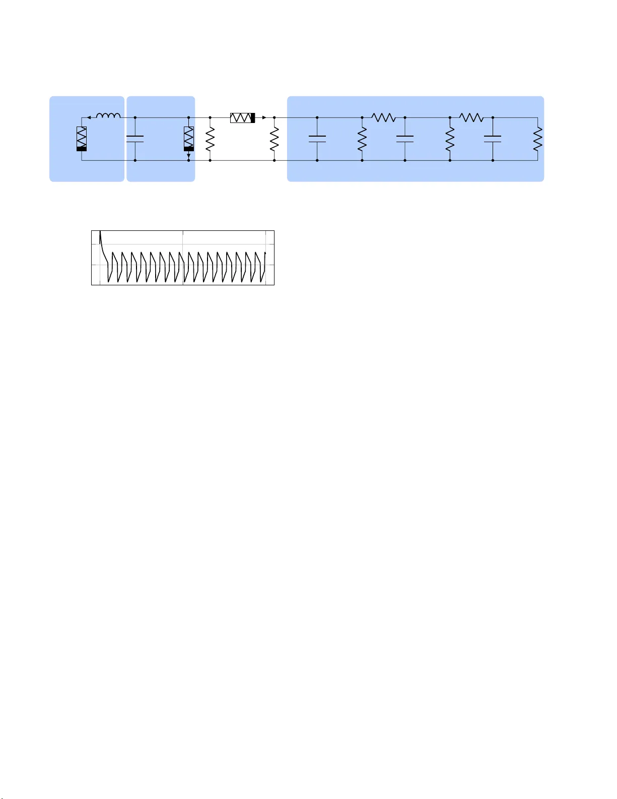
Dissipati vit y analysis of neg ativ e res istance ci rcuits F ´ elix A. Mir anda-Vi llat oro a , F ulvio F orni a , Ro dolphe Sepulc hre a a University of Cambridge, Dep artment of Engine ering. T ru mpi ngton Str e et, Cambridge, CB2 1PZ. Abstract This pap er deals with the an alysis of nonlinear circuits that interconnect passiv e elements (capacitors, inductors, and resistors) with nonlinear resistors exhibiting a range of ne gative resistance. Su ch active elements are necessary to design circuits that switc h and os cillate. W e generalize the classical passivit y theory of circuit analysis to account for suc h non-equilibrium behaviors. The approach closely mimics the classical metho dology of (incrementa l) dissipativit y t heory , but with d issipation inequalities that combine signe d storage functions and signe d supply rates to accoun t for the mix ture of passive and activ e elements. Key wor ds: Nonlinear circuits; Dissipative systems; Active elements; Limit cycles; Bistabilit y . 1 In tro duction The c oncept of passiv it y is a foundation o f cir cuit theo r y [1]. It led to the generalized concept of dissipativity [35], [36], which has b ecome a founda tion of nonlinear sy stem theory [18,33]. Y et the applica tions of no nlinear system theory ha ve b een dominated by mechanical a nd electro- mechanical s ystems [6], [12], [27], [30], with significantly less a tten tion to nonlinear circuits [5,7]. Starting with the seminal work of Chua [9] and the tex t- bo ok of Ch ua and Deso er [10], the r esearch on nonlin- ear cir cuits has somewhat diverged from the resear ch on nonlinear dissipative systems. The e mphasis in nonlin- ear circuit theor y has be e n on non-equilibr ium behaviors whereas the fo cus of dissipativity theory is an intercon- nection framework fo r systems that conv erg e to equilib- rium. Negative resistance devices are the essence of non- equilibrium behaviors suc h as switches [8], [17], [22], nonlinear oscillatio ns [1 9], [23], or c hao tic behavior [21], [29]. In contrast, dissipativity theory is a stability the- ory for physical systems that only dissipate ener gy and that relax to equilibrium when disconnected from a n external source of energy . ⋆ The researc h leading to these results has receiv ed funding from the Europ ean Researc h Council un der the Advanced ERC Gran t Agreement Switchlet n.670645. Email addr esses: fam48@cam.ac.uk (F´ elix A. Miranda-Villatoro), f.forni@ eng.cam.ac.uk (F ulvio F orni), r.sepulchre@e ng.cam.ac.uk (R od olphe Sep ulchre). The present pa pe r is a step tow ards generalizing pa ssiv- it y theory to the analysis of negative resis ta nce cir cuits. In the spirit of passivity theor y , we seek to analyze non- linear circuits through dissipation inequalities that are preserved b y in terco nnection. The tw o basic elements o f dissipativity theory ar e the storage function and the supply function. A dissipative system ob eys a dissipation inequa lity , which expresses that the r a te of change of the stora ge do es not exceed the s upply . The physical interpretation is that the sto r- age is a measur e of the internal energy , whereas the in- tegral of the supply is a measur e of the supplied energy . F or stability analysis purp oses, the storage b ecomes a Lyapuno v function. The approach in this pap er is bas ed on t wo mo difica tions of the basic theory . Fir s t, the a nalysis is in terms of incr emental v aria bles, that is, differences o f voltages and currents r ather than voltages and currents. Incr ement al analysis is classical in no nlinear circuit theory . Star ting with the seminar work of [24], incre men tal a na lysis has also been increasingly used in nonlinear stability theory [2], [13], and in no nlinear dissipativity theo ry [16], [28], [31], [34]. Seco nd, we allow for dissipatio n inequalities that combine signe d stor age functions a nd signe d s upply rates. Signed storage functions hav e the interpretation of a difference of energ y stored in different storag e ele ments whereas sig ned supply rates account for p or ts that can deliver rather than absor b energ y . F or analysis purp oses, the interconnection theo ry de- veloped in the present paper makes contact with the dominance theor y recently prop osed in [14], [1 5]. Signed Preprint submitted to Au tomatica 30 Au gust 2019 Lyapuno v functions with a restricted num b er o f negative terms are used to prov e conv erge nc e to low-dimensional dynamics that do minate the asymptotic b ehavior. A one-dimensional dominant behavior is sufficien t to mo del bistable switc hes whereas a tw o -dimensional dominant b ehavior is sufficient to mo del nonlinear os- cillators. Co mbin ed with the interconnection theo ry of this pap er, do minance theory o pens the wa y to analy s is of nonlinea r switches and nonlinear oscillator s in la rge nonlinear circuits. W e deliber a tely restrict the scop e of the pre s ent pa p er to nonlinear c ir cuits w ith negative r esistance to facilitate a concrete interpretation o f the results. Not surpr isingly , the co ncepts are no t restr icted to electrical circuits and hav e a more gener al interpretation in the general frame- work of dissipativity theor y . F or c o ncreteness, the entire pap er is r estricted to the pa ssivity supply , an inner pro d- uct betw een cur r ents and voltages, with the conv enient int erpr etation o f electrica l power. The paper is org anized as follows. Section 2 dea ls with the dis s ipation prop erties of nega tive resistance devices and Section 3 ex tends dominance theory in an inc r emen- tal fra mework that is suitable for the a nalysis o f circuits with piecewise linear characteristics. In Section 4 w e an- alyze ba sic electrical switches and oscillato rs with one or t wo s torage elements, wherea s Section 5 cov ers the de- sign of coupling netw or ks that allows us to in terconnect circuits with different s ig natures in the supply r a tes. Preamble. The circuits stu died in this pap er are built from interco nn ec- tions of li ne ar p assive elemen ts, such as capacitors and in- ductors, and nonline ar act ive resistors. In concrete, the time evol ution of the family of circuits studied here is describ ed by the state-space mo del Σ : ( ˙ x = f ( x ) + B u x (0) = x 0 y = C x + Du (1) where x ∈ R n is the state of the system and u, y ∈ R m are the so-called manifest v ariables. F or electrical circuits, th e manifest v ariables are conjugated in t erms of voltages v , and currents i , that is, the inn er pro duct u ⊤ y has units of pow er. The map f : R n → R n is Lipsc hitz contin uous and mo dels intera ctions b etw een linear storage elements and nonlinear resistors. Moreo ver, the matrices B , C , and D are of the ap- propriate d imensions and such th at the system is well-posed. Henceforth, every circuit in this pap er is assumed to b e of the form (1). In what follo ws we will adopt a differ ential (or incremental ) approach, that is, we will study circuit prop- erties by looking at the difference b etw een tra jectories. F or simplicit y , w e denote the difference b etw een any tw o generic signals w 1 , w 2 as ∆ w := w 1 − w 2 . In this wa y , the mismatches b etw een an y t wo states/currents/v oltages are d enoted as ∆ x , ∆ i and ∆ v resp ectivel y . Finally , we will use symmetric ma- trices P ∈ R n × n constrained to hav e inertia ( p, 0 , n − p ), that is, with p negative eigenv alues and n − p p ositiv e eigenv alues. 2 Signed supply rates for nonlinear resi stors The nonlinear element s hown in Figur e 1 is a funda- men tal element of nonlinear circuits. The voltage range where the nonlinear c har a cteristic has a neg a tive slop e mo dels an element that can deliver energy rather than dissipating ener gy . Such an element is called active in contrast to p assive ele ments that can only absorb en- ergy . W e follow the common terminology of ne gative r e- sistanc e device [11], [20], with the usual caveat that ne g- ative refers to the incr ement ∆ v rather than to the v alue of the voltage v . A mor e precis e (but also heavier) termi- nology w ould be ne gative incr emental (or differ ential) re- sistance. The ana lysis in this pa p er will be exclusively in terms of incr emental quantities, which is common prac- tice in nonlinear circuit theory . i − + v 0 v v 0 i i G d − G g v [ V ] i [ A ] Fig. 1. Slope-b ounded vol tage-current c haracteristic of a tu n- nel diod e. T u nnel dio des are (incrementally) negativ e resis- tance devices. The region of negativ e slop e is called the ac- tive region. W e are motiv ated by the prop erty that this no nlinear element satisfies the tw o inequalities 0 ≤ ∆ i ∆ v + G g (∆ v ) 2 (2a) 0 ≤ − ∆ i ∆ v + G d (∆ v ) 2 (2b) where G d > 0 and − G g < 0 repr esent, resp ectively , the maximum p os itive slop e and negative slo p e of the voltage-current characteristic of Figure 1 . Bo th inequal- ities have an obvious energetic interpretation: the fir st inequality express es the sho rtage of pa s sivity of the el- ement : the element becomes pass ive when connected in parallel with a r esistor of r esistance les ser than 1 /G g . The second inequality expres ses the shorta ge of anti- passivity of the element: the element b ecomes purely a source of energy when connected to a nega tive resistance larger than − 1 /G d . In the language of dissipa tivity theory [35], b oth inequal- ities are dis s ipation inequalities of the form σ (∆ i, ∆ v ) ≥ 0 for the family of quadra tic supply rates σ (∆ i, ∆ v ) = " ∆ i ∆ v # ⊤ " Q I I R # " ∆ i ∆ v # (3) 2 where the signature matrix I ∈ R m × m is a di- agonal ma trix with ± 1 in the main diagonal I = Diag[ ± 1 , ± 1 , . . . , ± 1 ], a nd Q ∈ R m × m , R ∈ R m × m are symmetric matrices. In the specia l case I = I , this fam- ily of s upply ra tes characterize incr ementally pa ssive elements with an excess or a sho rtage of pass ivity in the external v a riables [30]. When Q = 0, the dissipativity prop erty σ (∆ i, ∆ v ) ≥ 0 is also equiv alent to the mono- tonicity o f the voltage-curr ent characteris tic i = g ( v ) [3]. The ma p g is called strong ly monotone for R > 0, hypomonotone for R < 0 and monotone for R = 0. W e call (3) a signe d passivity supply rate to stress that the only difference with respect to the conv entional pas - sivity supply is the signature matrix I g eneralizing the conv entional iden tity matrix I . The element in Figure 1 is called a voltage-co nt ro lled resistor, Figur e 2 (left). Namely , the current flowing through a voltage-controlled resistor is a singled-v alued function of the v oltage across its terminals: i = g ( v ). The nonlinear resistor is passive when the function g : R → R is monotone incre asing, otherwise it is active. It follows from (2) that whenever G d 6 = G g , a voltage-controlled resistor fulfills 0 ≤ " ∆ i ∆ v # ⊤ " Q I I R # " ∆ i ∆ v # (4) where I = sign( G d − G g ), Q = − 2 | G d − G g | and R = 2 G g G d | G d − G g | . The dual element is the current-con trolle d resistor de- fined b y a singled-v alued function o f its flowing curr ent: v = r ( i ). An active current-con tro lle d r esistor s a tisfies the s ector condition − R g (∆ i ) 2 ≤ ∆ i ∆ v ≤ R d (∆ i ) 2 (5) Equiv ale n tly , a curr ent-con trolled resistor sa tis fie s (4) with I = sign( R d − R g ), Q = 2 R g R d | R d − R g | and R = − 2 | R d − R g | . Both types of co ntrolled resisto rs ap- pea r naturally in devices suc h as tunnel dio des, DIA C’s or neon lamps. Additionally , they can b e built fro m off- the-shelf comp onents like tra nsistors and op era tional amplifiers [11], [20]. Describing nega tive resistor s in terms of dissipation in- equalities opens the wa y to the use of dissipativit y theory to characterize circuit interconnections. As an illustra- tion, consider the pa rallel interconnection of a voltage- controlled negative resista nce element with a capacitor (Figure 3 , left). Let i c , v c and i r , v r be the currents and voltages asso ciated to the capacito r and the controlled resistor, r esp ectively . The capacito r is a classical loss le s s R v c + − v g ( v ) R cc + − r ( i ) i Fig. 2. V oltage-controlled resistor (left) and current-con- trolled resistor (right). The funct ions g and r are assumed singled-v alued and Lipschitz contin uous. If g or r are mono- tone increasing then th e resistor is passive, otherwise it is active . element that satisfies the p ower-preserving equality d dt C (∆ v c ) 2 2 = ∆ v c ∆ i c (6) In the languag e of dis s ipativity theory , the quan tity on the left-hand side is the time-der iv ative o f the stor- age C (∆ v c ) 2 2 . The neg a tive resis tance element sa tis fies − ∆ v r ∆ i r + G d (∆ v r ) 2 ≥ 0. The parallel interconnection defined b y v cc = v c = v r and i cc = i c + i r 1 satisfies the dis s ipation (in)equality − d dt C (∆ v cc ) 2 2 ≤ − ∆ v cc ∆ i cc + G d (∆ v cc ) 2 (7) The quantit y that a ppe a rs on the left hand- s ide is the time-deriv a tive of a ne gative stor age. More gener ally , the storage functions in this pap er will b e quadratic forms defined by a s ymmetric matrix P = P T with p neg a- tive eigenv alues (a nd n − p p ositive eigenv a lues). Such signe d storage functions generalize the conv entional p osi- tive definite storag es of passivity theory . P os itive definite storage s are natur al candidates for the stability analysis of clos ed equilibrium systems. In its incr ement al for m, stability ana lysis app ear s in the literature under differ- ent names, including c ontr action theory [2 4], incr emen- tal stability analysis [2], or differential Lyapuno v analy- sis [13]. Signe d storage s generalize this s tability a nalysis for no n-equilibrium behaviors c hara cterized by a low- dimensional asymptotic b ehavior. This gener alization is the topic o f dominance analys is, r eviewed in the next section. 3 Different ial dissipativi ty 3.1 Dominant systems Dominance theo ry extends s tability analysis to non- equilibrium b ehaviors. The approach is based o n the 1 The superindices in the v ariables i cc and v cc indicate that the p ort under consideration is current-driven. In a similar w ay , i vc and v vc will denote th e v ariables associated to a vol tage-driven p ort. 3 L ξ R cc + − r ( ξ ) − + v v c i v c C + − x R v c g ( x ) i cc + − v cc Fig. 3. Basic prototyp e circuits of a current-driven (left) and a voltage-driv en (righ t) 1-passive circuit. The resistors R vc and R cc are voltage-con t rolled and curren t-controlled resistors resp ectively . int uitive idea that the lo ng run b ehavior of the sy s- tem is dictated by low-dimensional dynamics, iden tified through the study of the system lineariza tion [13], [14], [15]. In wha t follows we adapt the differential approa ch of [15] into an incremental setting. Definition 1 L et f : R n ⇒ R n b e a Lipschitz c ontinu- ous map. A system of the form ˙ x ∈ f ( x ) , x ∈ R n , (8) is p -dominant with r ate λ ≥ 0 if ther e exists a matrix P = P ⊤ ∈ R n × n with inertia ( p, 0 , n − p ) such that " ∆ ˙ x ∆ x # ⊤ " 0 P P 2 λP + εI # " ∆ ˙ x ∆ x # ≤ 0 . (9) The pr op erty is strict if ε > 0 . When P is p os itive definite, (9) b ecomes the incremental analogue o f the classical Lyapuno v inequality , meaning that any t wo tra jectories co nv erge to each other with decay rate at leas t λ ≥ 0, [4]. When f is a differ e ntiable map, (9) re duce s to the simple matrix inequality ∂ f ( x ) ∂ x ⊤ P + P ∂ f ( x ) ∂ x + 2 λP ≤ − εI , (10) which provides a basic test for do minance, [1 4 ], [15]. Theorem 2 L et f : R n → R n b e a differ entiable map. The close d system (8) is p -dominant if and only if, ther e exists a matrix P = P ⊤ with inertia ( p, 0 , n − p ) such that (10 ) holds. PR OOF. First assume that (8) is p -dominant. Expand- ing the left-hand side of (9) a nd dividing b y k ∆ x k 2 6 = 0 yields, ∆ f ⊤ P ∆ x + ∆ x ⊤ P ∆ f + 2 λ ∆ x ⊤ P ∆ x + ε ∆ x ⊤ ∆ x k ∆ x k 2 ≤ 0 . By le tting δ x = lim ∆ x → 0 ∆ x k ∆ x k we arr ive to (10). F or the conv erse statement, let x ( α ) = αx 1 + (1 − α ) x 2 and let φ : R → R b e such that φ ( α ) = 2 ( f ( x ( α )) − f ( x 2 ) + λ ( x ( α ) − x 2 )) ⊤ P ∆ x + ε ( x ( α ) − x 2 ) ⊤ ∆ x where ∆ x = x 1 − x 2 . Hence , dφ ( α ) dα = ∆ x ⊤ ∂ f ( x ) ∂ x ⊤ P + P ∂ f ( x ) ∂ x + 2 λP + εI  ∆ x ≤ 0 . The ab ov e inequa lity implies that φ is a non-increas ing function. Ther e fore, φ (1) ≤ φ (0) = 0 and (9) follows. This concludes the pro of. ✷ The prop e rty of dominance strong ly constrains the asymptotic b ehavior of the system as descr ibe d for the following theorem. Theorem 3 ([15, Theorem 2 ]) L et (8) b e strictly p - dominant with ra te λ ≥ 0 . F or any given x ∈ R n , let Ω( x ) b e t he ω - limit set of x . Then the flow of (8) on Ω( x ) is t op olo gic al ly e quivalent to the fl ow of a p -dimensional system. Additionally , the following co rollar y b ecomes useful in characterizing the asymptotic b ehavior of a dominant system. Corollary 4 Under the assu m ptions of The or em 3, ev- ery b ounde d t r aje ctory of (8) c onver ges to • A unique e quilibrium p oint if p = 0 . • An e quilibrium p oint if p = 1 . • A simple attra ctor if p = 2 . Summing up, c lo sed dynamic systems with smaller de- grees of do minance will show simpler b ehaviors com- pared with systems w ith higher degr ees. The following subsection e xtends the prop er ty of dominance to o pe n systems under the framework of diss ipa tive systems. 3.2 Signe d dissip ation ine qualities Dissipativity theory [35], [3 6] is grounded in dissipation inequalities, which generalize the physical characteriza- tion of a pas sive circuit a s a system that ca n only a bsorb energy: the v ariatio n o f energ y stor e d in the elements of the circuit (capacitors and inducto rs) is upper b ounded by the electrical p ower supplie d to the circuit. F or a linea r circuit, the storage is a quadra tic function o f the sta te, and the dissipation inequality takes the standard for m d dt x ⊤ P x ≤ − λx ⊤ P x + v ⊤ i + i ⊤ v 4 The scalar λ ≥ 0 determines a dissipation rate. Each pair of voltage v k and current i k app earing in the voltage vector v and voltage current i determines a p ort of the circuit. In matrix form, the quadratic dissipatio n inequality characterizing passivity reads " ˙ x x # ⊤ " 0 P P 2 λP # " ˙ x x # ≤ " v i # ⊤ " 0 I I 0 # " v i # (11) An incremental dissipation inequality is in term of the increments rather than abs o lute v a riables: " ∆ ˙ x ∆ x # ⊤ " 0 P P 2 λP # " ∆ ˙ x ∆ x # ≤ " ∆ v ∆ i # ⊤ " 0 I I 0 # " ∆ v ∆ i # (12) Motiv ated by the signed supply r ates and s igned storages int ro duce d in Section 2, w e gener alize the incremental passivity dissipatio n inequalit y (12) to signe d dissipation inequalities o f the form " ∆ ˙ x ∆ x # ⊤ " 0 P P 2 λP + εI # " ∆ ˙ x ∆ x # ≤ " ∆ v ∆ i # ⊤ " Q I I R # " ∆ v ∆ i # (13) for a n a rbitrary circuit with state x ∈ R n and m p or ts defining the curre nt i ∈ R m and v oltag e v ∈ R m . W e only consider circuits compo sed of linea r capacitors, linear inductors, and nonlinear resistors. The signe d quadratic storage is deter mined by the symmetric matrix P with p negative eigenv alue s and n − p p ositive eig env alues . The signe d supply is determined b y the signa ture matrix I . The scalar λ ≥ 0 is the dissipa tion ra te. The matrices Q , R are s ymmetric as in (3). Definition 5 A n online ar cir cuit is c al le d signe d p assive if the ine quality (13) hold s along any p air of tr aje ctories. The pr op erty is strict if ε > 0 . Definition 5 is v ery close to the classical definition of in- cremental passivity . The only difference is that (i) w e consider signe d storages, i.e. differ enc es of po s itive s to r- ages and (ii) signe d supply ra tes , i.e. differ enc es of the classical p assivity supply rates. As illustrated in Section 2, such storage s and s upply rates app ear na turally when considering cir cuits with b oth passive a nd active ele- men ts and ports that can b o th absor b a nd deliver energy . 3.3 Dissip ative inter c onne ct ions The central prop erty of pa s sivity theor y is tha t passiv - it y is preser ved by interconnection. More precisely , p ort int erco nnections of passive circuits are passive. In order to generalize this prop erty to signed-passivity , we in tro- duce the following definition. Definition 6 L et Σ a and Σ b b e signe d-p assive with a c ommon r ate λ ≥ 0 . Their inter c onn e ction is c al le d dis- sipative if ∆ i a ⊤ I a ∆ v a + ∆ i b ⊤ I b ∆ v b ≤ ∆ i I ∆ v (14) If e quality holds in (14), t hen the inter c onne ction is c al le d neutr al. The conven tio na l pa ssivity supply as sumes I = I . In this c ase, a n interconnection is neutra l if ∆ i a ⊤ ∆ v a + ∆ i b ⊤ ∆ v b = ∆ i ⊤ ∆ v Hence, por t in terco nnections of pas sive circuits are neu- tral. More generally , let us consider the po rt in terco n- nection of tw o sig ned-passive systems a s i a = − i b + i cc i b = − i vc v a = v b + v vc v a = v cc (15) where we hav e set i = [ i cc ⊤ , i vc ⊤ ] ⊤ and v = [ v cc ⊤ , v vc ⊤ ] ⊤ . Here the pairs ( i cc , v cc ) and ( i vc , v vc ) are ass o ciated to current-con tro lled and voltage-co ntrolled p orts, r esp ec- tively , see Fig ures 3 and 4. Substitution o f (15) on the left-hand side of (14) shows tha t po rt in terconnec tio ns of signed- passive systems with s upplies sharing the s a me signature (i.e., I a = I b ) are ne utr al. Note that a circuit is clos ed or terminated whenever i cc = 0 and v vc = 0. The question o f how to realize a neutral or dissipative in- terconnection when interconnecting sig ned-passive cir- cuits is deferred to Section 5. But the definition allows for the follo wing generaliza tio n of the passivity theorem. Theorem 7 The dissip ative inter c onne ction of two signe d-p assive s yst ems with a c ommon dissip ation r ate is signe d-p assive with the same r ate. The stor age of t he inter c onne cte d system is the sum of the stor ages. PR OOF. Let us cons ider the aggr egated state x = [ x ⊤ a , x ⊤ b ] ⊤ , and the blo ck-diagona l matrix P = Diag[ P a , P b ]. T he sum of storages s atisfies, " ∆ ˙ x ∆ x # ⊤ " 0 P P 2 λP + εI # " ∆ ˙ x ∆ x # ≤ X k ∈ a,b " ∆ i k ∆ v k # ⊤ " Q k I k I k R k # " ∆ i k ∆ v k # (16) 5 Simple, yet cumber some, computations show that the substitution of the in terconnection pattern (15) in to (16 ) together with the diss ipativity of the interconnection yield, " ∆ ˙ x ∆ x # ⊤ " 0 P P 2 λP + εI # " ∆ ˙ x ∆ x # ≤        ∆ i cc ∆ i vc ∆ v cc ∆ v vc        ⊤ " ˆ Q ˆ I ˆ I ˆ R #        ∆ i cc ∆ i vc ∆ v cc ∆ v vc        (17) where ˆ I = Diag [ I a , I b ] a nd ˆ Q = " Q a −Q a −Q a Q a + Q b # ˆ R = " R a + R b −R b −R b R b # and the res ult follows. ✷ A key conseq uence of the passivity theorem is the prop- erty that when a passive system is ter minated, it leads to a stable eq uilibrium system. The storage be c omes a Lyapuno v function for the clo sed system. The general- ization o f that result is a s follows. Theorem 8 L et Σ a b e a st rictly signe d-p assive cir cuit with ra te λ > 0 and dominanc e de gr e e p . The terminate d cir cuit built fr om the dissip ative inter c onne ction of Σ a with a r esistor ( Σ b ) defines a p -dominant system with the same r ate λ > 0 pr ovide d that Q a + Q b ≤ 0 and R a + R b ≤ 0 . PR OOF. Recall that a resistor (linear or nonlinea r) satisfies (4). Thus, fro m Theo rem 7 , the interconnection satisfies (17). In a ddition, the termination of the p orts, i.e., i cc = 0 and v vc = 0, transforms (1 7) into " ∆ ˙ x ∆ x # ⊤ " 0 P P 2 λP + εI # " ∆ ˙ x ∆ x # ≤ " ∆ i vc ∆ v cc # ⊤ " Q a + Q b 0 0 R a + R b # " ∆ i vc ∆ v cc # ≤ 0 and the conclusion follows directly fro m Definition 1. ✷ 4 Elementary switc hing and oscillating circuits In this sectio n we re v iew clas sical elemen tary circuits and illustra te their sig ned pass iv it y prop erties. 4.1 Switching cir cuits W e sta rt with the parallel nonlinear RC circuit and the series nonlinear RL circuit shown in Figure 3. F or the nonlinear R C cir cuit, w e rewrite the dissipation inequal- it y (7) in the matr ix form with state x = v c " ∆ ˙ x ∆ x # ⊤ " 0 − C 2 − C 2 − λC # " ∆ ˙ x ∆ x # ≤ 1 2 " ∆ i cc ∆ v cc # ⊤ " 0 − 1 − 1 2( G d − λC ) # " ∆ i cc ∆ v cc # (18) The diss ipation inequality inv olves the standa rd stor age of a capac ito r and the standa rd supply of a o ne p or t circuit, but b oth with a nega tive signature. The cir cuit is the p ort in terconnectio n of a c apacitor with a negative r esistor. The interconnection is neutral as a po rt interconnection of ele ments with neg ative signature I = − 1. T e r minating the circuit, that is , setting i cc = 0, results in a 1-dominant system when G d − λC < 0 . This closed circuit has one o r three equilibria . With thre e equilibria, one of which unstable, the c ir cuit is an ele- men tar y exa mple of bistable switch. The dissipativity a na lysis o f the s eries R L cir cuit in Fig- ure 3 is similar . T aking as sta te v ar iable ξ , the circuit satisfies the dissipatio n inequality " ∆ ˙ ξ ∆ ξ # ⊤ " 0 − L 2 − L 2 − λL # " ∆ ˙ ξ ∆ ξ # ≤ 1 2 " ∆ i vc ∆ v vc # ⊤ " 2( R d − λL ) − 1 − 1 0 # " ∆ i vc ∆ v vc # (19) The circuit is a bistable switch when R d − λL < 0. Both cir cuits can b e seen a s a bs tract r ealizations o f the classical Schmitt trigger cir cuit in which the negative resistor is us ually made b y using an opera tio nal amplifier in p o s itive feedbac k [25]. 4.2 Oscil lating cir cuits W e pro ceed with the analysis of the nonlinear RLC c ir - cuits sho wn in Figur e 4. The parallel nonlinear RLC circuit is the p ort int er c o n- nection of the nonlinea r R C circuit in the previous sec- tion with a lossless inductor. The p or t interconnection is neutral as an in terconnection of t wo circuits with sup- ply sig na ture I = − 1. The to tal storage is the sum of 6 L ξ R cc + − r ( ξ ) C + − x − + v v c i v c L ξ C + − x R v c g ( x ) i cc + − v cc Fig. 4. Basic prototyp e circuits of a current-controlle d (left) and a voltage-con trolled (right) signed-passive circuits with degree of dominance 2. t wo negative stor ages − C 2 (∆ x ) 2 − L 2 (∆ ξ ) 2 . Defining the state ∆ z = [∆ x ∆ ξ ] T and P = " − C 2 0 0 − L 2 # , the interconnection satisfies the dissipation inequality " ∆ ˙ z ∆ z # ⊤ " 0 P P 2 λP # " ∆ ˙ z ∆ z # ≤ 1 2 " ∆ i cc ∆ v cc # ⊤ " − 2 λL − 1 − 1 2( G d − λC ) # " ∆ i cc ∆ v cc # (20) The storage ha s a domina nce degree 2 and the supply has a negative sig na ture I = − 1. When terminated, that is, when i cc = 0, the circuit is 2-dominant for G d < λC . It is a prototype of negative resista nce nonlinear osc illa tor, such as the c ir cuits studied by V an der Pol [32] and Nagumo [2 6]. The ser ies interconnection in Figur e 4 c an b e studied in a simila r wa y , as a neutral interconnection b etw een the no nlinear RL circuit in the previous section and a lossless capacito r. The circuit is signed dissipa tive with the s ame stor age and with the supply σ (∆ i , ∆ v ) = 1 2 " ∆ i vc ∆ v vc # ⊤ " 2( R d − λL ) − 1 − 1 − 2 λC # " ∆ i vc ∆ v vc # 5 Dissipative in terconnections W e return to questio n of realizing dissipative intercon- nections s a tisfying (14). W e illustrate the constructio n with the static coupling netw ork s hown in Figure 5. T he Σ a Σ b Σ c i a + − v a ˜ i a + − ˜ v a ˜ i b + − ˜ v b i b + − v b Fig. 5. Dissipative interconnection of circuits Σ a and Σ b through th e coup ling n etw ork Σ c . int erco nnection equations are i k = − ˜ i k + i k,cc , ˜ i k = − i k,v c v k = ˜ v k + v k,v c , v k = v k,cc (21) where the v ar iables i k,cc , v k,cc , i k,v c and v k,v c , k ∈ { a, b } , represent the range of p ossible p orts av ailable after in- terconnection. With this notation, a p or t is closed o r ter- minated when i k,cc = 0 and v k,v c = 0, k ∈ { a, b } which is the case shown in Fig ure 5 . The following theor em provides co nditions on the cou- pling netw o rk Σ c guaranteeing a dissipative interconnec- tion. Theorem 9 The inter c onne ction b et we en Σ a and Σ b is dissip ative if and only if t he c oupling n etwork Σ c is signe d-p assive without any shortage of signe d-p assivity, i.e., if and only if Σ c satisfies, 0 ≤        ∆ ˜ i a ∆ ˜ i b ∆ ˜ v a ∆ ˜ v b        ⊤        ˜ Q a 0 I a 0 0 ˜ Q b 0 I b I a 0 ˜ R a 0 0 I b 0 ˜ R b               ∆ ˜ i a ∆ ˜ i b ∆ ˜ v a ∆ ˜ v b        (22) with ˜ Q k ≤ 0 , ˜ R k ≤ 0 for al l k ∈ { a, b } . In addition, the inter c onne ction is neutr al if and only if, 0 = ∆ ˜ i a I a ∆ ˜ v a + ∆ ˜ i b I b ∆ ˜ v b (23) PR OOF. Computation of the left-ha nd side of (14) un- 7 der the interconnection pattern (21) lead us to, ∆ i a I a ∆ v a + ∆ i b I b ∆ v b = X k ∈{ a,b }  − ∆ ˜ i k + ∆ i k,cc  I k ∆ v k = X k ∈{ a,b } − ∆ ˜ i k I k  ∆ ˜ v k + ∆ v k,v c  + ∆ i k,cc I k ∆ v k,cc = X k ∈{ a,b } − ∆ ˜ i k I k ∆ ˜ v k + X k ∈{ a,b } ∆ i k,cc I k ∆ v k,cc + ∆ i k,v c I k ∆ v k,v c ≤ X k ∈{ a,b } ∆ i k,cc I k ∆ v k,cc + ∆ i k,v c I k ∆ v k,v c where we hav e made use of (22) in the last step. Hence, the co nclusion fo llows b y taking i = [ i a,cc , i b,cc , i a,v c , i b,vc ] ⊤ v = [ v a,cc , v b,cc , v a,v c , v b,vc ] ⊤ (24) and I = Diag[ I a , I b , I a , I b ]. ✷ The addition o f the netw ork Σ c adds signe d dissipation to b oth sys tems , allowing the following g eneraliza tio n of Theorem 8. Corollary 10 L et Σ a b e a strictly signe d-p assive cir cuit with ra te λ > 0 and dominanc e de gr e e p . The terminate d cir cuit built fr om dissi p ative inter c onne ction of Σ a with a r esistor ( Σ b ) thr ough a c oupling Σ c defines a p - dominant system with the same r ate λ > 0 pr ovide d that X k ∈{ a,b } " ∆ i k ∆ v k # ⊤ " Q k + ˜ Q k 0 0 R k + ˜ R k # " ∆ i k ∆ v k # ≤ 0 (25) PR OOF. The pro of is the same as in Theorem 8 but considering Theo rem 9 and the interconnection pa ttern (21) instea d. ✷ Figures 6-7 illustr ate practical rea lizations of dissipative int erco nnections where re s istive elements mo del p ow er losses. The “T” co nnection in Figure 6 imp ose s the cons tr aints i a = − ˜ i a , i b = − ˜ i b v a = ˜ v a = R a ˜ i a − R c α − 1 ( ˜ i a + ˜ i b ) v b = ˜ v b = R b ˜ i b − R c α − 1 ( ˜ i a + ˜ i b ) Σ a Σ b i a + − v a R a ˜ i a + − ˜ v a R c i αi R b ˜ i b + − ˜ v b i b + − v b Fig. 6. “T” in terconnection of systems Σ a and Σ b using a cur- rent-con trolled current source for th e cases when I a = −I b . where α > 1. Without lo ss of genera lity we a ssume that I a = − 1 and I b = 1. It follows from dir ect c omputations that the “T” bridge s atisfies (22) with ˜ Q a = R a − R c α − 1 , ˜ R a = 0 ˜ Q b = R c α − 1 − R b , ˜ R b = 0 Hence, according to Theore m 9, the interconnection o f Σ a and Σ b via the “T” bridge is dissipative for the case I a = − 1 and I b = 1 whenev er R a ≤ R c α − 1 ≤ R b . The dual version of the “T” connection in Figure 6 is the “ Π” connec tion as shown in Figure 7 . Σ a Σ b i a + − v a ˜ i a + − ˜ v a R a R c i αi R b ˜ i b + − ˜ v b i b + − v b Fig. 7. “Π” interconnection of systems Σ a and Σ b using a cur- rent-con trolled current source for th e cases when I a = −I b . In this case the c onnection imp os e s the relations v a = ˜ v a , v b = ˜ v b − i a = ˜ i a = 1 R a ˜ v a − α − 1 R c  ˜ v a − ˜ v b  − i b = ˜ i b = 1 R b ˜ v b + α − 1 R c  ˜ v a − ˜ v b  where α > 1. Hence direct co mputatio ns show that the “Π” br idge a ls o sa tisfies (22 ) with ˜ Q a = 0 , ˜ R a = 1 R a − α − 1 R c ˜ Q b = 0 , ˜ R b = α − 1 R c − 1 R b F ollowing ag ain Theorem 9, the “Π” bridge provides an interconnection that is dissipative whenever 1 R a ≤ α − 1 R c ≤ 1 R b . 8 Both dis sipative interconnections a bove ca n b e imple- men ted by using negative r esistance devices a s s hown in Figure 8. One should stress that the implementations in Figure 8 only co nsider the activ e range of the co nt ro lled resistors R vc and R cc . R a ˜ i a R cc + − r ( i ) i + − ˜ v a R b ˜ i b + − ˜ v b ˜ i a + − ˜ v a R a R v c + − v g ( v ) R b ˜ i b + − ˜ v b Fig. 8. Implementation of dissipative “T” and “Π” intercon- nections via controll ed resistors. Both interconnection net- w orks are d issipativ e for systems with opp osite supp ly signa- ture I a = − I b in the active range of the controlled resistors. 6 An e xample W e conclude this pa p er with an analysis of the cir cuit shown in Figure 9 . The c ircuits Σ a 1 and Σ a 2 are the neg a- tive resis tance switc hes analyzed in Section 4. F rom (18)- (19) it b e comes clear that their interconnection (denoted as Σ a ) is neutral. In a dditio n, Theo rem 7 reveals that the resulting circuit is signed-pass ive with a nega tive stor- age (of dominance degree 2) and a pa ssivity s upply with negative signa ture − 1, for all λ > max { G d C 0 , R d L 0 } , where G d and R d are the positive slopes of the voltage-current characteristics of R a cc and R a vc resp ectively . The circuit Σ b is a cla s sical linear RC pass ive loa d. It has a p ositive definite sto rage a nd is pass ive, that is signed-pass ive with positive sig nature supply +1, for λ < min k ∈{ 1 , 2 , 3 } n 1 R k C k o . The tw o circuits are interconnected through the “ Π” bridge discus sed in the previo us section. This ele ment makes the interconnection of Σ a and Σ b dissipative. As a co nsequence, the interconnected circuit is signed- passive. Its stora ge is the difference of t wo p ositive definite storage s . It has a dominance degree 2. The sup- ply o f the in terco nnected s y stem is a pass iv it y supply with p os itive signature + 1. The terminated circuit is 2 dominant for an y rate λ satisfying max  G d C 0 , R d L 0  < λ < min k ∈{ 1 , 2 , 3 }  1 R k C k  . The simulation in Figure 1 0 is for the set o f para meters L 0 = 50 mH , C 0 = 10 µF , C 1 = C 2 = C 3 = 0 . 1 µF , R 1 = R 2 = R 3 = R 12 = R 23 = 1Ω, R a = 20Ω, and R b = 10Ω. The active r esistors R a vc , R a cc and R c vc hav e voltage-current characteristics given by g 1 ( x 1 ) =    0 . 1 x 1 x 1 < 2 V − 0 . 1 x 1 + 0 . 4 2 V ≤ x 1 ≤ 3 V 0 . 1 x 1 − 0 . 2 3 V < x 1 r 2 ( x 2 ) =    10 x 2 + 5 x 2 < − 0 . 2 A − 10 x 2 + 1 − 0 . 2 A ≤ x 2 ≤ − 0 . 1 A 10 x 2 + 3 − 0 . 1 A < x 2 g 2 ( v ) =    0 . 1375 v + 0 . 96 25 v < − 5 V − 0 . 055 v − 5 V ≤ v ≤ 5 V 0 . 1375 v − 0 . 96 25 5 V ≤ v Note that the a ctive r esistor R c vc has an a ctive r egion with negative slope o f − 0 . 055 and satisfies 1 R a ≤ 0 . 055 ≤ 1 R b , th us providing a dissipative coupling lo cally . Also, with these set o f par ameters the circ uit has a unique un- stable equilibrium. The simulated behavior is bo unded and entirely in the active range of the controlled resis- tors. By 2-dominance of the circuit, the tra jectory m ust conv erge to a limit cycle. References [1] B. D. O. Anderson and S. V ongpanitlerd. Network Analysis and Synthesis: A mo dern systems the ory appr o ach . D o ver Publications, 2006. [2] D. Angeli. A Lyapu nov approach to incrementa l stability properties. IEEE T r ansactions on A utomatic Contr ol , 47(3):410– 421, 2002. [3] H. H. Bausc hke and P . L. Combettes. Convex Analysis and Monotone Op er ator Th e ory in H ilb ert Sp ac es . CMS Bo oks in Mathematics. Spri nger New Y ork, 2011. [4] S. Boyd, L.E. Ghaoui, E. F eron, and V. Balakri shnan. Line ar Matrix Ine qualities in System and Contr ol The ory . Studies in Applied Mathematics. SIAM, 1994. [5] R. K. Brayton and J. K . Moser. A theory of nonlinear net works. I. Quarterly of Applie d Mathematics , 22(1):1–33, 1964. [6] B. Brogli ato, R Lozano, B. Masc hke, and O. Egeland. Dissip ative Syste ms A nalysis and Contr ol: The ory and Applic ations . Communicat ions and Control Engineering. Springer V erlag London, 2nd edition, 2007. [7] M. K. Camlib el, W. P . M. H. Heemels, and J. M . Sc huma cher. On linear passive complemen tarity systems. Eur op e an Journal of Contr ol , 8(3):220–23 7, 2002. [8] S.-L. Chen, P . B. Gri ffin, and J. D. Pl ummer. Negativ e differen tial resistance circuit design and memory applications. IEEE T r ansactions on Ele ctr on Devic es , 56(4):634 –640, 2009. [9] L. O. Chua. Dynamic nonlinear net works: state-of-the-art. IEEE T r ansactions on Cir c uits and Systems , 27(11):1059– 1087, 1980. [10] L. O. Chua, C. A. Deso er, and E. S. Kuh. Line ar and nonline ar c ir cuit s . Mc-Graw Hill, 1987. [11] L. O. Chua , J. Y u, and Y. Y u. Negative resistance devices. Cir cuit The ory and Applic ations , 11:161–186, 1983. 9 Σ a 2 Σ a 1 Σ c Σ b R a cc − + r 2 ( ξ ) L 0 x a 2 C 0 + − x a 1 R a v c g 1 ( x 1 ) R a R c v c + − v g 2 ( v ) R b C 1 + − x b 1 R 1 R 12 C 2 + − x b 2 R 2 R 23 C 3 + − x b 3 R 3 Fig. 9. Negative resistance oscillator connected to a passive load through a “Π” dissipative interco nnection. 0.0 0.1 0.2 -30 -15 0 10 t [ s ] x b 3 [ mV ] Fig. 10. Time tra jectory of th e voltage across the capacitor C 3 of the circuit in Figure 9. [12] C. A. Desoer and M . Vidyasagar. F e e db ack Systems: Input– Output Pr op erties . So ciet y for Indu strial and Appli ed Mathematics, 2009. [13] F. F orni and R. Sepulc hre. A differential Ly apunov framework for con traction analysis. IEEE T r ansactions on Au tomatic Contr ol , 59(3):614–62 8, 2014. [14] F. F orni and R. Sepulchre. A dissipativity theorem f or p - dominan t systems. In De c ision and Contr ol, 56th IEEE Confer ence on , Melb ourne, Australia, December 2017. [15] F. F orni and R. Sepulc hre. Di fferen tial dissi pativit y theory for dominance analysis. IEEE T r ansactions on Automa tic Contr ol , 2018. in press. [16] F. F orni, R. Sepulc hr e, and A. J. v an der Schaft. On differen tial passivity of ph ysical systems. In De cision and Contr ol, 52r d IEEE Confer enc e on , pages 6580– 6585, Florence, Italy , Dec 2013. [17] E. Goto, K . Murata, K. Nak azaw a, K. Nak aga wa, T. Moto- Ok a, Y. M atsuok a, Y. Ishi bashi, H. Ishida, T. Soma, and E. W ada. Esaki dio de high speed logical circuits. IRE T r ansactions on e le ct r onic c omputers , EC-9(1):25–29, 1960. [18] D. J. Hil l and P . J. Mo ylan. Dissipative dynamical systems: basic input-output and state properties. Journal of the F r anklin Institute , 309(5):327–357, 1980. [19] C.- L. J. Hu. Self-sustained oscillation i n an R H − C or R H − L cir cuit containing a hysteresis resistor R H . IEEE T r ansactions on Cir cuits and Sy stems , CAS-33(6):636– 641, 1986. [20] R. M. Kaplan. Equiv alent circuits f or negative resistance devices. T echnical rep ort, Rome Ai r Dev elopment Center, Griffiss Air F orce Base NY, 1968. [21] M. P . Kennedy . Three steps to c haos - Part I: Evolution. IEEE T r ansactions on Cir cuit s and Sy stems - I , 40(10):640– 656, 1993. [22] M. P . Kennedy and L. O. Chua. Hysteresis i n electronic circuits: a circuit theorist’s per spective. International Journal of Cir cuit The ory and Applic ations , 19:471–515, 1991. [23] D. Li and Y. Tsi vidis. Active LC filters on silicon. In IEE Pr o c e e dings - Cir c uits, Devic es and Sy stems , volume 147, pages 49–56 , 2000. [24] W. Lohmiller and J-J. E. Slotine. On con traction analysis for nonlinear systems. Auto matic a , 34(6):683–696, 1998. [25] F. A. M iranda-Vill atoro, F. F orni, and R. Sepulchre. Dominance analysis of l inear complemen tarity systems. In 23r d International Symp osium on Mathema tica l The ory of Networks and Systems , pages 422–428, Hong Kong, July 2018. [26] J. Nagumo, S. Arim oto, and S. Y oshiza wa. An active pulse transmission li ne sim ulating a nerv e axon . Pr o c e edings of the IRE , 50(10):2061–2070, 1962. [27] R. Ortega, A . Lora, P . J. Ni c klaso on, and H. Sira- Ramrez. Passivity-b ase d Contr ol of Euler-L agr ange Sy stems: Me c hanic al, Ele ctrical and Ele ctr ome chanic al Applic ations . Commun ications and Con trol Engineering. Springer, 1998. [28] A. V . Proskurni k ov, F. Zhang, M. Cao, and J. M . A. Sc herp en. A general criterion for synchornization of incremen tally dis s ipativ e nonlinearly coupled agent s. In 2015 Eur op ea n Contr ol Confer enc e (ECC) , pages 581–586, Linz, Austria, July 2015. [29] T. Saito and S. Nak aga wa. Chaos from a hysteresis and switc hed cir cuit. Philosophic al T r ansactions of the R oyal So ciet y of L ondon. Series A: Physic al and Engine ering Scienc es , 353(1701):47–57, 1995. [30] R. Sepulch re, M. Jank ov ic, and P . V. Kok otovic. Constructive Nonline ar Contr ol . Springer-V erlag, London, 1997. [31] G. B. Stan and R. Sepulc hre. A nalysi s of int erconnected oscillators b y dissipativity theory . IEEE T r ansactions on Au tomatic Contr ol , 52(2):256 –270, 2007. [32] B. V an der Pol. On relaxation oscillations. The Lo ndon, Edinbur gh, and Dublin Philosop hic al Magazine and Journal of Sci enc e , 2(11) :978–992, 1926. [33] A. J. v an der Sc haft. L2 - Gain and Passivity T ech niques in Nonline ar Contr ol . Commun ications and Control Engineering. Spr inger London, second edition, 2010. [34] A. J. v an der Sch aft. On different ial passivit y . In 9th Symp osium on Nonline ar Contr ol Systems , pages 21–25, T oulouse, F rance, Septem b er 2013. [35] J. C. Willems. Dissipativ e dynamical systems part I: General theory . Ar chive for r ational me chanics and analysis , 45(5):321– 351, 1972. [36] J. C. Willems. Di ssipative dynamical systems part II: Linear systems with quadratic supply r ates. Ar chive f or r ational me chanics and analysis , 45(5) :352–393, 1972. 10