Automated Architecture Design for Deep Neural Networks

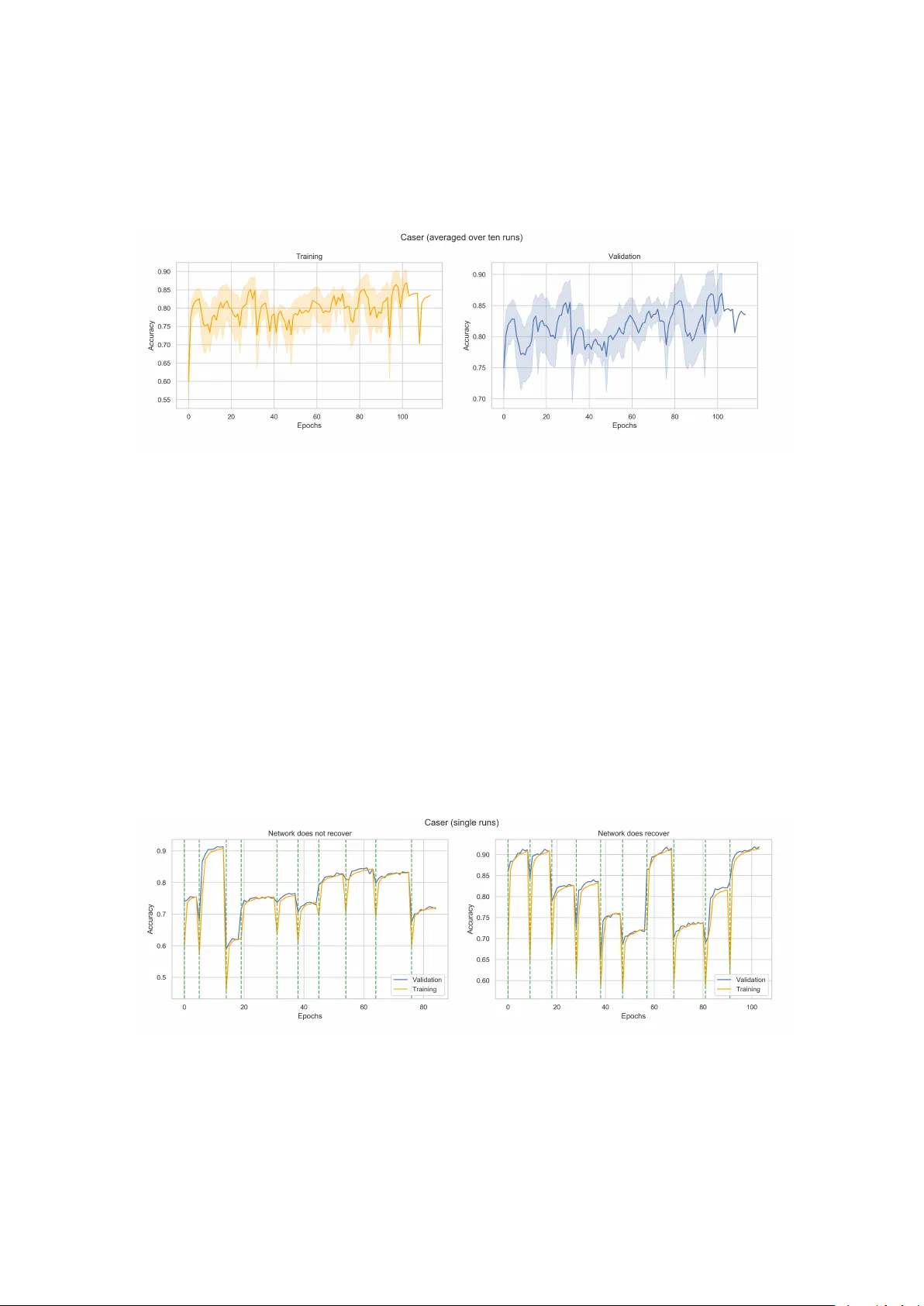
Automated Arc hitecture Design for Deep Neural Net w orks b y Steven Abreu Ja cobs University Bremen Bac helor Thesis in Computer Science Prof. Herbert Jaeger Bac helor Thesis Sup ervisor Date of Submission: Ma y 17th, 2019 Jacobs Univ ersit y — F o cus Area Mobility With m y signature, I certify that this thesis has b een written b y me using only the in- dicated resources and materials. Where I hav e presented data and results, the data and results are complete, genuine, and ha ve been obtained by me unless otherwise ackno wl- edged; where my results derive from computer programs, these computer programs ha ve b een written b y me unless otherwise ac knowledged. I further conﬁrm that this thesis has not b een submitted, either in part or as a whole, for any other academic degree at this or another institution. Signature Place, Date Abstract Mac hine learning has made tremendous progress in recen t y ears and received large amounts of public atten tion. Though we are still far from designing a full artiﬁcially intelligen t agen t, mac hine learning has brought us many applications in whic h computers solve h uman learning tasks remark ably well. Muc h of this progress comes from a recen t trend within mac hine learning, called de ep le arning . Deep learning mo dels are resp onsible for many state-of-the-art applications of machine learning. Despite their success, deep learning mo dels are hard to train, very diﬃcult to understand, and often times so complex that training is only p ossible on v ery large GPU clusters. Lots of work has been done on enabling neural net works to learn eﬃciently . Ho wev er, the design and arc hitecture of suc h neural netw orks is often done manually through trial and error and exp ert kno wledge. This thesis insp ects diﬀerent approaches, existing and no vel, to automate the design of deep feedforward neural net w orks in an attempt to create less complex mo dels with go o d p erformance that take aw ay the burden of deciding on an arc hitecture and mak e it more eﬃcient to design and train such deep netw orks. iii Con tents 1 Motiv ation 1 1.1 Relev ance of Machine Learning . . . . . . . . . . . . . . . . . . . . . . . . . 1 1.2 Relev ance of Deep Learning . . . . . . . . . . . . . . . . . . . . . . . . . . . 1 1.2.1 Ineﬃciencies of Deep Learning . . . . . . . . . . . . . . . . . . . . . 1 1.3 Neural Ne t work Design . . . . . . . . . . . . . . . . . . . . . . . . . . . . . . 2 2 In tro duction 3 2.1 Sup ervised Mac hine Learning . . . . . . . . . . . . . . . . . . . . . . . . . . 3 2.2 Deep Learning . . . . . . . . . . . . . . . . . . . . . . . . . . . . . . . . . . 3 2.2.1 Artiﬁcial Neural Netw orks . . . . . . . . . . . . . . . . . . . . . . . . 4 2.2.2 F eedforward Neural Net works . . . . . . . . . . . . . . . . . . . . . . 4 2.2.3 Neural Net w orks as Univ ersal F unction Approximators . . . . . . . . 4 2.2.4 Relev ance of Depth in Neural Netw orks . . . . . . . . . . . . . . . . 6 2.2.5 Adv an tages of Deep er Neural Netw orks . . . . . . . . . . . . . . . . 7 2.2.6 The Learning Problem in Neural Net works . . . . . . . . . . . . . . 8 3 Automated Architecture Design 9 3.1 Neural Architecture Search . . . . . . . . . . . . . . . . . . . . . . . . . . . 9 3.1.1 Non-Adaptiv e Searc h - Grid and Random Search . . . . . . . . . . . 10 3.1.2 Adaptiv e Searc h - Ev olutionary Searc h . . . . . . . . . . . . . . . . . 10 3.2 Dynamic Learning . . . . . . . . . . . . . . . . . . . . . . . . . . . . . . . . 11 3.2.1 Regularization Methods . . . . . . . . . . . . . . . . . . . . . . . . . 11 3.2.2 Destructiv e Dynamic Learning . . . . . . . . . . . . . . . . . . . . . 12 3.2.3 Constructiv e Dynamic Learning . . . . . . . . . . . . . . . . . . . . . 14 3.2.4 Com bined Destructiv e and Constructiv e Dynamic Learning . . . . . 17 3.3 Summary . . . . . . . . . . . . . . . . . . . . . . . . . . . . . . . . . . . . . 17 4 Empirical Findings 19 4.1 Outline of the Inv estigation . . . . . . . . . . . . . . . . . . . . . . . . . . . 19 4.1.1 In vestigated T echniques for Automated Arc hitecture Design . . . . . 19 4.1.2 Benc hmark Learning T ask . . . . . . . . . . . . . . . . . . . . . . . . 20 4.1.3 Ev aluation Metrics . . . . . . . . . . . . . . . . . . . . . . . . . . . . 20 4.1.4 Implemen tation Details . . . . . . . . . . . . . . . . . . . . . . . . . 21 4.2 Searc h Algorithms . . . . . . . . . . . . . . . . . . . . . . . . . . . . . . . . 21 4.2.1 Man ual Searc h . . . . . . . . . . . . . . . . . . . . . . . . . . . . . . 22 4.2.2 Random Searc h . . . . . . . . . . . . . . . . . . . . . . . . . . . . . . 23 4.2.3 Ev olutionary Searc h . . . . . . . . . . . . . . . . . . . . . . . . . . . 24 4.2.4 Conclusion . . . . . . . . . . . . . . . . . . . . . . . . . . . . . . . . 27 4.3 Constructiv e Dynamic Learning Algorithm . . . . . . . . . . . . . . . . . . 30 4.3.1 Cascade-Correlation Net w orks . . . . . . . . . . . . . . . . . . . . . 30 4.3.2 F orward Thinking . . . . . . . . . . . . . . . . . . . . . . . . . . . . 38 4.3.3 Automated F orward Thinking . . . . . . . . . . . . . . . . . . . . . . 40 4.3.4 Conclusion . . . . . . . . . . . . . . . . . . . . . . . . . . . . . . . . 42 4.4 Conclusion . . . . . . . . . . . . . . . . . . . . . . . . . . . . . . . . . . . . 43 5 F uture W ork 45 iv 1 Motiv ation 1.1 Relev ance of Machine Learning Mac hine Learning has made tremendous progress in recen t years. Although we are not able to replicate human-lik e in telligence with current state-of-the-art systems, machine learning systems ha ve outp erformed humans in some domains. One of the ﬁrst imp ortant milestones has b een achiev ed when DeepBlue defeated the world champion Garry Kasparo v in a game of c hess in 1997. Machine learning research has b een highly activ e since then and pushed the state-of-the-art in domains like image classiﬁcation, text classiﬁcation, lo calization, question answering, natural language translation and rob otics further. 1.2 Relev ance of Deep Learning Man y of today’s state-of-the-art systems are p ow ered b y deep neural netw orks (see Section 2.2). AlphaZero’s deep neural netw ork coupled with a reinforcement learning algorithm b eat the world champion in Go - a game that was previously b elieved to b e to o complex to b e play ed comp etitively b y a machine [Silv er et al., 2018]. Deep learning has also b een applied to conv olutional neural net w orks - a sp ecial kind of neural net work architecture that was initially prop osed by Y ann LeCun [LeCun and Bengio, 1998]. One of these deep con volutional neural net works, using ﬁve lay ers, has b een used to achiev e state-of-the-art p erformance in image classiﬁcation [Krizhevsky et al., 2017]. Overfeat, an eight la yer deep conv olutional neural net work, has b een trained on image lo calization, classiﬁcation and detection with very comp etitive results [Sermanet et al., 2013]. Another remark ably complex CNN has b een trained with 29 con volutional la yers to b eat the state of the art in sev eral text classiﬁcation tasks [Conneau et al., 2016]. Ev en a complex task that requires co ordination b etw een vision and control, such as screwing a cap on a b ottle, has been solved comp etitiv ely using suc h deep arc hitectures. Levine et al. [2016] used a deep con volutional neural netw ork to represen t p olicies to solve such rob otic tasks. Recurrent netw orks are particularly p opular in time series domains. Deep recurrent net works hav e b een trained to ac hieve state-of-the-art performance in generating captions for given images [Vin y als et al., 2015]. Go ogle uses a Long Short T erm Memory (LSTM) net work to achiev e state- of-the-art p erformance in machine translation [W u et al., 2016]. Other deep net work arc hitectures ha ve b een prop osed and successfully achiev ed state-of-the-art p erformance, suc h as dynamic memory net works for natural language question answering [Kumar et al., 2016]. 1.2.1 Ineﬃciencies of Deep Learning Eviden tly , deep neural netw orks are currently pow ering man y , if not most, state-of-the-art mac hine learning systems. Many of these deep learning systems train mo del that are ric her than needed and use elab orate regularization techniques to keep the neural netw ork from o verﬁtting on the training data. Man y mo dern deep learning systems achiev e state-of-the-art p erformance using highly complex mo dels by inv esting large amounts of GPU p ow er and time as well as feeding the system very large amounts of data. This has b een made p ossible through the recent 1 explosion of computational p ow er as well as through the a v ailability of large amounts of data to train these systems. It can b e argued that deep learning is ineﬃcien t b ecause it trains bigger netw orks than needed for the function that one desires to learn. This comes at a high exp ense in the form of computing p ow er, time and the need for larger training datasets. 1.3 Neural Netw ork Design The goal of designing a neural net work is manifold. The primary goal is to minimize the neural netw ork’s exp ected loss for the learning task. Because the exp ected loss cannot alw ays b e computed in practice, this goal is often re-deﬁned to minimizing the loss on a set of unseen test data. Aside from maximizing p erformance, it is also desirable to minimize the resources needed to train this net w ork. I diﬀerentiate b etw een c omputational r esour c es (suc h as computing p o wer, time and space) and human r esour c es (suc h as time and eﬀort). In my opinion, the goal of minimizing human resources is often ov erlo oked. Many mo dels, esp ecially in deep learning, are designed through trial, error and exp ert knowledge. This man ual design process is rarely interpretable or repro ducible and as suc h, little formal kno wledge is gained ab out the working of neural netw orks - aside from having a neural net work design that may work well for a sp eciﬁc learning task. In order to a v oid the diﬃculties of deﬁning and assessing the amount of human resources needed for the neural net work design process, I am in tro ducing a new goal for the design of neural netw orks: level of automaticity . The lev el of automaticity in neural netw ork design is in versely prop ortional to the num b er of decision that need to b e made by a human in the neural netw ork design pro cess. When dealing with computational resources for neural netw orks, one migh t naturally fo cus on optimizing the amount of computational resources needed during the training pro cess. Ho wev er, the amount of resources needed for utilizing the neural net work in practice are also very imp ortant. A neural netw ork is commonly trained once and then used many times once it is trained. The computational resources needed for the utilization of the trained neural net work sums up and should b e considered when designing a neural net work. A go o d measure is to reduce the mo del complexity or net work size. This goal reduces the computational resources needed for the neural netw ork in practice while sim ultaneously acting as a regularizer to incentivize neural netw orks to b e smaller - hence prefering simpler mo dels o ver more complex ones, as Occam’s razor states. T o conclude, the goal of designing a neural netw ork is to maximize p erformanc e (usually b y minimizing a chosen loss function on unseen test data), minimize c omputational r e- sour c es (during training), maximize the level of automaticity (b y minimizing the amount of decisions that need to b e made b y a h uman in the design pro cess), and to minimize the mo del’s c omplexity (e.g. b y minimizing the net work’s size). 2 2 In tro duction 2.1 Sup ervised Machine Learning In this pap er, I will be fo cusing on sup ervise d machine le arning . In sup ervised mac hine learning, one tries to estimate a function f : E X 7→ E Y where t ypically E X ⊆ R m and E Y ⊆ R n , given training data in the form of ( x i , y i ) i =1 ,..,N , with y i ≈ f ( x i ). This training data represen ts existing input-output pairs of the function that is to b e estimated. A machine learning algorithm takes the training data as input and outputs a function estimate f est with f est ≈ f . The goal of the sup ervised mac hine learning task is to minimize a loss function L : L : E Y × E Y 7→ R ≥ 0 In order to assess a function estimate’s accuracy , it should alwa ys b e assessed on a set of unseen input-output pairs. This is due to overﬁtting , a common phenomenon in machine learning in whic h a machine learning mo del memorizes part of the training data which leads to go o d p erformance on the training set and (often) bad generalization to unseen patterns. One of the biggest challenges in mac hine learning is to generalize well. It is trivial to memorize training data and correctly classifying these memorized samples. The c hallenge lies in correctly classifying previously unseen samples, based on what was seen in the training dataset. A supervised machine learning problem is speciﬁed by lab eled training data ( x i , y i ) i =1 ,..,N with x i ∈ E X , y i ∈ E Y and a loss function which is to b e minimized. Often times, the loss function is not part of the problem statement and instead needs to b e deﬁned as part of solving the problem. Giv en training data and the loss function, one needs to decide on a candidate set C of functions that will b e considered when estimating the function f . The learning algorithm L is an eﬀective procedure to choose one or more particular func- tions as an estimate for the given function estimation task, minimizing the loss function in some wa y: L ( C , L, ( x i , y i ) i =1 ,..N ) ∈ C T o summarize, a sup ervised learning problem is giv en b y a set of lab eled data points ( x i , y i ) i =1 ,..N whic h one typically calls the training data. The loss function L gives us a measure for how go o d a prediction is compared to the true target v alue and it can b e included in the problem statement. The sup ervised learning task is to ﬁrst decide on a candidate set C of functions that will b e considered. Finally , the learning algorithm L giv es an eﬀective pro cedure to choose one function estimate as the solution to the learning problem. 2.2 Deep Learning Deep learning is a subﬁeld of machine learning that deals with de ep artiﬁcial neur al net- works . These artiﬁcial neur al networks (ANNs) can represent arbitrarily complex func- tions (see section 2.2.3). 3 2.2.1 Artiﬁcial Neural Netw orks An artiﬁcial neural netw ork (ANN) (or simply , neural netw ork) consists of a set V of v = | V | pro cessing units, or neurons. Each neuron p erforms a transfer function of the form y i = f i   n X j =1 w ij x j − θ i   where y i is the output of the neuron, f i is the activ ation function (usually a nonlinear function suc h as the sigmoid function), x j is the output of neuron j , w ij is the connection w eight from node j to no de i and θ i is the bias (or threshold) of the no de. Input units are constan t, reﬂecting the function input v alues. Output units do not forward their output to an y other neurons. Units that are neither input nor output units are called hidden units. The en tire netw ork can b e described b y a directed graph G = ( V , E ) where the directed edges E are giv en through a weigh t matrix W ∈ R v × v . An y non-zero entry in the weigh t matrix at index ( i, j ), i.e. w ij 6 = 0 denotes that there is a connection from neuron j to neuron i . A neural netw ork is deﬁned by its ar chite ctur e , a term that is used in diﬀerent wa ys. In this pap er, the architecture of a neural net work will alwa ys refer to the net work’s no de connectivit y pattern and the no des’ activ ation functions. ANN’s can b e segmen ted in to feedforward and recurrent netw orks based on their netw ork top ology . An ANN is feedforward if there exists an ordering of neurons such that every neuron is only connected to a neuron further down the ordering. If such an ordering do es not exist, then the net work is recurrent. In this thesis, I will only b e considering feedforw ard neural net w orks. 2.2.2 F eedforw ard Neural Netw orks A feedforw ard netw ork can be visualized as a la yered net work, with la yers L 0 through L K . The la y er L 0 is called the input lay er and L K is called the output lay er. Intermediate la yers are called hidden lay ers. One can think of the lay ers as subsequen t feature extractors: the ﬁrst hidden lay er L 1 is a feature extractor on the input unit. The second hidden lay er L 2 is a feature extractor on the ﬁrst hidden lay er - th us a second order feature extractor on the input. The hidden la yers can compute increasingly complex features on the input. 2.2.3 Neural Net works as Univ ersal F unction Approximators A classical universal appro ximation theorem states that standard feedforw ard neural net- w orks with only one hidden lay er using a squashing activ ation function (a function Ψ : R 7→ [0 , 1] is a squashing function, according to Hornik et al. [1989], if it is non-decreasing, Ψ λ →∞ ( λ ) = 1 and Ψ λ →−∞ ( λ ) = 0) can b e used to approximate any con tinuous function on c omp act subsets of R n with an y desired non-zero amoun t of error [Hornik et al., 1989]. The only requirement is that the net work m ust ha ve suﬃciently many units in its hidden la yer. 4 A simple example can demonstrate this univ ersal appro ximation theorem for neural net- w orks. Consider the binary classiﬁcation problem in Figure 1 of the kind f : [0 , 1] 2 → { 0 , 1 } . The function solving this classiﬁcation problem can b e represented using an MLP . As stated by the universal approximation theorem, one can approximate this function to arbitrary precision using an MLP with one hidden lay er. Figure 1: Binary classiﬁcation problem. Y ello w area is one class, ev erything else is the other class. Right is the shallo w neural net work that should represent the classiﬁcation function. Figure taken from Bhiksha Ra j’s lecture slides in CMU’s ’11-785 Introduction to Deep Learning’. The diﬃcult y in represen ting the desired classiﬁcation function is that the classiﬁcation is split in to tw o separate, disconnected decision regions. Represen ting either one of these shap es is trivial. One can add one neuron p er side of the p olygon which acts as a feature detector to detect the decision b oundary represen ted b y this side of the p olygon. One can then add a bias in to the hidden lay er with a v alue of b h = − N ( N is the num b er of sides of the p olygon), use a relu-activ ated output unit and one has built a simple neural net work whic h returns 1 iﬀ all hidden neurons ﬁre, i.e. when the p oint lies within the b oundary of ev ery side of the p olygon, i.e. when the p oint lies within the p olygon. (a) Decision b ound- ary for a square (b) Decision bound- ary for a hexagon (c) Decision plot for a square (d) Decision plot for a hexagon Figure 2: Decision plots and boundaries for simple binary classiﬁcation problems. Figures tak en from Bhiksha Ra j’s lecture slides in CMU’s ’11-785 In tro duction to Deep Learning’. This approac h generalizes neither to shap es that are not conv ex nor to multiple, discon- nected shap es. In order to appro ximate any decision b oundary using just one hidden la yer, one can use an n -sided p olygon. Figure 2a and 2b sho w the decision boundaries for a square and a hexagon. A problem arises when the t wo shapes are close to each other; the areas outside the b oundaries add up to v alues larger or equal to those within the b ound- aries of eac h shap e. In the plots of Figure 2c and 2d, one can see that the b oundaries of 5 the decision regions don’t fall oﬀ quickly enough and will add up to large v alues, if there are tw o or more such shap es in close pro ximit y . Figure 3: Decision plot and corresp onding MLP structure for approximating a circle. Figure tak en from Bhiksha Ra j’s lecture slides in CMU’s ’11-785 In tro duction to Deep Learning’. Ho wev er, as one increases the sides n of the polygon, the b oundaries will fall oﬀ more quic kly . In the limit of n → ∞ , the shap e b ecomes a near p erfect cylinder, with v alue n for the area within the cylinder and n/ 2 outside. Using a bias unit of b h = − n/ 2, one can turn this into a near-circular shap e with v alue n/ 2 in the shap e and v alue 0 everywhere else, as shown in Figure 3. One can no w add multiple near-circles together in the same la yer of the neural net w ork. Given this setup, one can now comp ose an arbitrary ﬁgure by ﬁtting it with an arbitrary n umber of near-circles. The smaller these near-circles, the more accurate this classiﬁcation problem can b e represen ted by a netw ork. With this setup, it is p ossible to capture any decision b oundary . This pro cedure to build a neural net work with one hidden lay er to build a classiﬁer for arbitrary ﬁgures has a problem: the num b er of hidden units needed to represent this function b ecome arbitrarily high. In this pro cedure, I hav e set n , the num b er of hidden units to represent a circle to be v ery large and I am using man y of these circles to represen t the entire function. This will result in a v ery ( very ) large num b er of units in the hidden la yer. This is a general phenomenon: ev en though a netw ork with just one hidden la y er can rep- resen t any function (with some restrictions, see ab o ve) to arbitrary precision, the num b er of units in this hidden lay er often b ecomes intractably large. Learning algorithms often fail to learn complicated functions correctly without o verﬁtting the training data in such ”shallo w” net works. 2.2.4 Relev ance of Depth in Neural Net w orks The classiﬁcation function from Figure 1 can be built using a smaller net work, if one allows for multiple hidden lay ers. The ﬁrst lay er is a feature detector for every p olygon’s edge. The second la yer will act as an AND gate for every distinct p olygon - detecting all those p oin ts that lie within all the p olygon’s edges. The output la yer will then act as an OR gate for all neurons in the second la yer, th us detecting all p oints that lie in any of the p olygons. With this, one can build a simple netw ork that p erfectly represents the desired classiﬁcation function. The net w ork and decision b oundaries are shown in Figure 4. 6 Figure 4: Decision b oundary and corresp onding t wo-la y er classiﬁcation netw ork. Figure tak en from Bhiksha Ra j’s lecture slides in CMU’s ’11-785 In tro duction to Deep Learning’. By adding just one additional lay er into the netw ork, the n umber of hidden neurons has b een reduced from n shallow → ∞ to n deep = 12. This shows how the depth of a net work can increase the resulting mo del capacity faster than an increase in the n um b er of units in the ﬁrst hidden lay er. 2.2.5 Adv an tages of Deep er Neural Net works It is diﬃcult to understand how the depth of an arbitrary neural net w ork inﬂuences what kind of functions the netw ork can compute and how well these netw orks can b e trained. Early researc h has fo cused on shallow netw orks and their conclusions cannot b e generalized to deep er arc hitectures, such as the universal approximation theorem for net works with one hidden lay er [Hornik et al., 1989] or an analysis of a neural netw ork’s expressivity based on an analogy to b o olean circuits b y Maass et al. [1994]. Sev eral measures ha ve b een prop osed to formalize the notion of mo del capacit y and the complexit y of functions which a statistical learning algorithm can represen t. One of the most famous such formalization is that of the V apnik Chervonenkis dimension (VC di- mension) [V apnik and Chervonenkis, 2015]. Recen t pap ers hav e fo cused on understanding the b eneﬁts of depth in neural net works. The V C dimension as a measure of capacit y has b een applied to feedforw ard neural net work with piecewise p olynomial activ ation functions, suc h as relu, to prov e that a net work’s mo del capacit y gro ws b y a factor of W log W with depth compared to a similar growth in width [Bartlett et al., 1999]. There are examples of functions that a deep er netw ork can express and a more shallow net work cannot appro ximate unless the width is exp onen tial in the dimension of the input ([Eldan and Shamir, 2016] and [T elgarsky, 2015]). Upp er and low er b ounds ha ve b een established on the net work complexit y for diﬀeren t n umbers of hidden units and activ ation functions. These sho w that deep architectures can, with the same num b er of hidden units, realize maps of higher complexit y than shallow architectures [Bianc hini and Scarselli, 2014]. Ho wev er, the aforementioned pap ers either do not take in to account the depth of mo dern deep learning models or only presen t ﬁndings for speciﬁc c hoices of w eights of a deep neural netw ork. 7 Using Riemannian geometry and dynamical mean ﬁeld theory , P o ole et al. [2016] sho w that generic deep neural net works can ”eﬃciently compute highly expressiv e functions in w ays that shallo w netw orks cannot” whic h ”quan tiﬁes and demonstrates the pow er of deep neural netw orks to disentangle curved input manifolds” [P o ole et al., 2016]. Ragh u et al. [2017] introduced the notion of a tr aje ctory ; given t wo points in the input space x 0 , x 1 ∈ R m , the tra jectory x ( t ) is a curve parametrized by t ∈ [0 , 1] with x (0) = x 0 and x (1) = x 1 . They argue that the tra jectory’s length serv es as a measure of net work expressivit y . By measuring the tra jectory lengths of the input as it is transformed b y the neural net w ork, they found that the netw ork’s depth increases complexit y (giv en by the tra jectory length) of the computed function exponentially , compared to the net work’s width. 2.2.6 The Learning Problem in Neural Net w orks A net work architecture b eing able to appr oximate any function do es not alw ays mean that a netw ork of that architecture is able to le arn any function. Whether or not neural net work of a ﬁxed architecture can b e trained to represent a giv en function depends on the learning algorithm used. The learning algorithm needs to ﬁnd a set of parameters for which the neural netw ork computes the desired function. Giv en a function, there exists a neural net work to represen t this function. But ev en if suc h an architecture is given, there is no universal algorithm whic h, given training data, ﬁnds the correct set of parameters for this netw ork such that it will also generalize well to unseen data p oints [Go o dfellow et al., 2016]. Finding the optimal neural netw ork architecture for a given learning task is an unsolv ed problem as well. Zhang et al. [2016] argue that most deep learning systems are built on mo dels that are rich enough to memorize the training data. Hence, in order for a neural net work to learn a function from data, it has to learn the net- w ork architecture and the parameters of the neural netw ork (connection weigh ts). This is commonly done in sequence but it is also possible to do both sim ultaneously or iteratively . 8 3 Automated Arc hitecture Design Cho osing a ﬁtting arc hitecture is a big challenge in deep learning. Choosing an unsuitable arc hitecture can make it imp ossible to learn the desired function. Choosing an optimal arc hitecture for a learning task is an unsolved problem. Currently , most deep learning systems are designed by exp erts and the design relies on h yp erparameter optimization through a combination of grid searc h and manual searc h [Bergstra and Bengio, 2012] (see Laro c helle et al. [2007], LeCun et al. [2012], and Hinton [2012]). This man ual design is tedious, computationally exp ensiv e, and architecture decisions based on exp erience and in tuition are very diﬃcult to formalize and thus, reuse. Man y algorithms ha ve b een prop osed for the architecture design of neural netw orks, with v arying lev els of automaticit y . In this thesis, I will b e referring to these algorithms as automate d ar chite ctur e design algorithms . Automated architecture algorithms can b e broadly segmen ted into neural netw ork arc hi- tecture search algorithms (also called neural architecture searc h, or NAS) and dynamic learning algorithms, b oth of which are discussed in this section. 3.1 Neural Architecture Searc h Neural architecture search is a natural c hoice for the design of neural netw orks. NAS metho ds are already outp erforming man ually designed arc hitectures in image classiﬁcation and ob ject detection ([Zoph et al., 2018] and [Real et al., 2018]). Elsk en et al. [2019] prop ose to categorize NAS algorithms according to three dimensions: searc h space, search strategy , and p erformance estimation strategy . The authors describ e these as follows. The search space deﬁnes the set of arc hitectures that are considered by the searc h algorithm. Prior knowledge can b e incorp orated in to the searc h space, though this ma y limit the exploration of no v el architectures. The search strategy deﬁnes the searc h algorithm that is used to explore the searc h space. The searc h algorithm deﬁnes ho w the exploration-exploitation tradeoﬀ is handled. The performance estimation strategy deﬁnes ho w the p erformance of a neural net work arc hitecture is assessed. Naiv ely , one ma y train a neural netw ork architecture but this is ob ject to random ﬂuctuations due to initial random weigh t initializations, and obviously very computationally exp ensiv e. In this thesis, I will not b e considering the searc h space part of the NAS algorithms. Instead, I will k eep the searc h space constant across all NAS algorithms. I will not go in depth ab out the p erformance estimation strategy in the algorithms either, instead using one constan t form of constant estimation - training a net work architecture once for the same num b er of ep o c hs (dep ending on time constraints). Man y search algorithms can b e used in NAS algorithms. Elsken et al. [2019] names random searc h, Ba yesian optimization, evolutionary methods, reinforcemen t learning, and gradien t-based methods. Search algorithms can b e divided in to adaptiv e and non-adaptive algorithms, where adaptive search algorithms adapt future searches based on the p erfor- mance of already tested instances. In this thesis, I will only consider grid search and random searc h as non-adaptiv e searc h algorithms, and ev olutionary searc h as an adaptive searc h algorithm. F or the following discussion, let A b e the set of all p ossible neural netw ork arc hitectures 9 and A 0 ⊆ A b e the search space deﬁned for the NAS algorithm - a subset of all p ossible arc hitectures. 3.1.1 Non-Adaptiv e Searc h - Grid and Random Search The simplest w ay to automatically design a neural netw ork’s arc hitecture ma y be to simply try diﬀerent architectures from a deﬁned subset of all p ossible neural netw ork arc hitec- tures and c ho ose the one that p erforms the best. One chooses elemen ts a i ∈ A 0 , tests these individual architectures and chooses the one that p erforms the b est. The p erformance is usually measured through ev aluation on an unseen testing set or through a cross v alida- tion pro cedure - a tec hnique which artiﬁcially splits the training data into training and v alidation data and uses the unseen v alidation data to ev aluate the mo del’s p erformance. The tw o most widely kno wn search algorithms that are frequently used for hyperparame- ter optimization (whic h includes architecture search) are grid se ar ch and r andom se ar ch . Naiv e grid search p erforms an exhaustive, enumerated search within the chosen subset A 0 of p ossible architectures - where one needs to also sp ecify some kind of step size, a discretization scheme whic h determines ho w ”ﬁne” the searc h within the architecture sub- space should b e. Adaptive grid searc h algorithms use adaptiv e grid sizes and are not exhaustiv e. Random search do es not need a discretization scheme, it chooses elements from A 0 at random in each iteration. Both grid and random search are non-adaptiv e algo- rithms: they do not v ary the course of the exp erimen t by considering the p erformance of already tested instances [Bergstra and Bengio, 2012]. Laro chelle et al. [2007] ﬁnds that, in the case of a 32-dimensional searc h problem of deep b elief netw ork optimization, random searc h was not as go o d as the sequential combination of manual and grid searc h from an exp ert b ecause the eﬃciency of sequential optimization o v ercame the ineﬃciency of the grid searc h emplo yed at ev ery step [Bergstra and Bengio, 2012]. Bergstra and Bengio [2012] concludes that sequen tial, adaptive algorithms should b e considered in future w ork and random search should b e used as a p erformance baseline. 3.1.2 Adaptiv e Searc h - Ev olutionary Searc h In the past three decades, lots of research has b een done on genetic algorithms and artiﬁcial neural net works. The tw o areas of research hav e also b een combined and I shall refer to this com bination as evolving artiﬁcial neural netw orks (EANN), based on a literature review b y Y ao [1999]. Ev olutionary algorithms hav e b een applied to artiﬁcial neural net works to ev olve connection w eights, arc hitectures, learning rules, or any com bination of these three. These EANN’s can b e viewed as an adaptive system that is able to learn from data as w ell as ev olv e (adapt) its arc hitecture and learning rules - without h uman in teraction. Ev olutionary algorithms are p opulation based search algorithms whic h are deriv ed from the principles of natural ev olution. They are very useful in complex domains with man y lo cal optima, as is the case in learning the parameters of a neural net work [Choromansk a et al., 2015]. They do not require gradien t information which can b e a computational adv antage as the gradients for neural net work w eights can b e quite exp ensiv e to compute, esp ecially so in deep netw orks and recurrent net works. The sim ultaneous ev olution of connection w eights and netw ork architecture can be seen as a fully automated ANN design. The ev olution of learning rules can b e seen as a wa y of ”learning ho w to learn”. In this pap er, 10 I will b e fo cusing on the ev olution of neural net work arc hitectures, staying indep enden t of the algorithm that is used to optimize connection weigh ts. The t wo key issues in the design of an ev olutionary algorithm are the representation and the search op erators. The architecture of a neural netw ork is deﬁned by its no des, their connectivit y and e ac h node’s transfer function. The architecture can b e enco ded as a string in a multitude of w ays, whic h will not b e discussed in detail here. A general cycle for the ev olution of net work architectures has been proposed b y Y ao [1999]: 1. Deco de eac h individual in the current generation in to an arc hitecture. 2. T rain each ANN in the same wa y , using n distinct random initializations. 3. Compute the ﬁtness of each arc hitecture according to the av eraged training results. 4. Select paren ts from the p opulation based on their ﬁtness. 5. Apply searc h op erators to paren ts and generate oﬀspring to form the next generation. It is apparent that the p erformance of an EANN dep ends on the enco ding scheme of the arc hitecture, the deﬁnition of the ﬁtness function, and the search op erators applied to the parents to generate oﬀspring. There will b e some residual noise in the pro cess due to the sto c hastic nature of ANN training. Hence, one should view the computed ﬁtness as a heuristic v alue, an approximation, for the true ﬁtness v alue of an architecture. The larger the num b er n of diﬀerent random initializations that are run for each arc hitecture, the more accurate training results (and thus, the ﬁtness computation) b ecomes. How ever, increasing n leads to a large increase in time needed for each iteration of the evolutionary algorithm. 3.2 Dynamic Learning Dynamic learning algorithms in neural netw orks are algorithms that mo dify a neural net work’s hyperparameters and top ology (here, I fo cus on the net w ork architecture) dy- namically as part of the learning algorithm, during training. These approac hes presen t the opp ortunit y to develop optimal net work arc hitectures that generalize well [W augh, 1994]. The netw ork architecture can b e mo diﬁed during training by adding complexit y to the net work or b y remo ving complexit y from the netw ork. The former is called a constructive algorithm, the latter a destructiv e algorithm. Naturally , the t wo can b e combined into an algorithm that can increase and decrease the netw ork’s complexit y as needed, in so-called com bined dynamic learning algorithms. These changes can aﬀect the no des, connections or w eigh ts of the net work - a go o d ov erview of possible netw ork changes is given by W augh [1994], see Figure 5. 3.2.1 Regularization Metho ds Before moving on to dynamic learning algorithms, it is necessary to clear up the clas- siﬁcation of these dynamic learning algorithms and clarify some underlying terminology . The set of destructiv e dynamic learning algorithms in tersects with the set of so-called regularization metho ds in neural net works. The origin of this confusion is the deﬁnition of dynamic learning algorithms. W augh [1994] deﬁnes dynamic learning algorithms to c hange either the no des, connections, or weights of the neural netw ork. If we contin ue 11 Figure 5: P ossible net work top ology c hanges, taken from W augh [1994] with this deﬁnition, w e will include all algorithms that reduce the v alues of connections w eights in the set of destructive dynamic learning, whic h includes regularization metho ds. Regularization metho ds p enalize higher connection weigh ts in the loss function (as a re- sult, connection weigh ts are reduced in v alue). Regularization is based on Occam’s razor whic h states that the simplest explanation is more likely to b e correct than more com- plex explanations. Regularization p enalizes suc h complex explanations (by reducing the connection weigh ts’ v alues) in order to simplify the resulting mo del. Regularization methods include w eight decay , in whic h a term is added to the loss function whic h p enalizes large w eigh ts, and drop out, whic h is explained in Section 3.2.2. F or completeness, I will co ver these tec hniques as instances of dynamic learning, how e v er I will not run any experiments on these regularization metho ds as the goal of this thesis is to insp ect metho ds to automate the ar chite ctur e design, for which the modiﬁcation of connection weigh ts is not relev ant. 3.2.2 Destructiv e Dynamic Learning In destructive dynamic learning, one starts with a net work arc hitecture that is larger than needed and reduces complexit y in the netw ork b y remo ving nodes, connections or reducing existing connection weigh ts. A key c hallenge in this destructive approach is the c hoice of starting netw ork. As opp osed to a minimal net work - which could simply b e a netw ork without any hidden units - it is diﬃcult to deﬁne a ”maximal” net work b ecause there is no upp er b ound on the netw ork size [W augh, 1994]. A simple solution would b e to choose a fully connected netw ork with K lay ers, where K is dep enden t on the learning task. An imp ortan t downside to the use of destructiv e algorithms is the computational cost. Starting with a v ery large netw ork and then cutting it down in size leads to man y redundant computations on the large netw ork. Most approac hes to destructiv e dynamic learning that mo dify the no des and connections (rather than just the connection w eights) are concerned with the pruning of hidden no des. The general approach is to train a netw ork that is larger than needed an d prune parts of the net work that are not essential. Reed [1993] suggests that most pruning algorithms can b e 12 divided into tw o groups; algorithms that estimate the sensitivity of the loss function with resp ect to the remo v al of an element and then remo ves those elements with the smallest eﬀect on the loss function, and those that add terms to the ob jective f unction that rew ards the netw ork for choosing the most eﬃcien t solution - s uc h as w eight deca y . I shall refer to those tw o groups of algorithms as sensitivit y calculation metho ds and penalty-term metho ds, resp ectiv ely - as prop osed by W augh [1994]. Other algorithms hav e b een proposed but will not b e included in this thesis for brevit y reasons (most notably , principal comp onen ts pruning [Levin et al., 1994] and soft weigh t- sharing as a more complex P enalty-T erm metho d [Nowlan and Hin ton, 1992]). Drop out This section follows Sriv asta v a et al. [2014]. Dropout refers to a wa y of regularizing a neural net work by randomly ”dropping out” en tire no des with a certain probability p in eac h la yer of the netw ork. At the end of training, each no de’s outgoing weigh ts are then m ultiplied with its probabilit y p of being dropp ed out. As the net works connection w eights are multiplied with a certain probability v alue p , where p ∈ [0 , 1], one can consider this tec hnique a kind of connection weigh t pruning and thus, in the following, I will consider drop out to b e a destructive algorithm. In tuitively , drop out drives hidden units in a net w ork to w ork with diﬀerent combinations of other hidden units, essentially driving the units to build useful features without relying on other units. Drop out can b e interpreted as a sto c hastic regularization tec hnique that w orks b y in tro ducing noise to its units. One can also view this ”dropping out” in a diﬀerent wa y . If the net work has n no des (excluding output notes), drop out can either include or not include this no de. This leads to a total of 2 n diﬀeren t net work conﬁgurations. At each step during training, one of these net work conﬁgurations is chosen and the weigh ts are optimized using some gradient descen t metho d. The en tire training can hence b e seen as training not just one net work but all p ossible 2 n net work arc hitectures. In order to get an ideal prediction from a ﬂexible-sized mo del such as a neural net work, one should av erage ov er the predictions of all p ossible settings of the parameters, w eighing each setting by its p osterior probabilit y giv en the training data. This pro cedure quic kly b ecomes intractable. In essence, drop out is a technique that can combine exp onen tially (exp onen tial in the num b er of no des) many diﬀeren t neural net w orks eﬃciently . Due to this mo del com bination, drop out is rep orted to tak e 2-3 times longer to train than a standard neural netw ork without drop out. This mak es drop out an eﬀectiv e algorithm that deals with a trade-oﬀ b et ween ov erﬁtting and training time. T o conclude, drop out can b e seen as b oth a regularization tec hnique and a form of mo del a veraging. It w orks remark ably well in practice. Sriv asta v a et al. [2014] rep ort large impro vemen ts across all architectures in an extensive empirical study . The ov erall arc hi- tecture is not c hanged, as the pruning happ ens only in terms of the magnitude of the connection weigh ts. P enalt y-T erm Pruning through W eigh t Deca y 13 W eight deca y is the b est-kno wn regularization technique that is frequently used in deep learning applications. It w orks by p enalizing net work complexity in the loss function, through some complexity measure that is added into the loss function - suc h as the n umber of free parameters or the magnitude of connection weigh ts. Krogh and Hertz [1992] show that w eight decay can impro ve generalization of a neural net work by suppressing irrelev an t comp onen ts of the weigh t vector and by suppressing some of the eﬀect of static noise on the targets. Sensitivit y Calculation Pruning Sietsma [1988] remov es no des whic h hav e little eﬀect on the o verall netw ork output and no des that are duplicated by other nodes. The author also discusses remo ving entire lay ers, if they are found to b e redundant [W augh, 1994]. Skeletonization is based on the same idea of the netw ork’s sensitivit y to no de remo v al and prop oses to remov e no des from the net work based on their relev ance during training [Mozer and Smolensky, 1989]. Optimal brain damage (OBD) uses second-deriv ativ e information to automatically delete parameters based on the ”saliency” of each param ter - reducing the num b er of parameters b y a factor of four and increasing its recognition accuracy slightly on a state-of-the-art net work [LeCun et al., 1990]. Optimal Brain Surgeon (OBS) enhances the OBD algorithm b y dropping the assumption that the Hessian matrix of the neural netw ork is diagonal (they rep ort that in most cases, the He ssian is actually strongly non-diagonal), and they rep ort ev en b etter results [Hassibi et al., 1993]. The algorithm was extended again by the same authors [Hassibi et al., 1994]. Ho wev er, metho ds based on sensitivity measures ha ve the disadv antage that they do not detect correlated elemen ts - suc h as t w o no des that cancel eac h other out and could be remo ved without aﬀecting the netw orks p erformance [Reed, 1993]. 3.2.3 Constructiv e Dynamic Learning In constructive dynamic learning, one starts with a minimal netw ork structure and itera- tiv ely adds complexity to the net work b y adding new no des or new connections to existing no des. Tw o algorithms for the dynamic construction of feed-forward neural net works are pre- sen ted in this section: the cascade-correlation algorithm (Cascor) and the forw ard thinking algorithm. Other algorithms ha v e b een prop osed but, for brevity , will not b e included in this pap er’s analysis (node splitting [Wynne-Jones, 1992], the tiling algorithm [Mezard and Nadal, 1989], the upstart algorithm [F rean, 1990], a pro cedure for determining the top ology for a three lay er neural netw ork [W ang et al., 1994], and meiosis netw orks that replace one ”o vertaxed” no de b y t wo no des [Hanson, 1990]). Cascade-correlation Netw orks 14 The cascade-correlation learning architecture (short: Cascor) was prop osed by F ahlman and Lebiere [1990]. It is a sup ervised learning algorithm for neural netw orks that contin- uously adds units in to the net work, trains them one by one and then freezes those unit’s input connections. This results in a net work that is not la yered but has a structure in whic h all input units are connected to all hidden units and the hidden units hav e a hierar- c hical ordering in whic h the one hidden unit’s output is fed into subsequen t hidden units as input. When training, Cascor k eeps a ”p o ol” of candidate units - p ossibly using diﬀerent nonlinear activ ation functions - and chooses the b est candidate unit. Figure 6 visualizes this architecture. So-called residual neural netw orks hav e b een very successful in tasks suc h as image recognition [He et al., 2016] through the use of similar skip connections. Cascor tak es the idea of skip connections and applies it to include netw ork connections from the input to every hidden no de in the netw ork. Figure 6: The cascade correlation neural net work architecture after adding tw o hidden units. Squared connections are frozen after training them once, crossed connections are retrained in eac h training iteration. Figure tak en and adapted from F ahlman and Lebiere [1990]. Cascor aims to solve tw o main problems that are found in the widely used backpropagation algorithm: the step-size pr oblem , and the moving tar get pr oblem . The step size problem o ccurs in gradient descen t optimization metho ds b ecause it is not clear how big the step in each parameter up date should b e. If the step size is to o small, the netw ork tak es to o long to conv erge to a lo cal minim um, if it is to o large, the learning algorithm will jump past lo cal minima and p ossibly not con verge to a go o d solution at all. Among the most successful wa ys of dealing with this step size problem are higher-order metho ds, which compute second deriv ativ es in order to get a goo d estimate of what the step size should b e (which is v ery exp ensive and often times in tractable), or some form of ”momen tum”, which k eeps trac k of earlier steps taken to mak e an educated guess ab out ho w large the step size should b e at the current step. The mo ving target problem o ccurs in most neural net works when all units are trained at the same time and cannot communicate with each other. This leads to all units trying to solv e the same learning task - which changes constantly . F ahlman and Lebiere prop ose an in teresting manifestation of the moving target problem which they call the ”herd eﬀect”. Giv en tw o sub-tasks, A and B, that must b e p erformed by the hidden units in a net work, eac h unit has to decide indep endently which of the t wo problems it will tackle. If task A generates a larger or more coherent error signal than task B, the hidden units will tend to 15 concen trate on A and ignore B. Once A is solved, the units will then see B as a remaining source of error. Units will mov e to wards task B and, in turn, problem A reapp ears. Cascor aims to solv e this moving target problem by only training one hidden unit at a time. Other approac hes, suc h as the forward thinking formulation, are less restricted and allo w the training of one entire la yer of units at a time [Hettinger et al., 2017]. In their original pap er, F ahlman and Lebiere rep orted go o d benchmark results on the t wo-spirals problem and the n-input parity problem. The main adv antages ov er net works using backpropagation were faster training (though this might also b e attributed to the use of the Quickprop learning algorithm), deep er netw orks without problems of v anishing gradien ts, p ossibilit y of incremen tal learning and, in the n-input parity problem, fewer hidden units in total. In the literature, Cascor has b een criticized for p o or p erformance on regression tasks due to an ov ercomp ensation of errors whic h comes from training on the error correlation rather than on the error signal directly ([Littmann and Ritter, 1992], [Prechelt, 1997]). Cascor has also b een criticized for the use of its cascading structure rather than adding each hidden unit into the same hidden la y er. Littmann and Ritter [1992] presen t a diﬀerent version of Cascor that is based on error minimization rather than error correlation maximization, called Caser. They also presen t another mo diﬁed v ersion of Cascor, called Casqef, whic h is trained on error minimization and uses additional non-linear functions on the output of cascaded units. Caser do esn’t do any b etter than Cascor, while Casqef outp erforms Cascor in more complicated tasks - lik ely b ecause of the additional nonlinearities in tro duced by the nonlinear functions on the cascaded units. Littmann and Ritter [1993] sho w that Cascor is fa vorable for ”extracting information from small data sets without running the risk of ov erﬁtting” when compared with shallo w broad arc hitectures that contain the same num b er of no des. How ev er, this comparison do es not tak e in to account deep la yered architectures that are p opular in today’s deep learning landscap e. Sjogaard [1991] suggests that the cascading of hidden units has no adv antage o ver the same algorithm adding each unit in to the same hidden lay er. Prec helt [1997] ﬁnds that Cascor’s cascading structure is sometimes b etter and sometimes w orse than adding all the units into one single hidden la yer - while in most cases it do esn’t mak e a signiﬁcant diﬀerence. They also ﬁnd that training on cov ariance is more suitable for classiﬁcation tasks while training on error minimization is more suitable for regression tasks. Y ang and Hona v ar [1998] ﬁnd that in their exp erimen ts, Cascor learns 1-2 orders of magni- tude faster than a netw ork trained with backpropagation, results in substantially smaller net works and only a minor degradation of accuracy on the test data. They also ﬁnd that Cascor has a large num b er of design parameters that need to b e set, which is usually done through exploratory runs whic h, in turn, translates in to increased computational costs. According to the authors, this might b e worth it ”if the goal is to ﬁnd relatively small net works that p erform the task w ell” but ”it can b e impractical in situations where fast learning is the primary goal”. Most of the literature av ailable for Cascor is ov er 20 years old. Cascor seems to not hav e b een activ ely in vestigated in recen t y ears. Through email corresp ondence with the original 16 pap er’s author, Scott E. F ahlman at CMU, and his PhD student Dean Alderucci, I was made aw are of the fact that research on Cascor has b een inactiv e for o v er tw en ty years. Ho wev er, Dean is curren tly w orking on establishing mathematical pro ofs inv olving how Cascor op erates, and adapting the recurren t v ersion of Cascor tosentence classiﬁers and p ossibly language modeling. With my exp eriments, I am starting a preliminary in v estiga- tion into whether Cascor is still a promising learning algorithm after t w o decades. F orw ard Thinking In 2017, Hettinger et al. [2017] proposed a general framew ork for a greedy training of neural netw orks one lay er at a time, which they call ”forw ard thinking”. They giv e a general mathematical description of the forw ard thinking framew ork, in whic h one la yer is added at a time, then trained on the desired output and ﬁnally added into the netw ork while freezing the lay er’s input w eights and discarding its output weigh ts. There are no skip connections, as in Cascor. The goal is to make the data ”more separable”, i.e. b etter b eha ved after eac h la yer. In their exp eriments, Hettinger et al. [2017] used a fully-connected neural netw ork with four hidden lay ers to compare training using forward thinking against traditional back- propagation. They report similar test accuracy and higher training accuracy with the forw ard thinking netw ork - which hints at o verﬁtting, th us more needs to b e done for regularization in the forward thinking framework. How ever, forward thinking w as signiﬁ- can tly faster. T raining with forward thinking was ab out 30% faster than backpropagation - ev en though they used libraries whic h w ere optimized for backpropagation. They also sho wed that a con v olutional netw ork trained with forw ard thinking outp erformed a net- w ork trained with bac kpropagation in training accuracy , testing accuracy while eac h epo ch to ok ab out 50% less time. In fact, the CNN trained using forw ard thinking achiev es near state-of-the-art p erformance after b eing trained for only 90 min utes on a single desktop mac hine. Both Cascor and forward thinking c onstruct neural net works in a greedy wa y , lay er b y la yer. Ho wev er, forward thinking trains la yers instead of individual units and while Cascor uses old data to train new units, forward thinking uses new, synthetic data to train a new la yer. 3.2.4 Com bined Destructiv e and Constructiv e Dynamic Learning As mentioned b efore, it is also p ossible to combine the destructive and constructive ap- proac h to dynamic learning. I was not able to ﬁnd any algorithms that ﬁt into this area, aside from W augh [1994], who prop osed a mo diﬁcation to Cascor which also prunes the net work. 3.3 Summary Man y curren t state-of-the-art machine learning solutions rely on deep neural net wor ks with arc hitectures muc h larger than necessary in order to solv e the task at hand. Through early stopping, drop out and other regularization tec hniques, these o verly large net works are preven ted from ov erﬁtting on the data. Finding a w ay to eﬃcien tly automate the 17 arc hitecture design of neural netw orks could lead to b etter net work architectures than previously used. In the b eginning of this section, I hav e presen ted some evidence for neural net work arc hitectures that hav e b een designed b y algorithms and outp erform man ually designed architectures. Automated architecture design algorithms might b e the next step in deep learning. As deep neural netw orks contin ue to increase in complexit y , we may ha ve to lev erage neural arc hitecture searc h algorithms and dynamic learning algorithms to design deep lerning systems that contin ue to push the b oundary of what is p ossible with mac hine learning. Sev eral algorithms ha ve b een prop osed to dynamically and automatically c ho ose a neu- ral net work’s architecture. This thesis aims to giv e an ov erview of the most p opular of these tec hniques and to presen t empirical results, comparing these tec hniques on diﬀeren t b enc hmark problems. F urthermore, in the following sections, I will also b e introducing new algorithms, based on existing algorithms. 18 4 Empirical Findings 4.1 Outline of the Inv estigation So far, this thesis has demonstrated the relev ance of deep neural netw orks in to day’s mac hine learning researc h and sho wn that deep neural net w orks are more p o werful in represen ting and learning complex functions than shallow neural net works. I hav e also outlined downsides to using suc h deep arc hitectures; the trial and error approac h to de- signing a neural net work’s architecture and the computational ineﬃciency of o versized arc hitectures that is found in many mo dern deep learning solutions. In a preliminary literature review of possible solutions to com bat the computational ineﬃ- ciencies of deep learning in a more automated, dynamic w ay , I presented a few algorithms and techniques which aim to automate the design of deep neural net works. I introduced diﬀeren t categories of suc h techniques; searc h algorithms, constructiv e algorithms, de- structiv e algorithms (including regularization tec hniques), and mixed constructive and destructiv e algorithms. I will furthermore empirically inv estigate a c hosen subset of the presen ted techniques and compare them in terms of ﬁnal p erformance, computational requirements, complexity of the resulting mo del and lev el of automation. The results of this empirical study may giv e a comparison of these techniques’ merit and guide future research into promising directions. The empirical study ma y also result in hypotheses ab out when to use the diﬀeren t algorithms that will require further study to verify . As the scop e of this thesis is limited, the results that will b e presented hereb y will not b e suﬃcien t to conﬁrm or reject any h yp otheses ab out the viability of diﬀeren t approaches to automated architecture design. The exp eriments presen ted in this program will act only as a ﬁrst step of the inv estigation into which algorithms are w orthy of closer insp ection and which approaches may b e suited for diﬀerent learning tasks. 4.1.1 In vestigated T echniques for Automated Architecture Design The inv estigated tec hniques for automated architecture design hav e b een in tro duced in Section 3. This section outlines the techniques that will b e in vestigated in more detail in an exp erimen tal comparison. As search-based tec hniques for neural net work arc hitecture optimization, I will inv estigate random search and evolving neural net works. F urthermore, I am running exp eriments on the cascade-correlation learning algorithm and forward thinking neural net works as algorithms for the dynamical building of neural net works during training. In these algorithms, only one netw ork is considered but each la yer is c hosen from a set of p ossible la yers from whic h the b est one is chosen. I will not start an empirical inv estigation of destructive dynamic learning algorithm. I do not consider an y of the in tro duced destructiv e dynamic learning algorithms as auto- mate d . Neither regularization nor pruning existing net works con tribute to the automation of neural net work architecture design. They are v aluable tec hniques that can pla y a role in the design of neural net works, in order to reduce the mo del’s complexity and/or improv e 19 the netw ork’s p eformance. How ever, as they are not automate d algorithms, I will not b e considering them in my empirical in vestigation. I furthermore declare the tec hnique of man ual search - the design of neural netw orks through trial and error - as the baseline for this exp erimen t. The following list shows all tec hniques that are to b e inv estigated empirically: • Man ual search (baseline) • Random searc h • Ev olutionary search • Cascade-correlation net works • F orward thinking net works 4.1.2 Benc hmark Learning T ask In order to compare diﬀeren t automated learning algorithms, a set of learning tasks need to b e decided on which each architecture will b e trained, in order to assess their p erformance. Due to the limited scop e of this research pro ject, I will limit myself to the MNIST digit recognition dataset. MNIST is the most widely used dataset for digit recognition in machine learning, main- tained b y LeCun et al. [1998]. The dataset contains handwritten digits that are size- normalized and centered in an image of size 28x28 with pixel v alues ranging from 0 to 255. The dataset con tains 60,000 training and 10,000 testing examples. Benc hmark re- sults reported using diﬀerent machine learning mo dels are listed on the website here. The resulting function is f mnist : { 0 , .., 255 } 784 7→ { 0 , .., 9 } where f mnist ( x ) = i iﬀ x shows the digit i The MNIST dataset is divided into a training set and a testing set. I further divide the training set into a training set and a v alidation set. The v alidation set consists of 20% of the training data. F rom this p oint onw ards, I will b e referring to the training set as the 80% of the original training set that I am using to train the algorithms and the v alidation set as the 20% of the original training set that I am using for a p erformance metric during training. The testing set will not b e used until the ﬁnal mo del arc hitecture is decided on. All mo del decisions (e.g. early stopping) will b e based on the net work’s p erformance on the v alidation and training data - not the testing data. 4.1.3 Ev aluation Metrics The goal of neural netw ork design w as discussed in Section 1.3. Based on this, the following list of metrics shows how the diﬀeren t algorithms will b e compared and assessed: • Mo del p erformance: assessed b y accuracy on the unseen testing data. 20 • Computational requirements: assessed by the duration of training (sub ject to ad- justmen ts, due to co de optimization and computational pow er diﬀerence betw een mac hines running the exp eriment). • Mo del complexit y: assessed by the n umber of connections in the resulting net work. • Lev el of automation: assessed by the n umber of parameters that require optimiza- tion. 4.1.4 Implemen tation Details I wrote the co de for the exp eriments en tirely b y myself, unless otherwise sp eciﬁed. All m y implemen tations were done in Keras, a deep learning framew ork in Python, using T ensorﬂow as a back end. Implementing everything with the same framew ork mak es it easier to compare metrics such as training time easier. All exp erimen ts w ere either run on m y p ersonal computer’s CPU or on a GPU cloud computing platform called Go ogle Colab. Go ogle Colab oﬀers free GPU p ow er for research purp oses. More speciﬁcally , for the exp eriments I had access to a T esla K80 GPU with 2496 CUDA cores, and 12GB of GDDR5 VRAM. My p ersonal computer use s a 3.5 GHz In tel Core i7 CPU with 16 GB of memory . Some terminology is used without being formally deﬁned. The most important of these terms are deﬁned in the appendix, such as activ ation functions, loss functions and opti- mization algorithms that are used in the exp eriments. 4.2 Searc h Algorithms The most natural wa y to ﬁnd a go o d neural netw ork architecture is to se ar ch for it. While the training of a neural netw ork is an optimization problem itself, w e can also view the search for an optimal (or simply , a go o d) neural net w ork architecture as an optimization problem. Within the space of all neural netw ork architectures (here only feedforw ard architectures), we w ant to ﬁnd the architecture yielding the b est p erformance (for example, the low est v alidation error). The ob vious disadv an tage is that searc hing is v ery exp ensive. A normal search consists of diﬀerent stages. First, we ha ve to deﬁne the search space, i.e. all neural netw ork arc hitectures that we will b e considering in our search. Second, we will searc h through this space of arc hitectures, assessing the performance of eac h neural netw orks b y training it un til some stopping criterion (dep ending on the time a v ailable, one often do es not train the net works until con vergence). Third, one ev aluates the searc h results and the p erformance of eac h architecture. Now, one can fully train some (or simply one) of the b est candidates. Alternativ ely , w e can use the information from the search results to restrict our search space and re-run the search on this new, restricted search space. It is important to note that this is not an ideal approac h. Ideally , one w ould train eac h net work architecture to con vergence (even multiple times, to get a more reliable p erfor- mance metric) and then c ho ose the b es t architecture. How ever, in order to sav e time, w e only train each netw ork for a few ep o chs and assess its p erformance based on that. There are other p erformance estimation tec hniques [Elsken et al., 2019], how ever in these exp erimen ts I will train netw orks for a few ep o chs and assess their p erformance based 21 on the resulting accuracy on the testing data. Ho wev er, as a result of this p erformance estimation, the search results may b e biased to prefer netw ork architectures that p erform w ell in the ﬁrst few ep o chs. 4.2.1 Man ual Searc h One of the most widely used approac hes b y researc hers and students is manual searc h [Elsk en et al., 2019]. I also found the names Gr ad Student Desc ent or Babysitting for it. This approac h is 100% man ual and based on trial and error, as well as personal exp erience. One iterates through diﬀeren t neural netw ork setups until one runs out of time or reac hes some pre-deﬁned stopping criterion. I am also including a researc h step: researching previously used net work architectures that w orked w ell on the learning task (or on similar learning tasks). I found an example MLP arc hitecture on the MNIST dataset in the co de of the Keras deep learning framework. They used a feedforw ard neural netw ork with tw o hidden la yers of 512 units each, using the rectiﬁed linear units (relu) activ ation function and a drop out (with the probabilit y of dropping out b eing p = 0 . 2) after eac h hidden la y er. The output la yer uses the soft- max activ ation function (see App endix A.2). The netw ork is optimized using the Ro ot Mean Square Propagation algorithm (RMSProp, see App endix A.3.2), with the categor- ical crossen trop y as a loss function (see App endix A.1). They report a test accuracy of 98.40% after 20 ep o chs [Keras, 2019]. F or this thesis, I do not consider regularization techniques such as drop out, hence I am training a similar netw ork arc hitecture without using drop out. I trained a 2x512 neural net work using relu which didn’t p erform very well so I used the tanh activ ation function instead - classic man ual search, trying diﬀeren t architectures manually . The ﬁnal netw ork’s p erformance o ver the training ep o chs is shown in Figure 7. Figure 7: P erformance of the neural netw ork found using manual searc h. Tw o hidden lay ers of 512 units each, using the tanh activ ation function in the hidden units and softmax in the output lay er. T rained using RMSProp. V alues av eraged ov er 20 training runs. The netw ork’s av erage accuracy on the testing set is 97.3% with a standard deviation of 0.15%. The training is stopp ed after an a verage of 23 ep o chs (standard deviation 5.5), after the v alidation accuracy has not impro ved for ﬁv e epo chs in a row. Since I am not using drop out (whic h is lik ely to impro v e p erformance), this result is in agreement with the results rep orted by Keras [2019]. 22 4.2.2 Random Searc h As mentioned in Section 3.1.1, random search is a go o d non-adaptiv e searc h algorithm [Bergstra and Bengio, 2012]. F or this thesis, I implemented a random search algorithm to ﬁnd a go o d net work arc hitecture (not optimizing hyperparameters for the learning algorithm). I start by deﬁning the search space; it consists of: • T op ology: ho w many hidden units p er lay er and ho w many lay ers in total. The n umber of hidden units p er lay er h is sp eciﬁed to b e 100 ≤ h ≤ 1000 (for simplicity , using only m ultiples of 50) and the num b er of hidden lay ers l is sp eciﬁed to b e 1 ≤ l ≤ 10. • Activ ation function: either the relu or tanh function in the hidden lay ers. The activ ation function on the output units is ﬁxed to b e softmax. • Optimization algorithm: either sto chastic gradient descen t (SGD) (ﬁxed learning rate, weigh t deca y , using momen tum, see App endix A.3) or RMSProp. Including the top ology and activ ation function in the searc h space is necessary , as the goal is to searc h for a go o d netw ork architecture. I chose not to optimize other hyperparameters, as the fo cus is to ﬁnd a go o d netw ork architecture. How ever, I did include the choice of optimization algorithm (SGD or RMSProp) to ensure that the optimization algorithm cannot b e blamed for bad p erformance of the netw orks. As sho wn in the exp eriments, RMSProp almost alw ays outp erformed SGD. Though I could hav e only used RMSProp as an optimization algorithm, I chose to leav e the optimizer in the search space in order to assess ho w w ell the search algorithms p erforms with ”unnecessary” parameters in the searc h space (unnecessary b ecause RMSProp is b etter than SGD in all relev an t cases, as sho wn later). The program will randomly sample 100 conﬁgurations from the searc h space. Eac h of the sampled netw orks will be trained on the training data for ﬁve epo chs and the p erformance will be assessed on the training set and the testing set. In order to reduce the noise in the exp erimen t, each net work will b e trained three times, with diﬀerent initial weigh ts. All net works are trained using categorical crossentrop y loss (see App endix A.1 with a batch size of 128 (see App endix A.3). T able 1 sho ws the ten best results of the exp erimen t. It b ecomes immediately obvious that RMSProp is a better ﬁt as training algorithm than SGD, as mentioned abov e. T anh seems to outp erform relu as an activ ation function in most cases. How ever, deep and narrow (few hidden units in each lay er, with more than ﬁv e la yers) seem to p erform b etter when trained using the relu activ ation function. A similar architecture to the t w o lay er architecture from Section 4.2.1 shows up in rank 3, sho wing that man ual search yielded a net work setup p erforming (almost) as w ell as the best netw ork setup found through the random searc h exp erimen t. How ev er, note that these are only preliminary results - the netw orks were only trained for three ep o c hs, not un til con vergence. It is imp ortan t to note that the experiment w as by far not exhaustiv e: many h yp erparam- eters w ere not considered in the random search and the parameters that w ere considered did not cov er all possible c hoices . This is a comparative study , hence the results of the ran- dom searc h algorithm are only meaningful in comparison to other automated architecture design algorithms. 23 Time T est acc T rain acc Activ ation La yers Optimizer 7.76s 96.41% 96.11% relu 9 x 100 RMSProp 6.20s 96.00% 95.78% tanh 3 x 800 RMSProp 5.19s 95.85% 95.86% tanh 2 x 700 RMSProp 5.44s 95.68% 95.66% tanh 3 x 550 RMSProp 5.63s 95.56% 95.85% tanh 2 x 800 RMSProp 6.20s 95.51% 95.91% relu 6 x 150 RMSProp 5.00s 95.42% 95.66% tanh 2 x 550 RMSProp 6.16s 95.30% 95.23% tanh 4 x 600 RMSProp 5.18s 95.18% 95.17% tanh 3 x 350 RMSProp 5.61s 95.06% 94.72% tanh 4 x 300 RMSProp T able 1: T en b est-p erforming net work setups from random search results. All net w orks trained using categorical cross en trop y with softmax in the output la y er. V alues are a veraged o ver three training runs. Eac h net work w as trained for three ep o c hs. I contin ued by training the ten b est-p erforming candidates (based on the av eraged accuracy on the v alidation set) found through the random search experiment un til conv ergence (using early stopping, I stopp ed training the netw ork once the accuracy on the v alidation set did not increase for ﬁv e ep o c hs in a row), I obtain the results sho wn in T able 2, sorted b y their ﬁnal p erformance on the test data. Ep o chs T rain acc T est acc La yers Activ ation Time 18 ± 5 98.3% ± 0.2% 97.3% ± 0.2% 2 x 800 tanh 31.2s ± 8.1s 24 ± 5 98.5% ± 0.2% 97.2% ± 0.2% 2 x 550 tanh 37.8s ± 8.0s 19 ± 5 98.3% ± 0.2% 97.1% ± 0.5% 2 x 700 tanh 30.6s ± 8.0s 22 ± 5 98.2% ± 0.2% 97.0% ± 0.2% 3 x 350 tanh 36.9s ± 8.7s 18 ± 4 98.3% ± 0.2% 97.0% ± 0.2% 3 x 550 tanh 31.0s ± 6.3s 18 ± 5 98.1% ± 0.3% 96.9% ± 0.3% 3 x 800 tanh 34.8s ± 10.5s 26 ± 5 98.1% ± 0.2% 96.8% ± 0.1% 4 x 300 tanh 44.8s ± 8.1s 17 ± 5 97.9% ± 0.3% 96.7% ± 0.5% 9 x 100 relu 38.5s ± 12.9s 20 ± 6 97.9% ± 0.3% 96.7% ± 0.3% 4 x 600 tanh 38.0s ± 11.6s 13 ± 5 71.8% ± 42.5% 70.6% ± 41.7% 6 x 150 relu 26.2s ± 11.4s T able 2: Best-performing net w ork arc hitectures from random searc h, sorted b y ﬁnal ac- curacy on the testing data. The table shows av erage v alues and their standard deviations o ver ten training runs for each net work arc hitecture. The results show that the net works using the tanh activ ation function mostly outp erform those using the relu activ ation function. The best-p erforming netw orks are those using t wo hidden lay ers, as the one that w as trained through manual searc h. The ﬁnal p erformance of the b est net w orks found through random searc h can be considered equal to the net work found through random search. 4.2.3 Ev olutionary Searc h As an adaptive search algorithm, I implemen ted an evolving artiﬁcial neural netw ork whic h is basically an ev olutionary searc h algorithm applied to neural net work architectures, since I am not evolving the connection weigh ts of the netw ork. Ev olutionary search algorithms 24 applied to neural net works are also called neuroevolution algorithms. The parameter space is the same as for random searc h, see Section 4.2.2. There are sev eral parameters that adjust the ev olutionary searc h algorithm’s performance. The parameters that can b e adjusted in my implementation are: • P opulation size: num b er of netw ork arc hitectures that are assessed in eac h search iteration. • Mutation chance: the probabilit y of a random m utation taking place (after breeding). • Retain rate: how man y of the ﬁttest parents should b e selected for the next genera- tion. • Random selection rate: how man y parents should b e randomly selected (regardless of ﬁtness, after retaining the ﬁttest paren ts). The listing in Figure 8 sho ws a simpliﬁed version of the searc h algorithm. d e f e v o l v i n g a n n ( ) : p o p u l a t i o n = P o p u l a t i o n ( p a r a m e t e r s p a c e , p o p u l a t i o n s i z e ) w h i l e n o t s t o p p i n g c r i t e r i o n : p o p u l a t i o n . c o m p u t e f i t n e s s v a l u e s ( ) p a r e n t s = p o p u l a t i o n . f i t t e s t ( k ) p a r e n t s + = p o p u l a t i o n . r a n d o m ( r ) c h i l d r e n = p a r e n t s . r a n d o m l y b r e e d ( ) c h i l d r e n . r a n d o m l y m u t a t e ( ) p o p u l a t i o n = p a r e n t s + c h i l d r e n r e t u r n p o p u l a t i o n Figure 8: Simpliﬁed pseudo co de for the implementation of ev olving artiﬁcial neural net- w orks In my implementation, I set the p opulation size to 50, the mutation chance to 10%, the retain rate to 40% and the random selection rate to 10%. These v alues for the algorithm’s parameters w ere taken from Harv ey [2017] and adjusted. The ﬁtness is just the accuracy of the netw ork on the testing set after training for three ep o chs. As w as done in random searc h, eac h net work is trained three times. The av erage test accuracy after three ep o c hs is taken as the netw ork’s ﬁtness. In order to make the random searc h and the evolutionary search exp erimen ts comparable, they are b oth testing the same n um b er of net works. In random search, I pic ked 200 net works at random. In this evolutionary searc h algorithm, I stopp ed the searc h once 200 netw orks hav e b een trained. This happened after seven iterations in the evolutionary searc h. I ran the algorithm t wice, once allowing for duplicate netw ork architectures in the p opu- lation and once removing these duplicates. With duplicates 25 Without removing duplicate conﬁgurations, the search algorithm con verges to only six diﬀeren t conﬁgurations, sho wn in T able 3. The table shows these six conﬁgurations. It is imp ortant to note that b y allo wing duplicate neural netw ork conﬁgurations, the algorithm is training m ultiple instances for each w ell-p erforming conﬁguration - hence impro ving the o verall netw ork p erformance slightly b y choosing the b est random w eight initialization(s). La yers Optimizer Hidden Fitness 3 x 450 RMS Prop tanh 95.95% 4 x 600 RMS Prop tanh 95.90% 2 x 450 RMS Prop tanh 95.70% 3 x 350 RMS Prop tanh 95.59% 2 x 350 RMS Prop tanh 95.45% 1 x 500 RMS Prop tanh 94.25% T able 3: Netw ork arc hitectures from evolutionary search without remo ving duplicate con- ﬁgurations. When fully training these conﬁgurations, I get the results shown in T able 4. The b est net work arc hitectures p erform similarly to the b est ones found through random search. Notably , all net works use tanh as activ ation function and RMSProp as optimizer. Ep o chs T rain acc T est acc La yers Activ ation Time 22 ± 4 98.2% ± 0.2% 97.2% ± 0.1% 2 x 350 tanh 33.8s ± 5.5s 24 ± 6 98.4% ± 0.2% 97.2% ± 0.2% 2 x 450 tanh 37.7s ± 10.2s 22 ± 7 98.4% ± 0.3% 97.0% ± 0.1% 3 x 450 tanh 37.2s ± 11.3s 22 ± 5 98.2% ± 0.2% 96.9% ± 0.2% 3 x 350 tanh 35.7s ± 8.1s 18 ± 5 97.9% ± 0.2% 96.8% ± 0.2% 4 x 600 tanh 33.8s ± 8.7s 24 ± 9 96.4% ± 0.2% 96.0% ± 0.2% 1 x 500 tanh 34.2s ± 13.0s T able 4: F ully trained net works obtained from evolutionary search without remo ving duplicate conﬁgurations. Without duplicates When remo ving duplicate conﬁgurations, there will naturally be more v ariety in the neural net work conﬁgurations that will app ear in later iterations of the searc h algorithm. T able 5 sho ws the ten b est neural net work conﬁgurations found using the evolutionary search algorithm when removing duplicate architectures. The results are b etter than the ones obtained from the evolutionary searc h with duplicate arc hitectures. This is lik ely due to the increased v ariet y in net work arc hitectures that are considered by the search algorithm. F ully training these netw orks yields the results in T able 6. These results are also v ery similar to the ones obtained through random search and man ual searc h. The b est-p erforming arc hitectures are using t w o hidden lay ers, though here the n umber of neurons in these hidden la yers is larger than previously seen. 26 La yers Optimizer Hidden T est accuracy 9 x 150 RMSProp tanh 96.24% 2 x 850 RMSProp tanh 96.23% 2 x 950 RMSProp tanh 96.12% 3 x 500 RMSProp tanh 95.78% 9 x 100 RMSProp tanh 95.74% 4 x 600 RMSProp tanh 95.71% 4 x 800 RMSProp tanh 95.56% 4 x 400 RMSProp tanh 95.42% 9 x 100 RMSProp tanh 95.32% 4 x 650 RMSProp tanh 95.31% T able 5: T op ten neural netw ork conﬁgurations found using EANNs without duplicate conﬁgurations. Ep o chs T rain acc T est acc La yers Act. time 20 ± 6 98.3% ± 0.3% 97.3% ± 0.1% 2 x 850 tanh 33.6s ± 10.3s 18 ± 5 98.2% ± 0.2% 97.2% ± 0.3% 2 x 950 tanh 31.2s ± 8.4s 19 ± 5 98.3% ± 0.2% 96.9% ± 0.2% 3 x 500 tanh 32.2s ± 7.8s 25 ± 7 98.2% ± 0.3% 96.8% ± 0.2% 4 x 400 tanh 43.3s ± 11.7s 20 ± 6 98.0% ± 0.2% 96.7% ± 0.2% 4 x 600 tanh 37.3s ± 10.7s 21 ± 7 97.9% ± 0.2% 96.7% ± 0.3% 4 x 650 tanh 41.7s ± 13.4s 20 ± 5 97.7% ± 0.2% 96.7% ± 0.2% 4 x 800 tanh 42.4s ± 10.5s 27 ± 5 96.5% ± 0.3% 95.5% ± 0.3% 9 x 150 tanh 62.6s ± 10.9s 24 ± 7 95.8% ± 0.4% 94.9% ± 0.5% 9 x 100 tanh 54.1s ± 16.5s T able 6: T op ten neural netw ork conﬁgurations found using EANNs without duplicate conﬁgurations, fully trained (until v alidation accuracy hasn’t impro ved for ﬁv e ep o c hs in a row). The animation in Figure 9 shows ho w the p opulation in this ev olutionary search algorithm c hanges b etw een iterations. The animation demonstrates ho w the accuracy of the net works in the population increases with eac h search iteration, with some random ﬂuctuations due to the random m utations that are sometimes disadv an tageous. It also sho ws that RMSProp is quic kly adopted as the optimizer mainly used in the iterations and that tanh is adopted as the activ ation function that is mainly used. The mo del complexity is sho wn on the x axis and the animation sho ws that the ev olutionary search conv erges to results at the lo wer end of the model complexity scale. This conﬁrms that smaller netw ork arc hitectures are more suited for the learning task at hand than larger arc hitectures. 4.2.4 Conclusion All three search algorithms yield the same ﬁnal performance, with minor diﬀerences. They all ﬁnd that architectures using tw o hidden lay ers seem to w ork the b est and only diﬀer in the width of these hidden la yers. Hence, the p erformance of the three searc h algorithms can b e considered equal. The complexit y of the resulting mo del (measured by the num b er of hidden la yers and the width of these la yers) is also comparable betw een the three search algorithms, as they ﬁnd 27 Figure 9: Animation of how the p opulation in the evolutionary searc h algorithm changes b et ween iterations (b est view ed in Adob e Acrobat). similar net work architectures. T o b e v ery exact, ev olutionary searc h (when allowing for duplicates in the p opulation) ﬁnds the smallest net work architecture (tw o hidden la yers of 350 or 450 neurons eac h), follow ed by man ual search (tw o hidden lay ers of 512 neurons eac h), then random search (tw o hidden lay ers of 800, 550, or 700 neurons each) and ﬁnal ev olutionary searc h (when remo ving duplicate architectures from the p opulation) with tw o hidden lay ers of 850 or 950 neurons eac h. Ho wev er, I do not consider these ﬁndings very relev an t but consider them to b e due to random noise in the exp eriments - m ultiple runs of the search algorithms will giv e more statistically signiﬁcant results and may come up with a diﬀerent ordering in the resulting net w ork’s complexit y , since the diﬀerence b et ween the net work arc hitectures do es not seem very signiﬁcant in the exp erimen ts that I ran. The level of automation diﬀers signiﬁcantly b etw een the three algorithms. Man ual search is ob viously not automated at all. Ev olutionary search is automated but still has a lot of h yp erparameters that need to b e decided (listed in Section 4.2.3). Random search is the most automated algorithm, it merely requires the sp eciﬁcation of the searc h space. The computational requiremen ts for the diﬀerent searc h algorithms are diﬃcult to com- pare. T ec hnically , m y implemen tation of manual searc h was very eﬃcien t - I only trained t wo net work arc hitectures until reac hing the arc hitecture that I rep orted my ﬁndings for. Ho wev er, in practice, manual searc h is often an iterative pro cess, in whic h one tries dif- feren t architectures and decides on an architecture based on this trial and error. This is diﬃcult, if not imp ossible, to quan tify . Comparing the random searc h and ev olution- ary searc h algorithm with resp ect to computational requirements is not straight-forw ard either. Their space requiremen ts are similar (assuming an eﬃcien t w a y of storing the p opulation in ev olutionary searc h, whic h is the case in m y implementation). The time requiremen ts of the tw o algorithms is diﬃcult to compare. Due to the random nature of b oth algorithms, and b ecause I am only rep orting one run for each of the searc h algo- rithms, it is not p ossible to compare the algorithm’s time requiremen ts in a meaningful w ay based on the exp eriments I conducted. A meaningful comparison is the exploration of the search space, i.e. how muc h of the searc h space has b een explored by the algorithm. Figure 10 sho ws ho w the t wo version of evolutionary search compare with the random search algorithm. As exp ected, random searc h explores the search space v ery evenly . When remo ving duplicates in the population, 28 the evolutionary searc h algorithm explores more of the search space compared to not remo ving duplicate arc hitectures. When allowing for duplicates, the exploration lo oks v ery clustered, indicating that the algorithm mainly stay ed in the same areas of the search space. When remo ving duplicates, the exploration is more spread out, though not as balanced as random search. Figure 10: Exploration of the net work architecture search space using diﬀeren t search algorithms. Hidden activ ation function and optimizer are omitted. The color enco ding is the same for all three plots. The exploration of the ev olutionary searc h algorithm is quite dep enden t on the initial p opulation. Figure 11 shows ho w little the evolutionary search algorithm explores archi- tectures that are not in the initial population. When allo wing for duplicates, the algorithm almost exclusiv ely c hecks the architectures from the initial p opulation - only 2% of all ex- plored architectures w ere not in the initial p opulation. When remo ving duplicates, the algorithm explores signiﬁcantly more, though the initial p opulation still mak es up more than 50% of all explored net work arc hitectures. Figure 11: Exploration of the neural arc hitecture search space for ev olutionary search (with or without duplicates in the p opulation), when removing all those arc hitectures that were present in the initial p opulation. The low er the activity in the searc h space, the more the exploration dep ends on the initial p opulation. Hidden activ ation function and optimizer are omitted. The color enco ding is the same for all three plots. This shows that my evolutionary searc h algorithm implementation is dep endent on the initial p opulation. This op ens up the p ossibility to enco de prior knowledge in to the ev olu- tionary searc h. If one kno ws that a particular kind of net work architecture is more likely 29 to p erform w ell than another, this can b e represented in the initial p opulation for the searc h. T o summarize my ﬁndings of diﬀeren t neural netw ork architecture searc h algorithms, each one of the three search algorithms has its adv antages and disadv an tages. When the de- signer of the neural net work is kno wledgeable and exp erienced in the design of neural net work architectures, or has resources such as previously used netw orks for the learning tasks av ailable, man ual searc h is a go o d choice. It is v ery cheap and highly customizable. When the goal is to automate the arc hitecture design, random searc h and e v olutionary searc h are more suitable choices. Evolutionary search allows for more customization and the enco ding of prior knowledge whic h may sav e time during the search. Random searc h is go o d algorithm to explore the entire searc h space evenly , if the goal is to not ov erlo ok an y arc hitectures. 4.3 Constructiv e Dynamic Learning Algorithm In constructive dynamic learning, it is not necessary to deﬁne the searc h space explic- itly . How ever, one can argue that diﬀeren t constructiv e dynamic learning algorithms hav e implicit restrictions on the t yp e of netw ork arc hitecture that they consider. The cascade- correlation learning algorithm can only build net work architectures that are cascaded in a v ery particular wa y . The original forward thinking algorithm requires sp eciﬁcation of the exact net work arc hitecture, thus not automating the architecture design. This is why I am prop osing a new algorithm, based on forw ard thinking, which also automates the arc hitecture design. 4.3.1 Cascade-Correlation Net works The originally prop osed Cascor algorithm requires man y h yp erparameters to b e set [Y ang and Hona v ar, 1998]. It do es not sp ecify when to stop training eac h unit b efore adding the next one and it do es not sp ecify when to stop adding new units altogether. Other pap ers ha ve also questioned the c hoice of training on error correlation maximization rather than ”standard” error minimization training [Littmann and Ritter, 1992]. I implemented and ran exp erimen ts on sev eral diﬀerent versions of Cascor, aiming to ﬁnd a version of Cascor that is suitable to a more modern, higher-dimensional dataset such as MNIST (as opposed to the lo w dimensional, small datasets used in the original pap er by F ahlman and Lebiere [1990]). The largest dataset for which I found evidence that Cascor had b een trained on is a learning task with 120 inputs and 3,175 samples, and a learning task with 21 inputs and 7,100 samples rep orted by Littmann and Ritter [1992]. MNIST, the dataset I am using in this thesis, has 784 inputs and 80,000 samples. All exp eriments rep orted in this section were run on m y p ersonal computer, see Section 4.1.4 for details. The parameters that needed to b e decided on for the Cascor algorithm are: • Activ ation function • Loss function: the originally prop osed error correlation, or error minimization. • When to stop training each unit b efore adding a new one • When to stop adding new units 30 Cascor The originally proposed cascade-correlation learning algorithm w as describ ed in Section 3.2.3. I implemented the algorithm, as well as the proposed error correlation training. The error correlation loss is describ ed in App endix A.1.2. The net work p erforms very p o orly when trained using the originally prop osed error cor- relation maximization. T raining the netw ork sev eral times, it never reached a v alidation accuracy ab o ve 70%, as shown in Figure 12. I hav e tried diﬀeren t approaches to impro ve the netw ork’s p erformance but I was not able to rep ort any go o d ﬁndings. Figure 12: Cascade-correlation learning algorithm, as prop ose d b y F ahlman and Lebiere [1990]. The algorithm was run ten times, with a candidate p o ol of size eight, training eac h hidden unit in the candidate p o ol for tw o ep o chs and then c ho osing the one with the highest v alidation accuracy . This unit is then added into the netw ork and trained un til conv ergence (i.e. until the v alidation accuracy do esn’t impro ve for three ep o chs in a ro w). Results are av eraged o ver the ten runs, with the shaded area representing the 95% conﬁdence interv al. Littmann and Ritter [1992] rep ort that error correlation training is inferior to error mini- mization training on regression tasks. In classiﬁcation tasks, it conv erges faster - though the ﬁnal p erformance seems to b e the same for b oth (the authors do not explicitly state so, but it seems to be implied in their conclusion’s w ording). It ma y be that the error cor- relation training o vercompensates for errors Prec helt [1997] due to the high dimensionalit y of the dataset, though this requires further inv estigation. Caser The next approac h is Caser, as prop osed by Littmann and Ritter [1992] - a v ariation of Cascor in which the netw ork is trained on error minimization. My implementation of the net work is using softmax in the output lay er, tanh in the hidden units and is trained on the categorical cross entrop y loss function. Hidden units are added into the netw ork as describ ed in the original paper. I am using a candidate po ol of eigh t units. Eac h candidate unit is trained for one ep o ch after which the candidate unit with the highest accuracy on the v alidation set is inserted in to the net work. Once inserted, the unit is trained until con vergence using RMSProp (un til the testing accuracy stops increasing for more than t wo ep o c hs in a row) after which the unit’s input w eights are frozen. The output weigh t 31 v ector is discarded whenev er a new unit is added in to the netw ork and retrained, similarly to forw ard thinking. Figure 13 sho ws the training graphs of this arc hitecture, a veraged o ver ten runs. Overall, this looks muc h b etter than the error correlation training in Figure 12. Figure 13: Caser algorithm, as originally prop osed b y Littmann and Ritter [1992]. Results are a veraged ov er the ten runs, with the shaded area represen ting the 95% conﬁdence in terv al. Running this arc hitecture sho ws some interesting b eha vior when a new unit is added in to the netw ork. Whenever a new hidden unit is added in to the netw ork, the net work p erformance changes - sometimes quite drastically . Figure 14 shows ho w unpredictable this turns out in individual training runs. On the left, after adding the second hidden unit, the netw ork accuracy improv es to ov er 90% but adding a third hidden unit decreases the accuracy do wn to 60%, ev en after training this third unit to con vergence. The netw ork nev er reco vers from this p erformance dip and do esn’t reac h an accuracy b etter than 85% again. This is likely because the output weigh t vector that the net w ork conv erged to when training the second hidden unit was discarded and the net work will choose a new output w eight vector at random (from the p o ol of eigh t candidate units). If the candidate p o ol only con tains ”bad” w eight vectors for the output la yer, the netw ork will b e stuck in one of these bad lo cal minima. Figure 14: Unpredictable b ehavior when adding new units in to the Caser net work. Left plot sho ws the Caser net work using a candidate p o ol size of eight, whereas on the right, a candidate po ol of size 16 w as used. Green dotted lines show the insertion of a new hidden unit into the netw ork. In order to remov e these sudden (and seemingly uncontrollable) p erformance jumps, one 32 ma y increase the candidate p o ol size, in an attempt to increase the probability of ﬁnding a weigh t v ector close to a go o d lo cal minimum. The righ t plot in Figure 14 sho ws the p erformance of a net work that uses a candidate po ol size of 16 (instead of eight, as the left plot) and sho ws a large p erformance decrease after adding the second hidden unit, but reco vers to the previous ”goo d” p erformance with the insertion of the sev en th hidden unit. It decreases again with the eigh th unit and increases to a new maxim um p erformance with the ten th hidden unit. Luckily , that w as the last hidden unit so the ﬁnal net work reaches a go o d p erformance. Increasing the candidate po ol size is not a deterministic w ay of ﬁnding a b etter weigh t vector. A more reliable metho d is needed to improv e Caser’s p erformance. CaserRe The question of when to stop the training remains, and the random jumps in netw ork p erformance make it diﬃcult to decide on a stopping criterion. Instead of increasing the candidate p o ol’s size, I initialized the w eight vectors for new hidden units close to the lo cal minim um that w as found in training the previous hidden unit. As Figure 15 shows, this remo ves p erformance decreases and yields ”smoother” training improv emen ts. I am calling this CaserRe b ecause it is based on Caser and extends it by re-using the output w eight v ector when a new hidden unit is added into the netw ork. Figure 15: Reusing the output w eight for all units in the candidate po ol for Caser. Results are a veraged ov er the ten runs, with the shaded area represen ting the 95% conﬁdence in terv al. Ligh ter colored lines sho w the single runs. Ho wev er, this mak es the netw ork v ery dependent on the initially found lo cal minim um. By taking the w eight v ector from the previous hidden unit’s training I remov e p erformance dips that would ha ve app eared otherwise - but I also remov ed p erformance increases that w ould otherwise b e p ossible and w ould help the net work jump to a b etter lo cal minim um. This is shown on individual training runs in Figure 16. If the ﬁrst hidden unit ﬁnds a go o d lo cal minimum, the o verall result will b e go o d, though only slightly improving on the netw ork’s p erformance with one hidden unit. Ho w ever, if the initial lo cal minim um is not go o d, the netw ork seems to b e stuck. In order to av oid the pitfalls of a bad weigh t initialization at the b eginning of training, it ma y help to train the candidate p o ol of hidden units, choose the b est p erforming hidden unit and, if the p erformance is not signiﬁc antly w orse than it w as b efore adding this hidden unit, the unit should be added as it is. If the p erformance is signiﬁcantly worse than b efore, the unit should b e added reusing the previous output weigh t vector - th us 33 Figure 16: Caser’s dependence on the initial weigh t v ector. On the left, the netw ork ﬁnds a go o d initial lo cal minim um whereas on the righ t, the netw ork ﬁnds a worse local minim um and do es not improv e its p erformance signiﬁcantly . initializing the output w eight vector close to the previously found lo cal minim um. This will remov e p erformance dips, while k eeping the chance to ﬁnd b etter lo cal minima when adding new hidden units. Figure 17 reuses the previous output w eight v ector if the new unit decreases the v alidation accuracy by more than 5%. The o verall performance of the netw ork is impro v ed, ho w ever, the ﬁgure shows some drastic p erformance drops during training. Figure 17: Caser, reusing the previous output weigh t vector if all units in the candidate p o ol decrease the netw orks accuracy by more than 5%. Another approach is to mo dify the candidate p o ol. Instead of training eigh t candidate units, we can train sev en new candidate units and one candidate unit that reuses the previous output w eigh ts. In this wa y , w e will only c hange the output weigh ts if it leads to an increase in test accuracy . Obviously , the newly trained units will only b e trained for one epo ch while the unit reusing output w eights has been trained to con vergence. T o mak e up for this diﬀerence, w e could set a comp ensation factor. In the exp eriments plotted in Figure 18, I did not use suc h a comp ensation factor for the sak e of automaticity (the few er tunable parameters, the b etter). This shows go o d results, with the netw ork reaching an accuracy of o ver 90% in 7 out of 10 training runs, with the remaining 3 runs achieving an accuracy of ov er 83%. So far, it seems like all experiments on Cascor, Caser, and CaserRe ha ve b een underﬁtting 34 Figure 18: Using a candidate po ol of sev en new units and one unit reusing the previous output weigh ts. Results a veraged o v er ten runs, with the shaded area representing a 95% conﬁdence interv al. Lighter colored lines sho w the single runs. on the MNIST learning task, as they ha ve b een using only ten hidden units in total - as compared to standard MLPs that hav e h undreds of hidden units. I trained the algorithm whose results are sho wn in Figure 18 for 100 cascading hidden units for tw o training runs, using a candidate p o ol size of four. The results are sho wn in Figure 19; b oth netw orks reac h a v alidation accuracy of 92.7%. Figure 19: Using a candidate p o ol of three new units and one unit reusing the previous output weigh ts. Adding a total of 100 cascading hidden units. Results av eraged ov er tw o runs, with the shaded area represen ting a 95% conﬁdence interv al. Ligh ter colored lines sho w the single runs. A comparable MLP with one hidden lay er of 100 neurons reaches a v alidation accuracy of around 94.0% (trained with RMSProp on crossen tropy loss, using tanh in hidden units and softmax in the output la yer).This sho ws that CaserRe is close to the p erformance of comparable lay ered netw orks. Ho w ever, in order to b e comp etitive on the MNIST learning task, a testing accuracy of ov er 95% should b e achiev ed. The complexit y of the CaserRe net work needs to be increased in an attempt to learn the MNIST task to a higher accuracy . The insertion of hidden units is computationally exp ensive due to the training of the candidate po ol and modiﬁcations to the computational graph of the neural netw ork. Complexit y may b e added in to the netw ork more eﬃciently by increasing the complexit y of each hidden unit, e.g. by replacing a hidden unit by a hidden cascading layer . T o the b est of my knowledge, this has not b een done b efore. 35 I ran another exp eriment, using candidate la yers rather than single candidate units. Each candidate la yer contains 50 neurons and a total of 50 of these cascading lay ers w ere inserted in to the netw ork. I used a candidate p o ol of size four. The result is sho wn in Figure 20, the net work reaches a v alidation accuracy of 92.85% (av eraged ov er ﬁve runs with a standard deviation of 0.20%). This is slightly better than the Caser architecture with 100 cascading hidden units and worse than la yered net works of similar architecture. Figure 20: Using a candidate p o ol of three new units and one unit reusing the previous output w eights. Adding a total of 50 cascading hidden la yers of 50 units each. Results a veraged o v er ﬁv e runs, with the shaded area representing a 95% conﬁdence in terv al. Ligh ter colored lines show the single runs. In another exp eriment, I used lay ers of size 100, adding a total of 15 of these cascading la yers into the netw ork - again using a candidate p o ol size of four. The results for this arc hitecture are sho wn in Figure 21. The net work reac hes a v alidation accuracy of 88.58% (a veraged o ver ten runs and a standard deviation of 4.11%) with a maxim um accuracy of 92.93% and a minim um of 83.57%. Again, this is worse than comparable la yered arc hitectures. Figure 21: Using a candidate p o ol of three new units and one unit reusing the previous output w eights. Adding a total of 15 cascading hidden lay ers of 100 units each. Results a veraged o v er ﬁv e runs, with the shaded area representing a 95% conﬁdence in terv al. Ligh ter colored lines show the single runs. Ev en though the resulting net works are very large, they do not ov erﬁt on the MNIST dataset and the ﬁnal p erformance do es not signiﬁcan tly c hange when adding more com- plexit y into the netw ork (by adding cascading lay ers rather than single units to increase the width or by increasing the depth of the cascading units/lay ers). A more detailed in- 36 v estigation into the connection w eight v alues from the hidden activ ation vector compared to the input activ ation v ector may bring some insights. In order to prioritize the cascaded hidden units/lay ers o ver the input vector, one may drop out or reduce some of the input- to-output connection weigh ts (through drop out or weigh t decay) in order to incentivize the netw ork to make more use of the new hidden activ ation vector. Cascor Summary After some additional work based on Cascor and Caser, I was able to ﬁnd a well-performing learning algorithm, whic h I called CaserRe. Though the ﬁnal algorithm is able to ﬁnd goo d lo cal minima with an a verage accuracy of o ver 90%, adding more units and lay ers into the net work do es not increase p erformance to anything ab ov e 93% testing accuracy . One reason for this may b e that the input to eac h subsequent hidden unit is still very noisy . T raditional la y ered neural netw orks map the input to a diﬀerent dimension through the ﬁrst hidden la yer. Subsequent hidden lay ers work only on the output of previous la yers. Hidden lay ers could b e seen as making the data more w ell-b ehav ed, as suggested b y Hettinger et al. [2017]. This ma y b e wh y the forward thinking algorithm seems to w ork m uch better than m y current implemen tation of diﬀeren t Cascor versions whic h are facing problems with the aforementioned volatilit y . Another w ay to look at is that the error surface (with resp ect to the w eights) is v ery high dimensional, as the weigh t v ector is very high dimensional. With eac h added unit, the net work tries to ﬁnd a new lo cal minim um, with one weigh t being ﬁxed (i.e. one degree of freedom on the error surface frozen) and the rest still to be v aried. Since the input dimension is muc h higher than the dimension of all hidden units com bined (in m y experiments, no more than one hundred hidden units/la y ers ha v e been inserted into the netw ork while the input lay er has ov er 700 units), the error minimization problem is dominated b y the connections w eights from the input to the output. In order for this issue to disapp ear, one would hav e to train a very deep cascading netw ork in order for the hidden w eights to b e more imp ortant in relation to the input-to-output-connection weigh ts. This w ould explain why Cascor p erforms well on datasets with low er dimensionalit y , such as the problems treated in the original pap er, b ecause there the input-to-output-connection w eights are m uch few er and th us less relev an t in comparison to the hidden w eights. In terms of p erformance, training these cascading net works can be v ery eﬃcien t using mo dern deep learning framew orks, with each ep o ch taking no more than a few seconds. Ho wev er, the cascading structure requires making changes to the computational graph, whic h sum up to b e a large ov erhead. The deeper netw orks (50 cascading lay ers of 50 units eac h, 100 cascading lay ers of single units, and 100 15 cascading lay ers of 100 units each) to ok o ver 30 min utes to train, with the v ast ma jority of the time sp en t on the training of candidate unit/lay ers. This can b e done m uc h more eﬃciently , since the candidate training allo ws for p erfect parallelization. Hence the candidate unit training can b e done in parallel and yield a time decrease of up to 8x. Since most mo dern neural net works deal with v ery high-dimensional data, more work on Cascor is required in order to make it competitive in the w orld of mo dern neural net works. A comprehensive study on diﬀeren t cascading architectures can give more conclusive ev- idence for whether or not these cascading architectures can p erform as well, or b etter, compared to similar lay ered architectures. 37 4.3.2 F orw ard Thinking The forward thinking algorithm trains a fully-connected neural netw ork b y building up the netw ork one hidden lay er at a time [Hettinger et al., 2017]. The originally prop osed algorithm do es not automate the la y er construction. One needs to sp ecify how man y la yers can b e added, as well as the width of the la yer and the activ ation function used. The netw orks in my exp eriments will b e trained on cross en tropy loss using RMS Prop. Hidden units use the tanh or relu activ ation function, output units use softmax. P arameters that needed to b e decided on include: • Hidden lay ers: ho w man y lay ers, ho w many units in each la yer, activ ation functions. • La yer construction time: when to add new la yers. F or this exp eriment, a new lay er will b e added when the training of the curren t la yer has not improv ed the accuracy on the v alidation data for t wo ep o chs in a row (and training will b e stopp ed after the v alidation accuracy hasn’t improv ed for three ep o c hs in a row when training the last la yer). I am running the forward thinking algorithm on three diﬀeren t arc hitectures: tw o lay ers of 512 tanh units each, three lay ers of 850 tanh units eac h, and ﬁv e la yers of 750 tanh units eac h - taking the b est-p erforming neural net work setups from the random search results using t wo, three and ﬁve hidden lay ers. Figure 22 sho ws the p erformance of these net works. It is in teresting to see that the testing accuracy seems to reach its maximum around half-wa y through each lay er-wise training (or ev en slightly b efore) while the training accuracy contin uously increases. Moreov er, while the training accuracy decreases signiﬁcantly when a new la yer is inserted, the testing accuracy do es not suﬀer from this decrease. Near the training’s end, the training accuracy k eeps increasing signiﬁcantly more than the v alidation accuracy . This looks strange - it do esn’t seem to be ov erﬁtting, as the v alidation accuracy k eeps improving as w ell. This is v ery similar to the ﬁndings rep orted by Hettinger et al. [2017]. Figure 22: T raining and v alidation accuracy p er ep o ch in forward thinking. Results are a veraged o ver 20 runs, the shaded areas show the 95% conﬁdence interv al. Ho wev er, lo oking at the loss, sho wn in Figure 23, demonstrates that the net w ork is indeed starting to ov erﬁt, but the accuracy do esn’t suﬀer from the o verﬁtting. This eﬀect is more signiﬁcan t in deep er netw orks. Hettinger et al. [2017] do not rep ort the loss of their net work, hence a direct comparison is not p ossible. The accuracy is computed through an argmax op eration on the output 38 Figure 23: T raining and v alidation loss p er ep o ch in forward thinking. Results are a veraged o ver 20 runs, the shaded areas sho w the 95% conﬁdence interv al. v ector (see App endix A.1). As long as the maxim um v alue in the output v ector belongs to the same class, the accuracy do es not change. How ev er, if the output vector b ecomes less certain ab out the class - meaning that the diﬀerence b etw een the maxim um argument and other argumen ts decreases - the loss will increase, p enalizing this increased uncertain ty . Hence, the forward thinking algorithm is indeed starting to o verﬁt on the training data, with the ov erﬁtting b eing more signiﬁcant in deep er netw orks. Early stopping on the accuracy doesn’t seem to av oid ov erﬁtting as well as early stopping on the loss w ould. Hence, the follo wing exp eriments will b e applying early stopping to the v alidation loss, rather than the v alidation accuracy . The ﬁnal p erformance of these netw orks is shown in T able 7 and for a direct comparison b et ween forw ard thinking and ”standard” training, the same statistics are shown in T able 8 for a netw ork trained using bac kpropagation. La yers Ep o chs T rain Accuracy V alidation Accuracy Time 2 x 512 18 ± 4 98.75% ± 0.48% 96.85% ± 0.28% 28.9s ± 6.5s 3 x 850 21 ± 4 99.30% ± 0.27% 97.27% ± 0.23% 35.7s ± 5.8s 5 x 750 29 ± 4 99.91% ± 0.08% 97.54% ± 0.12% 47.4s ± 5.7s T able 7: Netw ork p erformances when trained with forward thinking. Results show the a verages and standard deviations ov er 20 training runs. La yers Epo chs T rain Accuracy V alidation Accuracy Time 2x512 23 ± 6 98.45% ± 0.24% 97.27% ± 0.15% 36.5s ± 8.8s 3x850 18 ± 5 98.09% ± 0.19% 96.92% ± 0.26% 36.2s ± 9.2s 5x750 20 ± 6 97.19% ± 0.23% 96.10% ± 0.32% 48.4s ± 14.8s T able 8: Netw ork p erformances when trained using backpropagation (for a direct com- parison b et ween backpropagation and forward thinking. Results show the av erages and standard deviations ov er 20 training runs. The results sho w that the t w o la yer netw ork p erforms 0.4% b etter (on a verage) when trained using backpropagation. The three and ﬁv e lay er netw orks sho w a 0.3% and 1.5% increase in v alidation accuracy (on av erage) when trained with forward thinking. This is in agreemen t with forw ard thinking b eing more eﬃcien t in training deep neural net w orks, 39 as there is no need to propagate the error signal through man y la yers. More exp erimen ts on other learning tasks are needed in order to solidify this h yp othesis. Hettinger et al. [2017] rep orted a 30% decrease in training time on a four-lay er neural net work. Though forward thinking was, on av erage, faster for all three net work archi- tectures, I cannot rep ort the same magnitude of speedup. This ma y b e due to the fact that the training happ ens on the GPU but the computational graph is mo diﬁed after eac h la yer-wise training whic h entails that data has to b e mo ved to and from the CPU. This leads to a larger ov erhead in computation, as previously men tioned for the cascading net works in Section 4.3.1. In order to test this hypothesis, I ran the same exp eriment on m y p ersonal computer’s CPU (running the training once for bac kpropagation and once for forw ard thinking due to time constrain ts). This indeed shows a muc h larger improv ement in training time for forward thinking compared to backpropagation - 46% for the 5 x 750 net work, 25% for the 2 x 512 net w ork and 53% for the 3 x 850 net work. The test accuracy is similar to the ones reported previously . The result is shown in T able 10 in App endix A.4. 4.3.3 Automated F orw ard Thinking In order to automate forward thinking more, one might w ant to automate the c hoice of la yers that will b e added in to the net work. Inspired b y the original Cascor algorithm [F ahlman and Lebiere, 1990], I use a p o ol of candidate la yers - training each one for a few ep o chs and choosing the b est lay er from the candidate p o ol to insert in to the net work. T o the b est of my knowledge, this has not b een done b efore. Figure 24: The automated forward thinking algorithm, trained for ten lay ers. Resulting net work has the lay ers: [950, 700, 700, 500, 50, 200, 500, 850, 550, 350]. In m y experiments, I used a candidate p o ol of eigh t la yers, each lay er being trained for t wo ep o chs. The width of eac h candidate la y er is c hosen at random within the in terv al [50 , 1000], restricted to m ultiples of 50. The b est p erforming of these eigh t candidate la yers will b e inserted in to the net work and fully trained (un til the v alidation accuracy stops improving). This already works reasonably w ell, as shown in Figure 24. How ever, not all lay ers are needed for the ﬁnal mo del to p erform as well as it do es. The ﬁrst t wo lay ers oﬀer signiﬁcan t increases in accuracy , but this increase in mo del p erformance ﬂattens quic kly . A stopping criterion whic h detects this p erformance ﬂattening could yield smaller netw orks with similar p erformance. The stopping criterion is an opp ortunity to automate the algorithm further. Early stopping 40 seems to be a reasonable c hoice. I ran some exp eriments using early stopping, whic h ends the training when the lay er’s ﬁnal v alidation accuracy hasn’t improv ed ov er the previous la yer’s ﬁnal v alidation accuracy . Figure 25 shows that this approac h is not ideal. In Figure 25a, one can argue that training was stopped to o early , the netw ork could hav e improv ed further, whereas in Figure 25b, training was stopp ed to o late, adding more la yers than necessary as one can see from the ﬂattened training accuracy after the fourth lay er was inserted. It might help to train eac h la y er for a longer time, in order to hav e a more reliable v alue for the ﬁnal lay er’s v alidation accuracy . (a) T raining stopp ed to o early . (b) T raining stopp ed to o late. Figure 25: Automated forw ard thinking with early stopping when the v alidation accuracy do es not increase after adding a la y er. The net work on the left has tw o lay ers: [950, 1000], whereas the netw ork on the righ t has six la y ers: [950, 500, 150, 300, 50, 300]. Early stopping is commonly used to stop training neural netw orks of ﬁxed arc hitectures and to av oid o v erﬁtting. Normally , the p enalty of training a neural netw ork for one (or a few) ep o chs is not very high. Ho wev er, the p enalt y of adding one (or a few) lay ers more into a neural netw ork is very large - the complexit y of the resulting mo del increases substan tially . A stricter version of early stopping is needed. La yers T est Acc T rain Acc T otal T rain La yers 4 97.86% 99.95% 185.16s 99.33s [900, 600, 600, 300] 4 97.68% 100.00% 180.60s 99.77s [700, 700, 400, 300] 4 97.68% 100.00% 184.44s 96.82s [900, 900, 300, 300] 4 97.64% 99.99% 184.97s 103.40s [900, 500, 400, 200] 4 97.51% 99.99% 146.33s 66.36s [800, 600, 100, 100] 4 97.47% 99.53% 163.28s 84.37s [1000, 200, 100, 100] 3 97.46% 100.00% 148.40s 91.36s [1000, 200, 100] 3 97.44% 99.90% 140.55s 83.30s [900, 100, 100] 3 97.30% 100.00% 144.90s 86.53s [600, 500, 300] 3 97.16% 99.62% 112.55s 55.35s [800, 100, 100] T able 9: T en smallest architectures found by running the automated forward thinking algorithm 20 times. T rain gives the actual training duration, while T otal giv es the total training time, including the candidate unit training. Considering that the training using forw ard thinking is quite fast, it is computationally feasible to insert more lay ers into the netw ork than needed, storing the net work p erfor- 41 mance for all n umber of lay ers. Based on this, one may assess with how man y lay ers the training reaches an optimal tradeoﬀ of p erformance against mo del complexit y . Finally , unnecessary la y ers can be remov ed from the net w ork and the output weigh t vector can b e retrained. I implemented and ran the algorithm 20 times, yielding 20 unique arc hitectures. I furthermore restrict the algorithm to only use la yers of subsequently decreasing widths as that is ho w most neural netw ork architectures are designed. This decision is sub ject to more discussion, though I will ommit this discussion in my thesis. T able 9 sho ws all arc hitectures using few er than ﬁve lay ers. Figure 26 shows the training graph for this. Figure 26: The automated forward thinking algorithm run 20 times. Shaded area shows the 95% conﬁdence interv al. Across 20 runs of the algorithm, the av erage test accuracy is 97.54% (with a standard deviation of only 0.17%) - whic h is b etter than any other algorithm I ha v e inv estigated in this thesis. Half of the architectures use b elo w ﬁve la y ers, the other half uses ﬁve or more la yers. The b est p erforming net work arc hitecture is [900, 600, 600, 300] with a testing accuracy of 97.86%. The increased p erformance ov er lay ered neural net works lik ely stems from the diﬃculty of training deep netw orks with backpropagation. T raining the netw ork using forw ard think- ing may enable the algorithm to take deep er, more complex arc hitectures in to consideration and train them more eﬃciently than bac kpropagation could. 4.3.4 Conclusion In this s ection of constructiv e dynamic learning algorithms, I compared cascading netw orks and forw ard thinking netw orks, each b eing a category of several learning algorithms. The most promising algorithms are CaserRe, forward thinking and automated forw ard think- ing. Ho wev er, as forward thinking do es not design its own arc hitecture - it is an algorithm to train a neural net work - I will not be considering it as an automated architecture design algorithm. In terms of automation, b oth automated forw ard thinking and CaserRe show a similar lev el of automaticity . Both algortihms searc h for a suitable architecture automatically , in a randomized greedy wa y through the use of a candidate p o ol. Automated forw ard thinking needs an upper and low er bound for the hidden la yers’ widths. In CaserRe, one also nee ds to sp ecify whether hidden units or hidden lay ers should b e inserted in a cascading wa y (and how large these hidden la yers ma y b e). 42 Automated forward thinking outp erforms CaserRe in the MNIST learning task by 5% on the testing accuracy (CaserRe with 50 cascading hidden lay ers of 50 units each). The automated forw ard thinking and CaserRe algorithms ha ve very similar computational requiremen ts (giv en the same candidate p o ol sizes). Ho wev er, CaserRe needs to add more cascading units (or la yers) in to the netw ork than automated forw ard thinking needs to add lay ers, hence CaserRe could b e said to b e slow er than automated forw ard thinking. Ho wev er, as there is a signiﬁcan t p erformance diﬀerence b et ween the t wo algorithms, no exact com parison in terms of computational requiremen ts can b e made. The resulting mo del complexit y of automated forward thinking net works and CaserRe net works is diﬃcult to assess, as there is a p erformance diﬀerence b et ween the tw o and b ecause I hav e no basis for comparing lay ered netw orks with cascading net works - other than the empirical evidence that cascading netw orks do not seem to b e able to learn the MNIST learning task as well as automated forward thinking. In summary , CaserRe is in need of further in vestigation in order to get its p erformance lev els to comp etitive standards, or in order to explain why this cascading structure may not b e suitable for a learning task such as MNIST. Automated forward thinking seems to be a v ery w ell-p erforming constructiv e learning algorithm, outp erforming all neural net works trained using standard backpropagation that I cov ered in this thesis. F urther empirical evidence is needed to conﬁrm the experimental results from my w ork in this thesis. 4.4 Conclusion The empirical in vestigation laid out in this thesis giv e a preliminary o verview of some tech- niques for the automated architecture design of deep feedforward neural netw orks. Go o d results ha v e b een rep orted and preliminary hypotheses ab out the suitabilit y of diﬀerent algorithms hav e b een made. The exp erimental ﬁndings sho w that diﬀerent neural arc hitecture search algorithms are able to ﬁnd suitable netw ork architectures that p erform w ell on the learning task. The neural arc hitecture search inv estigation hints at p ossible use cases to search for w ell- p erforming arc hitectures. Man ual search is b est used when a lot of kno wledge ab out go o d arc hitectures is av ailable, either through exp erience or through a v ailable results in the literature. Random searc h can b e used to evenly explore the searc h s pace, if the goal is to explore the en tire search space without an y bias introduced through prior knowledge. Ev olutionary search strik es a compromise b etw een the unbiasedness of random search and the manual search algorithm driven primarily by prior (human) knowledge. F urthermore, as constructive dynamic learning algorithms, this thesis includes a prelim- inary in vestigation of t wo families of such algorithms: the recently prop ose d forw ard thinking algorithm and the cascade-correlation learning architecture that was prop osed o ver tw ent y years ago. Both algorithms hav e b een implemen ted on the digit classiﬁcation learning task. I extended both algorithms to improv e their p erformance and level of auto- maticit y . Results ha v e been rep orted on the learning task and the algorithms’ merits hav e b een discussed. The inv estigated cascading architectures were not able to p erform as well as standard la yered netw orks - more work is needed to assess, and p ossibly enhance, their viabilit y on mo dern learning tasks. The forward thinking algorithm outperformed all la y- ered neural net w orks inv estigated in this thesis and shows promise for future work, despite 43 more w ork b eing needed on regularizing this architecture in order to combat ov erﬁtting and improv e generalization. Automated forward thinking extends the greedy-wise training prop osed by forw ard think- ing into a fully automated arc hitecture design algorithm for neural netw orks. The algo- rithm builds a net work deep er than the standard MLP arc hitectures found with the searc h algorithms describ ed ab ov e and yields b etter performance on the test data than an y MLP in vestigated in this thesis. As such, automated forw ard thinking sho ws a promising tec h- nique that may further b e in vestigated in more comprehensiv e studies. T o summarize, this thesis has giv en a preliminary o v erview of exisiting algorithms for the automation of architecture design and rep orted some results on a selected learning task of digit classiﬁcation. The results of this thesis may b e used as a starting p oint for further w ork on fully , and partially , automated architecture design algorithms for deep neural net w orks. If the trend of creating more and more complex deep learning models con tinues, these automated architecture design algorithms may b e the main tools to design neural netw orks for new learning tasks in the future. 44 5 F uture W ork As stated previously , this thesis merely gives a preliminary ov erview of automated archi- tecture design algorithms for deep feedforward neural netw orks and empirical results to guide the direction of future researc h. Possible future research directions in the ﬁeld of automated architecture design are outlined in this section. The ﬁrst large restriction of this researc h pro ject is the limitation to feedforward neural net works. F uture research may in vestigate tec hniques for the automated arc hitecture design of other types of neural netw orks, most notably conv olutional neural netw orks and recurrent neural netw orks. The original forw ard thinking algorithm has also been applied to con volutional neural netw orks [Hettinger et al., 2017] and a recurren t version of cascade-c orrelation neural netw orks was prop osed by F ahlman [1991]. Neural architecture search has already b een applied to a large v ariet y of diﬀeren t neural net works. F or example, Real et al. [2018] ev olved a neural netw ork architecture that ul- timately outp erformed manually crafted architectures for the ﬁrst time on the ImageNet learning task. They are using the NASNet search space for the ev olution of their arc hi- tecture that w as designed by Zoph et al. [2018]. Real et al. [2018] further also compared their evolutionary search with diﬀeren t neural architecture search algorithms, sp eciﬁcally with random searc h and reinforcement learning applied to neural netw ork arc hitectures. F uture work in the ﬁeld ma y run more comparative studies on neural architecture search algorithms, establishing some empirical evidence for the circumstances under which eac h neural arc hitecture searc h algorithm p erforms w ell. Moreo ver, an in-depth analysis of diﬀeren t neural architecture searc h based on the prop erties of the search space may b e able to establish some formal pro ofs or evidence of certain search algorithms b eing more adv an tageous than others, for diﬀerent kinds of learning tasks. Suc h a general analysis is inheren tly diﬃcult and may only b e p ossible after comprehensive empirical evidence is a v ailable on a large set of diverse learning tasks. The survey pro vided b y Elsk en et al. [2019] on neural arc hitecture searc h algorithms ma y b e a starting p oint for such in-depth, largely task-indep enden t researc h. Neural netw orks that c hange their netw ork architecture based on the learning task, i.e. learning b oth the architecture and the connection weigh ts sim ultaneously hav e not b een w orked on in the same magnitude as the ﬁeld of neural arc hitecture searc h, to the b est of m y knowledge. This may b e due to the lack of a unifying term of such algorithms. W augh [1994] uses the term dynamic le arning for such mo dels, Cortes et al. [2017] uses the term adaptive structur al le arning , and Y ao [1999] uses the term evolving ANNs for neural net works whose architecture and parameters are learned sim ultaneously using ev o- lutionary searc h algorithms. One term that ma y contain all these terms is automate d machine le arning , or AutoML. Ho wev er, I w as not able to ﬁnd suc h a term sp eciﬁcally for neural netw orks, whic h could b e seen as a subset of AutoML. Moreo ver, the most recen t surv ey of suc h models that I was able to ﬁnd at the beginning of this researc h pro ject was o ver 20 years old, by W augh [1994]. In April 2019, Zo eller and Hub er [2019] submitted a surv ey on automated mac hine learning to the Journal of Machine Learning Researc h (p ending review). T he survey giv es a go o d ov erview of recent w ork in the ﬁeld of automated mac hine learning, but I found it to not b e comprehensiv e with respect to automated arc hitecture design for neural net works, as its fo cus lies more in the automation of the en tire machine learning pip eline. As automated machine learning can b e seen as a sup erset of automated architecture design for neural netw orks, the survey is still highly 45 relev an t but not comprehensiv e. F uture w ork in the ﬁeld of automated neural netw ork arc hitecture design should include a survey that giv es an ov erview of the most relev ant tec hniques - tec hniques that learn both the arc hitecture and the param ters of the net works sim ultaneously . The future w ork in the ﬁeld of automated architecture design for neural netw ork with I am prop osing in this thesis can be summarized as (1) compiling a survey of the most relev an t techniques for automated architecture design, (2) gathering empirical evidence for the p erformance and comparison of diﬀeren t algorithms on diverse learning tasks, and (3) establishing formal pro ofs or concrete evidence for task-indep endent p erformance of diﬀeren t algorithms. 46 A App endix A.1 Loss functions A.1.1 Crossen tropy Loss The crossen tropy loss is a loss function for multi-class classiﬁcation problems. The cate- gorical cross-en trop y loss refers to the use of the softmax activ ation function on the output and then the cross-entrop y loss. Let N b e the n umber of patterns in the dataset, C the num b er of classes, and p model ( y i ∈ C c ) is the probability given b y the mo del that pattern i b elongs to the class c . − 1 N N X i =1 C X c =1 1 y i ∈ C c log p model ( y i ∈ C c ) where 1 y i ∈ C c = ( 1 y i ∈ C c 0 y i / ∈ C c A.1.2 Error Correlation Maximization The error correlation maximization was prop osed to train cascade-correlation neural net- w ork by F ahlman and Lebiere [1990]. The ob jectiv e of the algorithm is to maximize the error correlation S , which is given b y: S = X o ∈ O       X p ∈ P ( V p − ¯ V )( E p,o − ¯ E o )       where O is the set of output units and P is the training dataset. V p is the hidden unit’s v alue (its activ ation) when the training pattern p was passed through the netw ork. ¯ V is the hidden unit’s v alue a v eraged ov er all training patterns. E p,o is the error at the output unit o on the training pattern p and ¯ E o is the error at output unit o a veraged o v er all training patterns. A.1.3 Accuracy Computation In the exp eriments con tained in this thesis, the primary performance metric is the accuracy of the neural net w ork’s predictions on a classiﬁcation task. Let C b e the set of | C | = c classes. Let the output of the neural netw ork b e given b y y where y ∈ R c . After passing the output of the neural netw ork through the softmax function σ , w e obtain z = σ ( y ) where z ∈ R c . The accuracy τ can b e computed as follo ws: τ = argmax i z 47 where i ∈ { 1 , . . . , c } . A.2 Activ ation functions In my thesis, I am using three diﬀeren t activ ation functions, namely relu (Rectiﬁed Linear Unit), tanh (hyperb olic tangent), and softmax. The relu function is a function relu : R → R : relu( x ) = ( 0 x < 0 x x The tanh function is a function tanh : R → R : tanh( x ) = e x − e − x e x + e − x ∈ [ − 1 , 1] Both the relu and the tanh function can b e applied to vectors of real num b ers by applying the function to each of its elemen ts individually . The softmax function σ is deﬁned on a vector of K real n umbers and normalizes that v ector in to a probabilit y v ector, σ : R K → R K : σ ( z ) i = e z i P K j =1 e z j ∈ [0 , 1] where z ∈ R K and 1 ≤ i ≤ K . A.3 Neural Netw ork Optimization Algorithms This section closely follows and paraphrases the paper b y Ruder [2016] whic h giv es a go o d o verview of diﬀeren t gradient descen t optimization algorithms commonly used for training neural netw orks. A.3.1 Sto chastic Gradien t Descen t There are diﬀeren t v ariations of the standard gradient descent algorithm that v ary in the amoun t of data that they take in b efore updating the parameters. Let N b e the num b er of patterns in the training data, η b e the learning rate, θ b e the parameter v ector (the vector of all connection weigh ts in a neural net work), L i ( θ ) b e the loss for pattern i (given parameter vector θ ), then the standard (”batc h”) gradient descen t algorithm up dates the weigh t vector in the follo wing w ay: θ t +1 = θ t − η 1 N N X i =1 ∇L i ( θ t ) 48 where t indicates the step of the gradient descent optimization. This computation can b e slo w and for large datasets even intractable if they do not ﬁt in to memory . W e can break down the up date rule and up date the parameter vector with ev ery single pattern that we train on. This is called sto chastic gradient descent, which is applied for every pattern i ∈ { 1 , . . . , N } : θ t +1 = θ t − η ∇L i ( θ t ) Ho wev er, this is not very eﬃcien t either, b ecause w e up date the parameter vector for ev ery single pattern in the dataset. In order to strik e a compromise b etw een batc h gradien t descen t and stochastic gradien t descen t, one may use so-called ”mini-batc hes”, i.e. subsets of the total training data of size m , after each of whic h the parameters are up dated as follo ws: θ t +1 = θ t − η 1 m m X i =1 ∇L i ( θ t ) This is called mini-batch gradien t descent and it is the algorithm that I am referring to as SGD (sto c hastic gradien t descent) b ecause this is what the algorithm is called in Keras, the deep learning framework that I am using for my co de implementations. F or all exp erimen ts found in this thesis, I used a mini-batc h size of 128. A.3.2 RMS Prop RMS Prop (Ro ot Mean Square Propagation) is the optimization algorithm that I used to train most neural netw orks in this thesis. It deals with some of the c hallenges that v anilla gradient descent methods face. RMS Prop b elongs to a family of gradient descen t optimization algorithms that use momentum and/or adaptive learning rates. A more detailed discussion of these metho ds can b e found in Ruder [2016]. Herein, I am using RMS Prop without further discussion. In RMS Prop, the learning rate is adapted for every single parameter in the parameter v ector θ . The idea is to divide the learning rate for a weigh t by a running a verage of the magnitudes of recent gradien ts for that weigh t [Tieleman and Hinton, 2012]. This running a verage is computed by: v t +1 ( θ ) = γ v t ( θ ) + (1 − γ ) ∇L i ( θ ) 2 where v t is the mo ving av erage at step t and γ is the momen tum rate, or forgetting factor. The parameter vector is then up dated as follows: θ t +1 = θ t − η p v t +1 ( θ t ) ∇L i ( θ t ) In my implemen tations, I am using the recommended v alues γ = 0 . 9 and η = 0 . 001 [Ruder, 2016] and [Tieleman and Hinton, 2012]. 49 A.4 F uther Results La yers Ep o chs Time T rain acc T est acc 5 x 750 50 / 27 266.9s / 493.1s 100.00% / 97.58% 97.67% / 96.38% 2 x 512 33 / 28 92.3s / 123.3s 99.95% / 98.53% 97.42% / 97.57 % 3 x 850 24 / 21 133.1s / 284.16s 99.78% / 98.36% 97.36% / 96.97% T able 10: Netw ork p erformances when trained using forw ard thinking (left v alues) and bac kpropagation (righ t v alues). 50 References Bartlett, P . L., Maioro v, V., and Meir, R. (1999). Almost Linear VC Dimension Bounds for Piecewise Polynomial Net works. In Kearns, M. J., Solla, S. A., and Cohn, D. A., editors, A dvanc es in Neur al Information Pr o c essing Systems 11 , pages 190–196. MIT Press. Bergstra, J. and Bengio, Y. (2012). Random Searc h for Hyp er-Parameter Optimization. The Journal of Machine L e arning R ese ar ch , 13(F eb):281–305. Bianc hini, M. and Scarselli, F. (2014). On the Complexity of Shallow and Deep Neural Net work Cassiﬁers. In Eur op e an Symp osium on Artiﬁcial Neur al Networks , volume 22, pages 371–376. Choromansk a, A., Henaﬀ, M., Mathieu, M., Arous, G. B., and LeCun, Y. (2015). The Loss Surfaces of Multila yer Netw orks. In Pr o c e e dings of the 18th International Confer enc e on Artiﬁcial Intel ligenc e and Statistics , volume 38 of JMLR: W&CP , pages 192–204. JMLR.org. Conneau, A., Sc hw enk, H., Barrault, L., and Lecun, Y. (2016). V ery Deep Conv olutional Net works for T ext Classiﬁcation. arXiv pr eprint arXiv:1606.01781 . Cortes, C., Gonzalv o, X., Kuznetsov, V., Mohri, M., and Y ang, S. (2017). Adanet: Adap- tiv e Structural Learning of Artiﬁcial Neural Netw orks. In Pr o c e e dings of the 34th In- ternational Confer enc e on Machine L e arning , volume 70, pages 874–883. JMLR. Eldan, R. and Shamir, O. (2016). The Po wer of Depth for F eedforward Neural Netw orks. In Confer enc e on L e arning The ory , volume 49, pages 907–940. Elsk en, T., Metzen, J. H., and Hutter, F. (2019). Neural Architecture Search: A Survey. The Journal of Machine L e arning R ese ar ch , 20(55):1–21. F ahlman, S. E. (1991). The Recurrent Cascade-Correlation Arc hitecture. In Lippmann, R. P ., Moo dy , J. E., and T ouretzky , D. S., editors, A dvanc es in Neur al Information Pr o c essing Systems 3 , pages 190–196. Morgan-Kaufmann. F ahlman, S. E. and Lebiere, C. (1990). The Cascade-Correlation Learning Architecture. In T ouretzky , D. S., editor, A dvanc es in Neur al Information Pr o c essing Systems 2 , pages 524–532. Morgan-Kaufmann. F rean, M. (1990). The Upstart Algorithm: A Metho d for Constructing and T raining F eedforward Neural Net works. Neur al Computation , 2(2):198–209. Go o dfellow, I., Bengio, Y., and Courville, A. (2016). De ep L e arning . MIT press. Hanson, S. J. (1990). Meiosis Netw orks. In T ouretzky , D. S., editor, A dvanc es in Neur al Information Pr o c essing Systems 2 , pages 533–541. Morgan-Kaufmann. Harv ey , M. (2017). Lets evolv e a neural netw ork with a genetic algorithm co de included. Hassibi, B., Stork, D. G., and W olﬀ, G. (1994). Optimal Brain Surgeon: Extensions and P erformance Comparisons. In Co wan, J. D., T esauro, G., and Alsp ector, J., editors, A d- vanc es in Neur al Information Pr o c essing Systems 6 , pages 263–270. Morgan-Kaufmann. Hassibi, B., Stork, D. G., and W olﬀ, G. J. (1993). Optimal brain surgeon and general net work pruning. In IEEE International Confer enc e on Neur al Networks , v olume 1, pages 293–299. IEEE. 51 He, K., Zhang, X., Ren, S., and Sun, J. (2016). Deep Residual Learning for Image Recognition. In Pr o c e e dings of the IEEE Confer enc e on Computer Vision and Pattern R e c o gnition , v olume 1, pages 770–778. Hettinger, C., Christensen, T., Ehlert, B., Humpherys, J., Jarvis, T., and W ade, S. (2017). F orward Thinking: Building and T raining Neural Net works One La yer at a Time. arXiv pr eprint arXiv:1706.02480 . Hin ton, G. E. (2012). A Practical Guide to T raining Restricted Boltzmann Machines. In Neur al Networks: T ricks of the T r ade , pages 599–619. Springer. Hornik, K., Stinchcom b e, M., and White, H. (1989). Multilay er F eedforward Net w orks Are Universal Approximators. Neur al Networks , 2(5):359–366. Keras (2019). Simple Deep Neural Netw ork on the MNIST Dataset. Krizhevsky , A., Sutskev er, I., and Hinton, G. E. (2017). ImageNet Classiﬁcation with Deep Con volutional Neural Net works. Commununity of the Asso ciation of Computing Machinery , 60(6):84–90. Krogh, A. and Hertz, J. A. (1992). A Simple W eight Deca y Can Improv e Generalization. In Mo o dy , J. E., Hanson, S. J., and Lippmann, R. P ., editors, A dvanc es in Neur al Information Pr o c essing Systems 4 , pages 950–957. Morgan-Kaufmann. Kumar, A., Irsoy , O., Ondrusk a, P ., Iyyer, M., Bradbury , J., Gulra jani, I., Zhong, V., P aulus, R., and So cher, R. (2016). Ask Me Anything: Dynamic Memory Netw orks for Natural Language Pro cessing. In Pr o c e e dings of the 33r d International Confer enc e on Machine L e arning , volume 48, pages 1378–1387. JMLR. Laro c helle, H., Erhan, D., Courville, A., Bergstra, J., and Bengio, Y. (2007). An Empirical Ev aluation of Deep Arc hitectures on Problems with Many F actors of V ariation. In Pr o c e e dings of the 24th International Confer enc e on Machine L e arning , pages 473–480. A CM. LeCun, Y. and Bengio, Y. (1998). Conv olutional Net works for Images, Sp eec h, and Time Series. In Arbib, M. A., editor, The Handb o ok of Br ain The ory and Neur al Networks , pages 255–258. MIT Press. LeCun, Y., Bottou, L., Bengio, Y., Haﬀner, P ., et al. (1998). Gradient-Based Learning Applied to Do cument Recognition. Pr o c e e dings of the IEEE , 86(11):2278–2324. LeCun, Y., Denker, J. S., and Solla, S. A. (1990). Optimal Brain Damage. In T ouretzky , D. S., editor, A dvanc es in Neur al Information Pr o c essing Systems 2 , pages 598–605. Morgan-Kaufmann. LeCun, Y. A., Bottou, L., Orr, G. B., and M¨ uller, K.-R. (2012). Eﬃcien t Backprop. In Neur al Networks: T ricks of the T r ade , pages 9–48. Springer. Levin, A. U., Leen, T. K., and Mo o dy , J. E. (1994). F ast Pruning Using Principal Com- p onen ts. In Cow an, J. D., T esauro, G., and Alsp ector, J., editors, A dvanc es in Neur al Information Pr o c essing Systems 6 , pages 35–42. Morgan-Kaufmann. Levine, S., Finn, C., Darrell, T., and Abb eel, P . (2016). End-T o-End T raining of Deep Visuomotor Policies. The Journal of Machine L e arning R ese ar ch , 17(1):1334–1373. Littmann, E. and Ritter, H. (1992). Cascade netw ork arc hitectures. In [Pr o c e e dings 1992] 52 IJCNN International Joint Confer enc e on Neur al Networks , volume 2, pages 398–404. IEEE. Littmann, E. and Ritter, H. (1993). Generalization Abilities of Cascade Net w ork Archi- tecture. In Hanson, S. J., Co wan, J. D., and Giles, C. L., editors, A dvanc es in Neur al Information Pr o c essing Systems 5 , pages 188–195. Morgan-Kaufmann. Maass, W., Sc hnitger, G., and Son tag, E. D. (1994). A Comparison of the Computational P ow er of Sigmoid and Bo olean Threshold Circuits. In The or etic al A dvanc es in Neur al Computation and L e arning , pages 127–151. Springer. Mezard, M. and Nadal, J.-P . (1989). Learning in F eedforward Lay ered Netw orks: The Tiling Algorithm. Journal of Physics A: Mathematic al and Gener al , 22(12):2191. Mozer, M. C. and Smolensky , P . (1989). Skeletonization: A T echnique for T rimming the F at from a Netw ork via Relev ance Assessment. In T ouretzky , D. S., editor, A dvanc es in Neur al Information Pr o c essing Systems 1 , pages 107–115. Morgan-Kaufmann. No wlan, S. J. and Hinton, G. E. (1992). Simplifying Neural Netw orks by Soft W eigh t- Sharing. Neur al Computation , 4(4):473–493. P o ole, B., Lahiri, S., Raghu, M., Sohl-Dic kstein, J., and Ganguli, S. (2016). Exp onen- tial Expressivity in Deep Neural Netw orks Through T ransien t Chaos. In Lee, D. D., Sugiy ama, M., Luxburg, U. V., Guy on, I., and Garnett, R., editors, A dvanc es in Neur al Information Pr o c essing Systems 29 , pages 3360–3368. Curran Asso ciates, Inc. Prec helt, L. (1997). Inv estigation of the Cascor F amily of Learning Algorithms. Neur al Networks , 10(5):885–896. Ragh u, M., Poole, B., Klein b erg, J., Ganguli, S., and Dic kstein, J. S. (2017). On the Ex- pressiv e P ow er of Deep Neural Net w orks. In Pr o c e e dings of the 34th International Con- fer enc e on Machine L e arning , v olume 70 of JMLR: W&CP , pages 2847–2854. JMLR.org. Real, E., Aggarw al, A., Huang, Y., and Le, Q. V. (2018). Regularized ev olution for image classiﬁer architecture search. arXiv pr eprint arXiv:1802.01548 . Reed, R. (1993). Pruning algorithms - a survey . IEEE T r ansactions on Neur al Networks , 4(5):740–747. Ruder, S. (2016). An Ov erview of Gradien t Descent Optimization Algorithms. arXiv pr eprint arXiv:1609.04747 . Sermanet, P ., Eigen, D., Zhang, X., Mathieu, M., F ergus, R., and LeCun, Y. (2013). Over- feat: In tegrated Recognition, Localization and Detection Using Con volutional Net works. arXiv pr eprint arXiv:1312.6229 . Sietsma, J. (1988). Neural Net Pruning - Wh y and How. In Pr o c e e dings of International Confer enc e on Neur al Networks , v olume 1, pages 325–333. Silv er, D., Hub ert, T., Sc hrittwieser, J., Antonoglou, I., Lai, M., Guez, A., Lanctot, M., Sifre, L., Kumaran, D., Graepel, T., et al. (2018). A General Reinforcement Learning Al- gorithm that Masters Chess, Shogi, and Go through Self-Play. Scienc e , 362(6419):1140– 1144. Sjogaard, S. (1991). A Conc eptual Appr o ach to Gener alisation in Dynamic Neur al Net- works . PhD thesis, Aarhus Univ ersity . 53 Sriv asta v a, N., Hin ton, G., Krizhevsky , A., Sutsk ev er, I., and Salakh utdino v, R. (2014). Drop out: A Simple W ay to Preven t Neural Net works from Overﬁtting. The Journal of Machine L e arning R ese ar ch , 15(1):1929–1958. T elgarsky , M. (2015). Represen tation Beneﬁts of Deep F eedforward Net works. arXiv pr eprint arXiv:1509.08101 . Tieleman, T. and Hinton, G. (2012). Lecture 6.5-rmsprop. V apnik, V. N. and Chervonenkis, A. Y. (2015). On the Uniform Conv ergence of Relative F requencies of Even ts to Their Probabilities. In Me asur es of Complexity , pages 11–30. Springer. Vin yals, O., T oshev, A., Bengio, S., and Erhan, D. (2015). Show and tell: A neural image caption generator. In IEEE Confer enc e on Computer Vision and Pattern R e c o gnition , v olume 28, pages 3156–3164. W ang, Z., Di Massimo, C., Tham, M. T., and Morris, A. J. (1994). A Pro cedure for De- termining the T op ology of Multilay er F eedforw ard Neural Netw orks. Neur al Networks , 7(2):291–300. W augh, S. (1994). Dynamic learning algorithms. Department of Computer Science, Uni- v ersity of T asmania. W u, Y., Sc huster, M., Chen, Z., Le, Q. V., Norouzi, M., Macherey , W., Krikun, M., Cao, Y., Gao, Q., Mac herey , K., et al. (2016). Go ogle’s Neural Machine T ranslation System: Bridging the Gap Betw een Human and Machine T ranslation. arXiv pr eprint arXiv:1609.08144 . Wynne-Jones, M. (1992). No de Splitting: A Constructive Algorithm for F eed-F orw ard Neural Netw orks. In Mo o dy , J. E., Hanson, S. J., and Lippmann, R. P ., editors, A dvanc es in Neur al Information Pr o c essing Systems 4 , pages 1072–1079. Morgan-Kaufmann. Y ang, J. and Honav ar, V. (1998). Experiments with the Cascade-Correlation Algorithm. Micr o c omputer Applic ations , 17(2):40–46. Y ao, X. (1999). Evolving Artiﬁcial Neural Net works. Pr o c e e dings of the IEEE , 87(9):1423– 1447. Zhang, C., Bengio, S., Hardt, M., Rech t, B., and Vin yals, O. (2016). Understanding Deep Learning Requires Rethinking Generalization. arXiv pr eprint arXiv:1611.03530 . Zo eller, M. and Hub er, M. (2019). Surv ey on automated machine learning. arXiv pr eprint arXiv:1904.12054 . Zoph, B., V asudev an, V., Shlens, J., and Le, Q. V. (2018). Learning T ransferable Arc hi- tectures for Scalable Image Recognition. In The IEEE Confer enc e on Computer Vision and Pattern R e c o gnition (CVPR) , volume 1. 54

Automated Architecture Design for Deep Neural Networks

Original Paper

Comments & Academic Discussion

Leave a Comment

Original Paper

Related Papers

Comments & Academic Discussion

Leave a Comment