A Simplified Approach to Two-Port Analysis in Feedback

In this paper, a new pedagogical approach for analyzing the negative feedback circuits is proposed. The presented approach is in fact the completed form of the well-known two-port network analysis which is the most intuitive method for teaching the negative feedback concept. The two-port network analysis is rewritten in a more general and conceptual format. In analyzing the output series feedback, the presented analysis resolves prior shortcomings. The presented approach helps the students analyze and design all types of negative feedback circuits more intuitively.

💡 Research Summary

The paper presents a pedagogical reform of the classic two‑port network method for analyzing negative‑feedback circuits, aiming to make the technique more intuitive for students while extending its applicability to cases that traditional textbooks handle poorly. After a brief review of existing analysis tools—KVL/KCL, Signal Flow Graphs (SFG), and Return‑Ratio—the authors argue that these methods either involve cumbersome algebra or obscure the physical insight needed for learning. They focus on the two‑port approach, which is conceptually simple but historically limited in addressing the output‑series (current‑sensing) feedback configuration, especially the calculation of output impedance.

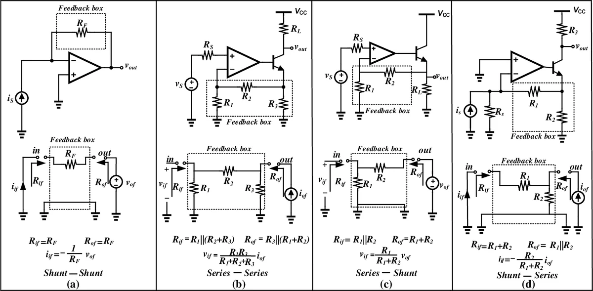
In Section II the authors introduce a systematic four‑step procedure: (1) identify the feedback topology by matching the circuit to one of four canonical configurations (series‑series, series‑shunt, shunt‑series, shunt‑shunt) using the visual taxonomy shown in Figures 1 and 2; (2) isolate the feedback network and represent it as a voltage or current source as appropriate; (3) determine loading effects by simple open‑circuit/short‑circuit inspection rather than memorizing Y, Z, h, g parameters; and (4) compute input and output impedances. This visual‑inspection method replaces the need to recall specific two‑port parameters, thereby reducing cognitive load. An illustrative example of shunt‑series feedback (Fig. 3) demonstrates how the input resistance (R_{if}=R_1+R_2) and output resistance (R_{of}=R_1\parallel R_2) follow directly from the open/short conditions indicated in the diagram.

Section III tackles the core technical contribution: a rigorous derivation of the output impedance for two variants of output‑series feedback. The authors first replace the preceding stages of the amplifier with a Thevenin equivalent ((v_{th}=K,v_{in}), (r_{th}=r_{out})). They then define the “output branch” comprising the series resistance (R_1) (or (R_2) in the second variant), the intrinsic output resistance (r_{out}), and the transistor small‑signal resistance (r_\pi\beta). Adding the feedback network multiplies this branch resistance by the factor ((1+af)), where (a) is the open‑loop gain and (f) the feedback factor.

For the first configuration (collector output, emitter‑sensing feedback) the authors obtain: \