Robust Tensor Recovery with Fiber Outliers for Traffic Events

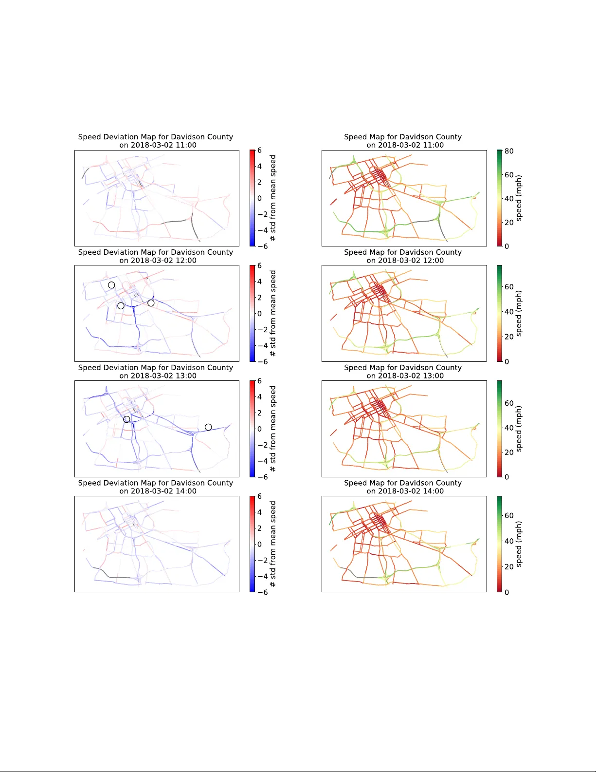
R O B U S T T E N S O R R E C O V E RY W I T H F I B E R O U T L I E R S F O R T R A FFI C E V E N T S A P R E P R I N T Y ue Hu V anderbilt Uni versity Nashville, TN37212 yue.hu@vanderbilt.edu Daniel W ork V anderbilt Uni versity Nashville, TN37212 dan.work@vanderbilt.edu August 28, 2019 A B S T R AC T Event detection is gaining increasing attention in smart cities research. Large-scale mobility data serves as an important tool to uncov er the dynamics of urban transportation systems, and more often than not the dataset is incomplete. In this article, we de velop a method to detect e xtreme e vents in large traffic datasets, and to impute missing data during regular conditions. Specifically , we propose a robust tensor recov ery problem to recover low rank tensors under fiber -sparse corruptions with par- tial observ ations, and use it to identify ev ents, and impute missing data under typical conditions. Our approach is scalable to large urban areas, taking full advantage of the spatio-temporal correlations in traffic patterns. W e dev elop an ef ficient algorithm to solve the tensor recov ery problem based on the alternating dir ection method of multipliers (ADMM) framew ork. Compared with existing l 1 norm regularized tensor decomposition methods, our algorithm can exactly recov er the v alues of uncor- rupted fibers of a lo w rank tensor and find the positions of corrupted fibers under mild conditions. Numerical experiments illustrate that our algorithm can exactly detect outliers e ven with missing data rates as high as 40%, conditioned on the outlier corruption rate and the Tuck er rank of the low rank tensor . Finally , we apply our method on a real traffic dataset corresponding to downto wn Nashville, TN, USA and successfully detect the events like sev ere car crashes, construction lane closures, and other large e vents that cause significant traf fic disruptions. K eywords rob ust tensor recov ery , tensor factorization, multilinear analysis, outlier detection, traf fic e vents, urban computing 1 Introduction 1.1 Motivation Event detection is an increasing interest in urban studies [1, 2]. Efficiently analyzing the impact of lar ge ev ents can help us assess the performance of urban infrastructure and aid urban management. Now adays, with the dev elopment of intelligent transportation systems, large scale traf fic data is accumulating via loop detectors, GPS, high-resolution cameras, etc. The lar ge amount of data provides us insight into the dynamics of urban environment in face of lar ge scale events. The main objectiv e of this article is to dev elop a method to detect extreme ev ents in traffic datasets describing large urban areas, and to impute missing data during re gular conditions. There are two major challenges in ev ent detecting outliers in traf fic datasets. Firstly , most large traf fic datasets are incomplete [3, 4, 5], meaning there are a large number of entries for which the current traffic condition is not kno wn. The missing data can be caused by the lack of measurements (e.g., no instrumented vehicles recently drove over the road segment), or due to senor failure (e.g., a traffic sensor which loses communication, power , is physically damaged). Missing data can hea vily influence the performance of traf fic estimation [4, 5, 6, 7], especially as the missing data rate increases. Naiv e imputation of the missing entries to create a complete dataset is problematic, because without a clear A P R E P R I N T - A U G U S T 2 8 , 2 0 1 9 hour of wee k ( h) 1 2 3 … 167 168 segment 1 segment 2 segment 3 road segment # week # week 2 week 3 … week N … segment !𝐼 # week 1 Figure 1: T raffic data is arranged in three-way tensor , with the dimensions corresponding to i ) the hour of the week, ii ) the road segment number , and iii ) the week number . understanding of the overall pattern, an incorrect v alue can be imputed that will later de grade the performance of an outlier detection algorithm. Consequently , missing data should be carefully handled. The second challenge is to fully capture and utilize the pattern of regular traffic, in order to correctly impute missing data and separate the outliers out from regular traffic. Studies hav e suggested that for regular traf fic patterns, there exist systematic correlations in time and space [8, 9, 10, 11]. For example, due to daily commute patterns, traffic conditions during Monday morning rush hour are generally repeated b ut with small variation from one week to the next (e.g., the rush hour might start a little earlier or last a little longer). Also, traffic conditions are spatially structured due to the network connectivity , ending up in global patterns. For example, the traf fic volume on one road segment should influence and be influenced by its down stream and upper stream traf fic v olume. Most existing researches have not fully addressed these two challenges. On the one hand, missing data and outlier detection tend to be dealt with separately . Either it is assumed that the dataset is complete, for the purpose of outlier detection [12, 13], or it is assumed that the dataset is clean, for the purpose of missing data imputation [14, 15]. Y et in reality missing data and outliers often exist at the same time. On the other hand, currently most studies on traffic outliers consider only a single monitor spot or a small region [16, 17, 18, 19], not fully exploiting the spatio- temporal correlations. Only a few studies scale up to large regions to capture the urban-wise correlation, including the work of Y ang et al. [8] proposing a coupled Bayesian r ob ust principal component analysis (robust PCA or RPCA) approach to detect road traf fic ev ents, and Liu et al. [20] constructing a spatio-temporal outlier tree to discov er the causal interactions among outliers. In this article, we tackle the traffic outlier ev ent detection problem from a different perspecti ve, taking into account missing data and spatio-temporal correlation. Specifically , we model a robust tensor decomposition problem, as illus- trated in subsection 1.2. Furthermore, we dev elop an ef ficient algorithm to solve it. W e note that the application of our method is not limited to traf fic e vent detection, b ut can also be applied to general pattern recognition and anomaly detection, where there exist multi-way correlations in the dataset, and in either full or partial observ ations. 1.2 Solution approach In this subsection, we dev elop the rob ust tensor decomposition model for traf fic extreme e vent detection problem, and dev elop a robust tensor completion problem to tak e partial observation into account. T o exploit these temporal and spatial structures, a tensor [21, 22] is introduced to represent the traffic data ov er time and space. W e form a three-way tensor, as shown in Figure 1. The first dimension is the road segment, the second dimension is the time of the week, (Monday Midnight-1am all the way to Sunday 11pm-midnight, 24 × 7 = 168 entries in total), and the third dimension is the week in the dataset. In this way , the temporal and spacial patterns along different dimensions are naturally encoded. One ef fective way to quantify this multi-dimensional correlation is the T ucker rank of the tensor [21, 22, 23], which is the generalization of matrix rank to higher dimensions. 2 A P R E P R I N T - A U G U S T 2 8 , 2 0 1 9 hour of w e e k ( h) segment 1 segment 2 segment 3 road segment # week # week 2 week 3 … week N … segment !𝐼 # week 1 hour of week (h) 1 2 3 … 167 168 segment 1 segment 2 segment 3 road segment # week # week 2 week 3 … week N … segment !𝐼 # week 1 1 2 3 … 167 168 hour of w e e k ( h) segment 1 segment 2 segment 3 road segment # week # week 2 week 3 … week N … segment !𝐼 # week 1 1 2 3 … 167 168 Figure 2: Observation data decomposed into low rank tensor for regular traffic and fiber-sparse tensor for outlier ev ents. As for the extreme ev ents, we expect them to occur relativ ely infrequently . W e encode the outliers in a sparse tensor , which is org anized in the same way as the traf fic data tensor . Furthermore, extreme ev ents tend to affect the overall traffic of an urban area. That is, we assume that at the time when extreme ev ent occurs, the traf fic data of all road se g- ments deviates from the normal pattern. Thus, the outliers occur sparsely as fibers along the road segment dimension with hour of week fixed. This sets it apart from random noises, which appear scattered ov er the whole tensor entries and unstructured. This fiber-wise sparsity problem is studied in 2D matrix cases [24], where the l 2 , 1 norm is used to control the column sparsity , and we adapt it for higher dimensions. Putting these together , we organize the traf fic data into a tensor B , then decompose it into two parts, B = X + E , where tensor X contains the data describing the regular traffic patterns, and tensor E denotes the outliers, as illustrated in Figure 2. Because the normal traf fic patterns is assumed to have strong correlation in time and space, it is approxi- mated by a low rank tensor X , Similarly , because outliers are infrequent, we e xpect the tensor containing outliers, E , to be sparse. W ith these ideas in mind, it is possible formulate the following optimization problem: min X , E rank ( X ) + λ sparsity ( E ) s.t. B = X + E . (1) The objectiv e function in problem (1) is the weighted cost of tensor rank of X denoted as rank( X ), the fiber-wise sparsity of E is denoted as sparsity( E ), and λ is a weighting parameter balancing the two costs. A more precise formulation of the problem is provided in Section 4. In the presence of missing data, we require the decomposition to match the observation data only at the av ailable entries, and come to the optimization problem: min X , E rank ( X ) + λ sparsity ( E ) s.t. B i 1 i 2 ...i N = ( X + E ) i 1 i 2 ...i N , where ( i 1 , i 2 , . . . , i N ) is an observed entry . (2) In this paper , we turn problem (1) and (2) into con vex programming problems, and solve them by extending from matrix case to tensor case a singular v alue thresholding algorithm [25, 26] based on alternating dir ection method of multipliers (ADMM) frame work. Our algorithm can e xactly reco ver the values of uncorrupted fibers of the lo w rank tensor , and find the positions of corrupted fibers, based on relatively mild condition of observation and corruption ratio. 1 1.3 Contributions and outline T o summarize, this work has three main contributions: 1 The resulting source code is av ailable at https://github.com/Lab- Work/Robust_tensor_recovery_for_traffic_ events . 3 A P R E P R I N T - A U G U S T 2 8 , 2 0 1 9 1. W e propose a new robust tensor recov ery with fiber outliers model for traffic extreme e vent detection under full or partial observations, to tak e full advantage of spatial-temporal correlations in traf fic pattern. 2. W e propose ADMM based algorithms to solve the rob ust tensor reco very under fiber-sparse corruption. Our algorithm can exactly reco ver the values of uncorrupted fibers of the lo w rank tensor, and find the positions of corrupted fibers under mild conditions. 3. W e apply our method on a large traf fic dataset in downto wn Nashville and successfully detect large e vents. The rest of the paper is organized as follows. In Section 3, we provide a revie w of tensor basics and related robust PCA methods. In Section 4, we formulate the tensor outlier detection problem, and propose efficient algorithms to solve it. In Section 5, we demonstrate the effecti veness of our method by numerical experiments. In Section 6, we apply our method on real world data set and sho w its ability to find large scale e vents. 2 Related work In this section, we describe literature on outlier detection. W e also compare our methodology with other relev ant works. 2.1 outlier detection The outliers we are interested in this work are due to outliers caused by extreme ev ents. Another related problem considers methods to detect outliers caused by data measurement errors, such as sensor malfunction, malicious tam- pering, or measurement error [17, 18, 27]. The latter methods can be seen as a part of a standard data cleaning or data pre-processing step. On the other hand, outliers caused by extreme traffic ha ve valuable information for congestion management, and can pro vide agencies with insights into the performance of urban network. The w orks [20, 28, 29] explore the problem of outlier detection caused by e vents, while the works [1, 30, 31, 32] focus on determining the root causes of the outlier . 2.2 Low rank matrix and tensor learning Low rank matrix and tensor learning has been widely used to utilize the inner structure of the data. V arious application hav e benefited from matrix and tensor based methods, including data completion [9, 33], link prediction [34], network structure clustering [35], etc. The most relev ant works with ours are rob ust matrix and tensor PCA for outlier detection. l 1 norm regularized robust tensor recovery , as proposed by Goldfarb and Qin [22], is useful when data is polluted with unstructured random noises. T an et al. [36] also used l 1 norm regularized tensor decomposition for traffic data recovery , in face of random noise corruption. But if outliers are structured, for example grouped in columns, l 1 norm regularization does not yield good results. In addition, although traffic is also modeled in tensor format in [36], only a single road segment is considered, not taking into account network spacial structures. In face of large e vents, outliers tend to group in columns or fibers in the dataset, as illustrated in section 1.2. l 2 , 1 norm regularized decomposition is suitable for group outlier detection, as shown in [24, 37] for matrices, and [38, 39] for tensors. In addition, Li et al. [40] introduced a multi-vie w lo w-rank analysis frame work for outlier detection, and W en et al. [2] used discriminant tensor factorization for event analytics. Our methods differ from the existing tensor outliers pursuit [38, 39] in that they are dealing with slab outliers, i.e., outliers form an entire slice instead of fibers of the tensor . Moreover , compared with existing works, we take one step further and deal with partial observ ations. As stated in Section 1.1, without an overall understanding of the underlying pattern, we can easily impute the missing entries incorrectly and influence our decision about outliers. W e will show in Section 5.3 simulation that our new algorithm can exactly detect the outliers e ven with 40% missing rate, conditioned on the outlier corruption rate and the rank of the low rank tensor . 3 Preliminaries In this section, we briefly revie w the mathematical preliminaries for tensor factorization, adopting the notation of K olda and Bader [21], and Goldfarb and Qin [22]. W e also summarize rob ust PCA [26], since it serves as a foundation for our extension to higher -order tensor decomposition. 4 A P R E P R I N T - A U G U S T 2 8 , 2 0 1 9 3.1 T ensor basics In this article, a tensor is denoted by an Euler script letter (e.g., X ); a matrix by a boldface capital letter (e.g., X ); a vector by a boldface lowercase letter (e.g., x ); and a scalar by a lowercase letter (e.g., x ). A tensor of order N has N dimensions, and can be equi valently described as an N -way tensor or an N -mode tensor . Thus, matrix is a second order tensor , and vector is a first order tensor . A fiber is a column vector formed by fixing all indices of a tensor but one. In a matrix for e xample, each column can be viewed as a mode-one fiber , and each ro w a mode-two fiber . The unfolding of a tensor X in the n th mode results in a matrix X ( n ) , which is formed by rearranging the mode- n fibers as its columns. This process is also called flattening or matricization. The in verse function of unfolding is denoted as fold n ( · ) , i.e., fold n ( X ( n ) ) = X . The inner pr oduct of two tensors X , Y ∈ R I 1 × I 2 ×···× I N is the sum of their element-wise product, similar to vector inner products. Let x i 1 i 2 ...i N and y i 1 i 2 ...i N denote the ( i 1 , i 2 , · · · , i N ) element of X and Y respectively . Then tensor inner product can be expressed as hX , Y i = I 1 X i 1 =1 I 2 X i 2 =1 · · · I N X i N =1 x i 1 i 2 ...i N y i 1 i 2 ...i N . The tensor F r obenius norm is denoted by k · k F , and computed as kX k F = p hX , X i . Multiplication of a tensor by a matrix in mode n is performed by multiplying ev ery mode- n fiber of the tensor by the matrix. The mode- n product of a tensor X ∈ R I 1 × I 2 ×···× I N and a matrix A ∈ R J × I n is denoted by X × n A = Y , where Y ∈ R I 1 × I 2 ×···× I n − 1 × J × I n +1 ×···× I N . It is also equiv alently written via its mode- n unfolding as Y ( n ) := AX ( n ) . The T ucker decomposition [21, 22] is the generalization of matrix PCA in higher dimensions. It approximates a tensor X ∈ R I 1 × I 2 ×···× I N as a core tensor multiplied in each mode n by an appropriately sized matrix U ( n ) : X ≈ G × 1 U (1) × 2 U (2) × · · · × N U ( N ) . (3) G ∈ R c 1 × c 2 ×···× c N in (3) is called the core tensor , where c 1 through c N are given integers. If c n < I n for some n in (1 , 2 , . . . , N ) , the core tensor G can be vie wed as a compressed version of X . The matrices U ( n ) ∈ R I n × c n are factor matrices, which are usually assumed to be orthogonal. The n-rank of X , denoted by rank n ( X ) , is the column rank of X ( n ) . In other words, it is the dimension of the vector space spanned by the mode- n fibers. If we denote the n -rank of the tensor X as R n for n = 1 , 2 , . . . , N , i.e., R n = rank n ( X ) , then the set of the N n -ranks of X , ( R 1 , R 2 , . . . , R N ) , is called the T ucker Rank [21]. In T ucker decomposition (3), if c n = rank n ( X ) for all n in (1 , 2 , . . . , N ) , then the T ucker decomposition is exact. In this case, we can easily conduct the decomposition by setting U ( n ) as the left singular matrix of X ( n ) . Otherwise, if c n < rank n ( X ) , the decomposition holds only as an approximation, and will be harder to be solved. 3.2 Robust PCA W e briefly summarize robust v ariants of PCA in the matrix setting, which are extended to higher -order tensor settings in Section 4. Robust PCA belongs to the family of dimension-reduction methods aiming at combating the so-called curse of dimensionality that often appears when dealing with large, high dimensional datasets, by finding the best representing low-dimensional subspace. PCA is a widely used technique in this family , yet it is sensitiv e to corrup- tions [26]. For example, if we hav e a large data matrix that comes from a lo w rank matrix randomly corrupted by large noises, i.e., B = X + E , where B ∈ R I 1 × I 2 is the data matrix, X ∈ R I 1 × I 2 is a lo w rank matrix, and E ∈ R I 1 × I 2 is a sparse corruption matrix of arbitrary magnitude. In this setting traditional PCA fails at finding the subspace for X giv en only B . T o address the problem of gross corruption, Cand ` es et al. [26] proposed a RPCA method known as Principle Compo- nent Pursuit (PCP): 5 A P R E P R I N T - A U G U S T 2 8 , 2 0 1 9 min X , E k X k ∗ + λ k E k 1 s.t. B = X + E , (4) with the l 1 matrix norm k · k 1 of E giv en by: k E k 1 := I 1 X i =1 I 2 X j =1 | e ij | , and where e i,j denotes the ( i, j ) th element of E . The nuclear norm of a matrix X is denoted as k · k ∗ and is computed as the sum of the singular values of X : k X k ∗ := X i σ i . where the SVD of X is X = P i σ i u i v T i . The nuclear norm in (4) is proposed as the tightest con vex relaxation of matrix rank [25]; and the l 1 norm is the con ve x approximation for element-wise matrix sparsity . Cand ` es et al. [26] showed that PCP can e xactly recov er a lo w rank matrix when it is grossly corrupted at sparse entries. Moreover , by adopting ADMM algorithm, it is possible to solve (4) in polynomial time. The PCP formulation (4) requires incoherence of the column space of the sparse matrix E [24, 26], and does not address the setting where entire columns are corrupted. An alternati ve problem formulation using an l 2 , 1 norm on E in (4) is introduced for matrix recov ery with column-wise corruption [24, 37]. The l 2 , 1 norm of a matrix E ∈ R I 1 × I 2 is defined as k E k 2 , 1 = I 2 X j =1 v u u t I 1 X i =1 ( e ij ) 2 . It is essentially a form of group lasso [41], where each column is treated as a group. Minimizing k E k 2 , 1 encourages the entire columns of E to be zero or non-zero, and leads to fewer non-zero columns. Note that it is hard to reco ver an uncorrupted column from a completely corrupted one. Therefore, instead of trying to recov er the complete low rank matrix, Xu et al. [24] seeks instead to recover the exact low-dimensional subspace while identifying the location of the corrupted columns. T ang et al. [37] makes an assumption that if a column is corrupted (i.e., E has nonzero entries in this column), then the entries of the corresponding column in the lo w-rank matrix X are zero. This choice allows e xact recovery of the lo w rank matrix in the non-corrupted columns. Like PCA for a matrix, we note that the T ucker decomposition of a tensor is also sensiti ve to gross corruption [22]. Motiv ated by the ideas of Cand ` es et al. [26] and T ang [37] for robust matrix PCA, in the next section we address the problem of robust decomposition of tensors with gross fiber -wise corruption. 4 Methods In this section, we define and pose the higher-order tensor decomposition problem in the presence of fiber outliers and its partial-observation v ariant as con ve x programs, and provide ef ficient algorithms to solve them. 4.1 Problem f ormulation The precise setup of the problem is as follows. W e are given a high dimensional data tensor B ∈ R I 1 × I 2 ×···× I N which is composed of a low-rank tensor X ∈ R I 1 × I 2 ×···× I N that is corrupted in a few fibers. In other words, we hav e B = X + E , where E ∈ R I 1 × I 2 ×···× I N is the sparse fiber outlier tensor . W e know neither the rank of X , nor the number and position of non-zero entries of E . Giv en only B , our goal is to reconstruct X on the non-corrupted fibers, as well as identify the outlier location. Moreov er , we might hav e only partial observ ations of B , and we seek to complete the decomposition nev ertheless. W e do assume knowledge of the mode along which the fiber outliers are distributed; without loss of generality let it be the first dimension. Then it is equiv alent to say the mode-1 unfolding of the outlier tensor is column-wise sparse. Thus, we can formulate the problem as: min X , E rank ( X ) + λ k E (1) k 2 , 1 s.t. B = X + E . (5) 6 A P R E P R I N T - A U G U S T 2 8 , 2 0 1 9 Computing the rank of a tensor X , denoted by rank( X ) is generally an NP-hard problem [22, 42]. One commonly used con vex relaxation of the tensor rank is P i k X ( i ) k ∗ , which sums the nuclear norm of the tensor unfoldings in all modes [22]. In this way , we generalize the matrix nuclear norm to the higher -order case, and e xplore the potential low rank structure in all dimensions. Problem (5) thus becomes min X , E N X i =1 k X ( i ) k ∗ + λ k E (1) k 2 , 1 s.t. B = X + E . (6) Next, we deal with the case when the data is only partially av ailable, in addition to observ ation data being grossly corrupted. W e only know the entries ( i 1 , i 2 , . . . , i N ) ∈ Ω , where Ω ⊂ [ I 1 ] × [ I 2 ] × · · · × [ I N ] is an observ ation index set. Let X Ω denote the projection of X onto the tensor subspace supported on Ω . Then X Ω can be defined as X Ω =  X i 1 i 2 ...i N , ( i 1 , i 2 , . . . , i N ) ∈ Ω 0 , otherwise. Then we can force the decomposition to match the observation data only at the available entries, and find the decom- position that minimizes the weighted cost of tensor rank and sparsity , leading to the follo wing model: min X , E N X i =1 k X ( i ) k ∗ + λ k E (1) k 2 , 1 s.t. B Ω = ( X + E ) Ω . (7) Note that related problems to (7) for the matrix setting are addressed in [26, 43]). 4.2 Algorithm In this section, we de velop algorithm for tensor decomposition with fiber-wise corruption model formulated in Sec- tion 4.1. W e first solve (6) for the full-observ ation setting, then for the partial-observ ation setting (7), adopting an ADMM method [22] for each. 4.2.1 Higher -order RPCA Problem (6) is difficult to solve because the terms k X ( i ) k ∗ in the objective function are interdependent, since each X ( i ) is unfolded from the same tensor X . Alternativ ely , we split X into N auxiliary variables, X 1 , X 2 , . . . , X N ∈ R I 1 × I 2 ×···× I N , and rewrite (6) as: min X i , E N X i =1 k X i ( i ) k ∗ + λ k E (1) k 2 , 1 s.t. B = X i + E , i = 1 , 2 , . . . , N , (8) where X i ( i ) are the unfoldings of X i in the i th mode. The N constraints B = X i + E ensure that X 1 , X 2 , . . . , X N are all equal to the original X in problem (6). Next, we proceed to solv e problem (8) via an ADMM algorithm. A full explanation of the general ADMM framew ork can be found in [44]. The corresponding augmented Lagrangian function for problem (8) is L ( X 1 , X 2 , . . . , X N , E , Y 1 , Y 2 , . . . , Y N ; µ ) = N X i =1 k X i ( i ) k ∗ + λ k E (1) k 2 , 1 + N X i =1  µ 2 kX i + E − B ) k 2 F − hY i , X i + E − B i  . Here Y i are the Lagrange multipliers, and µ is a positiv e scalar . Under the ADMM framew ork, the approach is to iterativ ely update the three sets of variables ( X 1 , X 2 , . . . , X N ) , E , ( Y 1 , Y 2 , . . . , Y N ) . T o be specific, at the start of the k + 1 th iteration, we fix E = E k and Y i = Y k i , then for each i solve: X k +1 i = argmin X i L ( X i , E k , Y k i ; µ ) . (9) 7 A P R E P R I N T - A U G U S T 2 8 , 2 0 1 9 Then, we fix X i = X k +1 i and Y i = Y k i to solve: E k +1 = argmin E L ( X k +1 i , E , Y k i ; µ ) . (10) Finally we fix X i = X k +1 i and E = E k +1 , and update Y k i : Y k +1 i = Y k i + µ ( B − X k +1 i − E k +1 ) . (11) Next we deri ve closed form solutions for problem (9) and for problem (10). Problem (9), written out, reads: X k +1 i = argmin X i k X i ( i ) k ∗ + µ 2 kX i + E k − B ) k 2 F − hY k i , X i + E k − B i . (12) Using the property of the Frobenius norm, kA 1 + A 2 k 2 F = kA 1 k 2 F + kA 2 k 2 F + 2 hA 1 , A 2 i , problem (12) can be written as: X k +1 i = argmin X i k X i ( i ) k ∗ + µ 2     1 µ Y k i + B − E k − X i     2 F = argmin X i k X i ( i ) k ∗ + µ 2     1 µ Y k i ( i ) + B ( i ) − E k ( i ) − X i ( i )     2 F . (13) In the second line of (13), we change the Frobenius norm of a tensor into the Frobenius norm of its i -th unfolding, which does not change the actual value of the norm. As a result, the objective function of problem (13) only inv olves matrices, so we can solve for X i ( i ) using the well-established closed form solution (e.g., see proof in Cai et. al [25]): X k +1 i ( i ) = T 1 µ ( 1 µ Y k i ( i ) + B ( i ) − E k ( i ) ) . Then we fold the matrix X k +1 i ( i ) back into a tensor , i.e., X k +1 i = fold i ( X k +1 i ( i ) ) . The truncation operator T τ ( X ) in for a matrix X = U Σ V T is T τ ( X ) = U Σ ¯ τ V T , where Σ = diag ( σ i ) is the eigen value diagonal matrix for X . The operation Σ ¯ τ = diag(max ( σ i − τ , 0)) discards the eigen v alues less than τ , and shrinks the remaining eigen values by τ . W e now proceed to deri ve a closed form solution to update E in problem (10). Problem (10) is equiv alent to solving: E k +1 = argmin E λ k E (1) k 2 , 1 + N X i =1 ( µ kX k +1 i + E − B ) k 2 F − hY k i , X k +1 i + E − B i ) . (14) Follo wing the same technique as earlier , (14) is equiv alent to: E k +1 = argmin E λ k E (1) k 2 , 1 + N X i =1 µ 2     1 µ Y k i + B − X k +1 i − E     2 F ! . (15) By the proof of Goldfarb and Qin [22], problem (15) shares the same solution with: E k +1 = argmin E λ   E (1)   2 , 1 + µN 2      E − 1 N N X i =1  1 µ Y k i + B − X k +1 i       2 F , (16) since they have the same first-order conditions. In order to simplify expression (16), we denote the term 1 N P N i =1  1 µ Y k i + B − X k +1 i  by a single variable C ∈ R I 1 × I 2 ×···× I N . Thus, E k +1 = argmin E λ k E (1) k 2 , 1 + µN 2 kE − C k 2 F = argmin E λ k E (1) k 2 , 1 + µN 2 k E (1) − C (1) k 2 F , (17) where in the second line we use the same approach as in (13) in which we replace the tensor Frobenius norm by the equiv alent Frobenius norm of the mode one unfolding. The objecti ve function of problem (17) only in volv es matrices, and the closed form solution is [37]: E k +1 (1) j = C (1) j max  0 , 1 − λ µN k C (1) j k 2  , for j = 1 , 2 , . . . , p, (18) where E (1) j is the j th column of E (1) , C (1) j is the j th column of C (1) , and the inte ger p = I 2 × I 3 × · · · × I N is the total number of columns in C (1) . This operation effecti vely sets a column of C (1) to zero if its l 2 norm is less than λ µN , and scales the elements down by a f actor 1 − λ µN k C (1) j k 2 otherwise [37]. 8 A P R E P R I N T - A U G U S T 2 8 , 2 0 1 9 Algorithm 1 T ensor robust PCA for fiber-wise corruptions 1: Gi ven B , λ, µ . Initialize X i = E = Y i = 0 . 2: f or k = 0 , 1 , . . . do 3: for i = 1 : N do  Update X 4: X k +1 i ( i ) = T 1 µ  1 µ Y k i ( i ) + B ( i ) − E k ( i )  . 5: X k +1 i = fold i  X k +1 i ( i )  6: end for 7: C = 1 N P N i =1  1 µ Y k +1 i + B − X k +1 i   Update E . 8: for j = 1 , 2 , . . . , p do 9: E k +1 (1) j = C (1) j max n 0 , 1 − λ µN k C (1) j k 2 o 10: end for 11: E k +1 = fold 1 ( E k +1 (1) ) 12: for i = 1 : N do  Update Y . 13: Y k +1 i = Y k i + µ ( B − X k +1 i − E k +1 ) . 14: end for 15: end f or 16: r eturn X k = 1 N P N i =1 X k i , E k Note that compared with the ADMM method where we just update X i and E once, the augmented Lagrangian multi- pliers (ALM) method [45] seeks to find the exact solutions for primal variables X i and E before updating Lagrangian multipliers Y i = Y k i , yielding the framew ork as ( X k +1 i , E k +1 ) = argmin X i , E L ( X i , E , Y k i ; µ ) Y k +1 i = Y k i + µ ( B − X k +1 i − E k +1 ) . As pointed out by Lin et al. [45], compared with ALM, not only is ADMM still able to con v erge to the optimal solution for X i and E , but also the speed performance is better . It is also noted that while in ALM, the X and E are optimized jointly , in the ADMM implementation, they are in fact updated sequentially [44]. It is often observed in the matrix settings (see e.g., Lin et al. [45]) that updating the term containing outliers before the low rank term (i.e., E before X in the tensor setting) the low rank term results in faster conv ergence. As a consequence this is the approach followed in the numerical implementation of Algorithm 1 used later in this work. In the implementation of Algorithm 1, we set the con ver gence criterion as kB − E − X k F kB k F ≤ , (19) Where  is the tolerance. 4.2.2 Partial Observ ation Now we provide an algorithm to solve problem (7). Similar to the matrix setting in T ang et al. [37], we set the fibers of the low rank tensor to be zero in the locations corresponding to outliers. W e introduce a compensation tensor O ∈ R I 1 × I 2 ×···× I N , which is zero for entries in the observation set Ω , and can take any value outside Ω . Thus using the same auxiliary variables technique as in (8), we can reformulate problem (7) as: min X i , E N X i =1 k X i ( i ) k ∗ + λ k E (1) k 2 , 1 s.t. B = X i + E + O , i = 1 , 2 , . . . , N , O Ω = 0 . (20) Since O compensates for whatev er the value is in the unobserved entries of B , we only need to keep track of the indices of the unobserved entries, and can simply set the unobserved entries of B to zero. The augmented Lagrangian 9 A P R E P R I N T - A U G U S T 2 8 , 2 0 1 9 Algorithm 2 ADMM for robust tensor completion 1: Gi ven B , λ, µ . Initialize X i = E = Y i = O = 0 . 2: f or k = 0,1, · · · do 3: for i = 1:N do  Update X 4: X k +1 i ( i ) = T 1 µ ( B ( i ) + 1 µ Y k i ( i ) − E k ( i ) − O k ( i ) ) , 5: X k +1 i = fold i ( X k +1 i ( i ) ) 6: end for 7: C = 1 N P N i =1  1 µ Y k +1 i + B − X k +1 i − O k +1   Update E . 8: for j = 1 , 2 , . . . , p do 9: E k +1 (1) j = C (1) j max n 0 , 1 − λ µN k C (1) j k 2 o 10: end for 11: E k +1 = fold 1 ( E k +1 (1) ) 12: O k +1 =  P N i = i  1 µ Y k i + B − X k +1 i − E k +1  Ω C .  Update O . 13: for i = 1 : N do  Update Y . 14: Y k +1 i = Y k i + µ ( B − X k +1 i − E k +1 − O k +1 ) 15: end for 16: end f or 17: r eturn X k = 1 N P N i =1 X k i , E k function for problem (20) is L ( X 1 , X 2 , . . . , X N , E , O , Y 1 , Y 2 , . . . , Y N ; µ ) = N X i =1 k X i ( i ) k ∗ + λ k E (1) k 2 , 1 + N X i =1  µ 2 kX i + E + O − B ) k 2 F − hY i , X i + E + O − B i  . W e again use the ADMM frame work no w iterativ ely updating X i , E , O and Y i . The proof of the closed form solution for updating X i , E and Y i is similar to Algorithm 1. For O , we fix X i = X k +1 i , E = E k +1 and Y i = Y k i , to solve (21): O k +1 = argmin O L ( X k +1 i , E k +1 , O , Y k i ; µ ) s.t. O Ω = 0 . (21) Follo wing the same procedure as before (see (14), (15) and (16)), we hav e: O k +1 = argmin O N X i =1  µ 2   X k +1 i + E k +1 + O − B )   2 F − hY k i , X k +1 i + E k +1 + O − B i  = argmin O N X i =1 µ 2     1 µ Y k i + B − X k +1 i − E k +1 − O     2 F ! = argmin O µN 2      O − 1 N N X i =1  1 µ Y k i + B − X k +1 i − E k +1       2 F , s.t. O Ω = 0 . (22) For (22), we simply set O = 1 N P N i =1 ( 1 µ Y k i + B − X k +1 i − E k +1 ) for entries ( I 1 , I 2 , . . . , I N ) ∈ Ω C , and zero otherwise. The procedure is summarized in Algorithm 2. W e set the con vergence criterion of Algorithm 2 as kB − E − X − O k F kB k F ≤ , which is similar to (19) but accounts for the additional tensor O . 10 A P R E P R I N T - A U G U S T 2 8 , 2 0 1 9 5 Numerical experiments In this section, we apply Algorithms 1 and 2 dev eloped in Section 4.2 on a series of test problems using synthetically generated datasets. W e first conduct tensor decomposition on fiber-wise corrupted data, then we examine the case when the data is only partially observed and is also fiber -wise corrupted. For both cases, we compare the performance of our algorithms, which are l 2 , 1 norm constrained decomposition, with l 1 norm constrained decomposition [22, 36]. W e demonstrate via the numerical experiments that our algorithms are able to exactly recover the original low-rank tensor , and identify the position of corrupted fibers. In comparison, l 1 norm constrained algorithms performs poorly in the fiber-wise corrupted settings, unable to achie ve e xact recoveries. 5.1 Perf ormance measures and implementation For each of the numerical experiments, the performance of the algorithms are measured by the relativ e error of the low rank tensor , as well as the precision and recall of the outlier fibers. The r elative error (RE) of low rank tensor is calculated as: RE = kX 0 − ˆ X k F kX 0 k F , where X 0 is the true low rank tensor modified to take the value 0 in the entries corresponding to the corrupted fibers; ˆ X is the estimated low rank tensor resulting from application of Algorithm 1 or 2, which also has the value 0 in the fibers that are estimated to be corrupted. W e compute the pr ecision of the algorithm to assess the potential to correctly identify only the outlier fibers. It is computed as: precision = tp tp + fp , where the true positives (tp) corresponds the number of estimated outlier fibers which are true outliers, and the false positives (fp) corresponds to the number of estimated outlier fibers which are not true outliers. The r ecall , which measures the ability to find all outlier fibers, is defined as recall = tp tp + fn , where the false negatives (fn) correspond to the number of true outlier fibers that were not correctly identified by the estimator . For the conv ergence criterion we set  = 10 − 7 , and we use an empirical value λ = 1 0 . 03 I m , where I m = max ( I 1 , . . . , I N ) . The hyperparameter λ in l 1 norm constrained decomposition algorithm is also tuned for its best performance in our settings. All of the experiments are carried out on a Macbook Pro with quad-core 2.7GHz Intel i7 Processor and 16GB RAM, running Matlab R2018a. W e modify and extend the code of Lin et. al [45], using PR OP A CK toolbox to efficiently calculate the SVD. The code is modified to update variables in line with the distinct problem formulation using the l 2 , 1 norm and to scale to tensors rather than matrices. The T ensor T oolbox for Matlab [46] [47] is also used for tensor manipulations. The resulting source code is av ailable at https://github.com/Lab- Work/Robust_tensor_ recovery_for_traffic_events . 5.2 T ensor rob ust PCA In this subsection we apply higher-order RPCA to the problems where we have fully observed data with fiber-wise corrupted entries. 5.2.1 Simulation conditions W e synthetically generate the observation data as B = X 0 + E 0 ∈ R I 1 × I 2 × I 3 , where X 0 and E 0 are the true or “ground truth” lo w-rank tensor and fiber-sparse tensor , respectiv ely . W e generate X 0 ∈ R I 1 × I 2 × I 3 as a core tensor G ∈ R c 1 × c 2 × c 3 with size c 1 × c 2 × c 3 and tucker rank ( c 1 , c 2 , c 3 ) , multiplied in each mode by orthogonal matrices of corresponding dimensions, U ( i ) ∈ R I i × c i : X 0 = G × 1 U (1) × 2 U (2) × 3 U (3) . 11 A P R E P R I N T - A U G U S T 2 8 , 2 0 1 9 T able 1: Application of Algorithm 1 on fiber-wise corrupted tensors with full observation, and comparison with l 1 norm constrained decomposition. For different tensor sizes ( I 1 , I 2 , I 3 ) and T ucker ranks ( c 1 , c 2 , c 2 ) , where we set c = 0 . 1 I , we show the relati ve errors of lo w rank tensors (RE), the precision and recall of outlier fibers identification, as well as the number of iterations (iter) and total time for con ver gence. (a) Algorithm 1: l 2 , 1 norm constrained decomposition ( I 1 , I 2 , I 3 ) ( c 1 , c 2 , c 2 ) RE precision recall iter time(s) (70,70,70) (7,7,7) 1 . 23 × 10 − 7 1.0 1.0 29 9.9 (90,90,90) (9,9,9) 1 . 24 × 10 − 7 1.0 1.0 28 16.2 (150,150,150) (15,15,15) 6 . 68 × 10 − 8 1.0 1.0 28 50.5 (210,210,210) (21,21,21) 7 . 35 × 10 − 8 1.0 1.0 28 133.0 (b) Comparison: l 1 norm constrained decomposition ( I 1 , I 2 , I 3 ) ( c 1 , c 2 , c 2 ) RE precision recall iter time(s) (70,70,70) (7,7,7) 2 . 10 × 10 − 1 1.0 1.0 28 1.4 (90,90,90) (9,9,9) 2 . 28 × 10 − 1 1.0 1.0 29 2.6 (150,150,150) (15,15,15) 2 . 23 × 10 − 1 1.0 1.0 28 14.7 (210,210,210) (21,21,21) 2 . 27 × 10 − 1 0.99 1.0 35 101.0 The entries of G are independently sampled from standard Gaussian distribution. The orthogonal matrices U ( i ) are generated via a Gram-Schmidt orthogonalization on c i vectors of size R I i drawn from standard Gaussian distrib ution. The sparse tensor E 0 ∈ R I 1 × I 2 × I 3 is formed by first generating a tensor E 0 0 ∈ R I 1 × I 2 × I 3 , whose entries are i.i.d uni- form distribution U (0,1). Then we randomly k eep a fraction γ of the fibers of E 0 0 to form E 0 . Finally , the corresponding fibers of X 0 with respect to non-zero fibers in E 0 are set to zero. 5.2.2 Algorithm performance f or varying pr oblem sizes W e apply Algorithm 1 on B of varying tensor sizes ( I 1 , I 2 , I 3 ) and underlying tucker rank ( c 1 , c 2 , c 3 ) , and predict ˆ X and ˆ E using Algorithm 1. W e also apply l 1 norm constrained decomposition on the same settings. T able 1 compares the result. The corruption rate is set to 5% , i.e., γ = 0 . 05 . In all cases, for our algorithm the relativ e residual errors are less than 10 − 6 , which is the same precision that we set for con ver gence tolerance. That is to say , we can exactly recov er the low rank tensors in this setting. The precision and recall are both 1.0, indicating that the outlier detection is also e xact. Similar to the observ ation of Cand ` es’ et al. [26], the iteration numbers tend to be constant (between 28 and 29 in this case) regardless of tensor size. This indicates that the number of of SVD computations might be limited and insensitiv e to the size, which is important since SVD is the computational bottleneck of the algorithm. Furthermore, this property is important to allow the problem to solve quickly ev en on datasets of moderate sizes, as will be shown in a case study in Section 6. In comparison, although l 1 norm constrained decomposition can also detect outliers in high precision and recall, the relativ e residual errors are relativ ely , high, in the order of 10 − 1 . This indicates that l 1 norm constrained decomposition can do an adequate job when corruption ratio is low ( γ = 0 . 05 ), but cannot achie ve exact reco veries. 5.2.3 Influence of the corruption rate Next, we in vestigate the performance of Algorithm 1 as the corruption ratio changes, and compare the result with l 1 norm constrained decomposition. W e fix the low-rank tensor X 0 at size R 70 × 70 × 70 with a tucker rank of (5 , 5 , 5) , then vary the gross corruption ratio γ from 0% to 60%. The results are shown in Figure 3 as an av erage over 10 trials. In this setting we see that as long as the corruption ratio is belo w 0.47, Algorithm 1 can precisely recov er the lo w rank tensor , and correctly identify the outlier fibers. On the other hand, the relativ e error of l 1 norm constrained decomposition is constantly higher . After the corruption ratio exceeds 0.2, the estimation is no longer useful, with the relative error exceeding 100%. 12 A P R E P R I N T - A U G U S T 2 8 , 2 0 1 9 0 0.1 0.2 0.3 0.4 0.5 0.6 corruption ratio 0 5 10 15 20 25 30 35 RE RE v.s. corruption ratio for l 1 and l 2,1 norm regularizations l 1 norm l 2,1 norm regularization (a) 0 0.1 0.2 0.3 0.4 0.5 0.6 corruption ratio 0 10 20 30 40 # Iteration # Iteration v.s. corruption ratio for l 1 and l 2,1 norm regularizations l 1 norm l 2,1 norm regularization (b) 0 0.1 0.2 0.3 0.4 0.5 0.6 corruption ratio 0 0.2 0.4 0.6 0.8 1 Recall Recall v.s. corruption ratio for l 1 and l 2,1 norm regularizations l 1 norm l 2,1 norm regularization (c) 0 0.1 0.2 0.3 0.4 0.5 0.6 corruption ratio 0 0.2 0.4 0.6 0.8 1 Precision Precision v.s. corruption ratio for l 1 and l 2,1 norm regularizations l 1 norm l 2,1 norm regularization (d) Figure 3: Comparison of Algorithm 1 ( l 2 , 1 norm regularized tensor decomposition), with l 1 norm regularized tensor decomposition, as gross corruption rate changes. W e fix the tensor size at R 70 × 70 × 70 , and fix the tucker rank of low rank tensor X 0 at (5 , 5 , 5) , then vary the gross corruption ratio γ from 0% to 100%. The result is an av erage over 10 trials. 5.3 Robust tensor completion In this subsection we look at the performance of Algorithm 2, when the data is only partially observed, and compare it with l 1 norm constrained decomposition. 5.3.1 Simulation conditions W e first generate a full observation data B 0 = X 0 + E 0 ∈ R I 1 × I 2 × I 3 in the same way as Section 5.2. X 0 ∈ R I 1 × I 2 × I 3 is the low rank tensor, and E 0 ∈ R I 1 × I 2 × I 3 is the sparse tensor . Then, we form the partial observation data B ∈ R I 1 × I 2 × I 3 by randomly keeping a fraction ρ of the entries in B 0 . W e record the indices of the unobserved entries, and set their values in B as 0. 13 A P R E P R I N T - A U G U S T 2 8 , 2 0 1 9 0 0.2 0.4 0.6 0.8 1 observation ratio 0 0.2 0.4 0.6 0.8 1 RSE RSE v.s. observation ratio for different corruption ratios = 0.05 = 0.1 = 0.2 corruption ratio (a) 0 0.2 0.4 0.6 0.8 1 observation ratio 0 5 10 15 20 25 30 35 40 # Iteration # Iteration v.s. observation ratio for different corruption ratios = 0.05 = 0.1 = 0.2 corruption ratio (b) 0 0.2 0.4 0.6 0.8 1 observation ratio 0 0.2 0.4 0.6 0.8 1 Recall Recall v.s. observation ratio for different corruption ratios = 0.05 = 0.1 = 0.2 corruption ratio (c) 0 0.2 0.4 0.6 0.8 1 observation ratio 0 0.2 0.4 0.6 0.8 1 Precision Precision v.s. observation ratio for different corruption ratios = 0.05 = 0.1 = 0.2 corruption ratio (d) Figure 4: Results of Algorithm 1 as a function of observation ratio with dif ferent corruption rates. The lo w-rank tensor X 0 size is fixed at R 70 × 70 × 70 with a tucker rank of (5 , 5 , 5) , and the gross corruption ratio γ is set at 0.05, 0.1, or 0.2. The result is an av erage over 10 trials. 5.3.2 Influence of the corruption and observation ratios First, we apply Algorithm 2 on simulated data with a varying corruption ratio and observation ratio. W e fix the low- rank tensor X 0 at size R 70 × 70 × 70 with a tucker rank of (5 , 5 , 5) . For gross corruption ratio γ at 0.05, 0.1, 0.2, we v ary the observation ratio ρ from 0.1 to 1 and run Algorithm 2. W e run 10 times and av erage the results. Figure 4 shows that for the detection of corrupted fibers, the recall stays at 1. The precision stays at 1 when ρ is abov e 0.6 but drops dramatically for smaller ρ . The relative error of low rank tensor is zero when the observation ratio ρ > 0 . 6 with corruption ratio γ = 0 . 05 , and when the observ ation ratio ρ > 0 . 8 with γ = 0 . 1 . W e observe a phase-transition beha vior, in that the decomposition is e xact when the observ ation ratio ρ is abov e a critical threshold, but the performance drops dramatically below the threshold. This critical threshold on the observation ratio ρ v aries for each case, namely the algorithm can handle more missing entries as the number of outliers γ is reduced. But when the corruption ratio is too large, e xact recovery is not guaranteed. Overall, the performance is promising, since we can exactly identify the outlier positions and recov er the low rank tensor at non-corrupted entries, e ven with relati vely a large missing ratio, for example when 5% of the fibers are corrupted and 40% of the data is missing. 14 A P R E P R I N T - A U G U S T 2 8 , 2 0 1 9 0 0.2 0.4 0.6 0.8 1 observation ratio 0 0.2 0.4 0.6 0.8 1 RES RES v.s. observation ratio for different tucker ranks (8,8,8) (5,5,5) (2,2,2) tucker rank (a) 0 0.2 0.4 0.6 0.8 1 observation ratio 5 10 15 20 25 30 35 40 45 # Iteration # Iteration v.s. observation ratio for different tucker ranks (8,8,8) (5,5,5) (2,2,2) tucker rank (b) 0 0.2 0.4 0.6 0.8 1 observation ratio 0 0.2 0.4 0.6 0.8 1 Recall rate Recall v.s. observation ratio for different tucker ranks (8,8,8) (5,5,5) (2,2,2) tucker rank (c) 0 0.2 0.4 0.6 0.8 1 observation ratio 0 0.2 0.4 0.6 0.8 1 Precision Precision v.s. observation ratio for different tucker ranks (8,8,8) (5,5,5) (2,2,2) tucker rank (d) Figure 5: Results of Algorithm 2 as a function of the observation ratio considering X 0 with varying tucker rank. The low-rank tensor X 0 is generated with a tucker rank of (2,2,2), (5,5,5), and (8,8,8) respectiv ely , with a fixed size of R 70 × 70 × 70 , and a gross corruption ratio γ = 0 . 1 . The plotted result is an av erage over 10 trials. 5.3.3 Influence of the observation ratio and the tensor rank Next we fix the low-rank tensor X 0 at size R 70 × 70 × 70 and gross corruption ratio γ = 0 . 1 . For X 0 of different tucker ranks (2,2,2),(5,5,5), and (8,8,8), we vary the observation ratio from 0.1 to 1 and run Algorithm 2. The result is shown in Figure 5, which is an average across 10 trials. Ag ain, we observe a phase-transaction behavior , that when observation ratio is above a critical threshold, the decomposition is e xact, with precision and recall at one, and relativ e error at zero. For tensor ranks (5,5,5) and (8,8,8), this threshold is about 0.8. For tensor rank (2,2,2), it is lo wer , about 0.5. This indicates that when the underlying tensor rank is lo wer , we can exactly conduct the decomposition with ev en with a lower observ ation ratio. 5.3.4 Comparison with l 2 , 1 regularized tensor decomposition Next, we compare the performance of Algorithm 2 ( l 2 , 1 norm regularized tensor completion), with l 1 norm regularized tensor completion. W e fix the low-rank tensor X 0 at size R 70 × 70 × 70 with a tucker rank of (5 , 5 , 5) , and fix gross corruption ratio γ = 0 . 1 . W e vary the observation ratio ρ from 0.1 to 1 and run Algorithm 2 and l 1 norm regularized tensor completion. W e run 10 times and average the results. 15 A P R E P R I N T - A U G U S T 2 8 , 2 0 1 9 0 0.2 0.4 0.6 0.8 1 observation ratio 0 0.2 0.4 0.6 0.8 1 RE RE v.s. observation ratio for l 1 and l 2,1 norm regularizations l 1 norm l 2,1 norm regularization (a) 0 0.2 0.4 0.6 0.8 1 observation ratio 0 10 20 30 40 # Iteration # Iteration v.s. observation ratio for l 1 and l 2,1 norm regularizations l 1 norm l 2,1 norm regularization (b) 0 0.2 0.4 0.6 0.8 1 observation ratio 0 0.2 0.4 0.6 0.8 1 Recall Recall v.s. observation ratio for l 1 and l 2,1 norm regularizations l 1 norm l 2,1 norm regularization (c) 0 0.2 0.4 0.6 0.8 1 observation ratio 0 0.2 0.4 0.6 0.8 1 Precision Precision v.s. observation ratio for l 1 and l 2,1 norm regularizations l 1 norm l 2,1 norm regularization (d) Figure 6: Comparison of Algorithm 2 ( l 2 , 1 norm regularized tensor completion), with l 1 norm regularized tensor completion, as observation ratio varies. The low-rank tensor X 0 size is fixed at R 70 × 70 × 70 with a tucker rank of (5 , 5 , 5) , and the gross corruption ratio γ is set at 0.1. The result is an a verage ov er 10 trials. Figure 6 shows the result. W e can see that the performance under l 1 norm regularization is constantly worse, with a higher relativ e residual error and a lower precision. W ith a corruption ratio of 0.1, even when data is fully observed, l 1 norm regularized tensor completion can only achiev e a relativ e error of around 0.3, and a precision of around 0.9. Moreov er , l 1 norm regularization has a smaller range of observ ation ratio, outside of which the performance drops sharply , namely ρ > 0 . 9 , compared with approximately ρ > 0 . 7 for l 2 , 1 norm regularization. 5.3.5 Phase transition behavior Now , we further study the phase transition property of Algorithm 2 in terms of the observ ation ratio and the tensor rank. W e fix the gross corruption ratio at γ = 0 . 1 and the tensor size at R 70 × 70 × 70 . Then we vary the observation ratio from 0.3 to 1, and the tucker rank of X 0 from (1,1,1) to (20,20,20). For each combination we conduct 10 trials. Figure 7 shows the success rate out of 10 trials for varying tensor rank and observ ation ratio. W e regard a trial successful if both the precision and recall of the outlier location identification are greater than 0.99. The result shows that the possibility of success rises as observation ratio increases and tucker rank of X 0 decreases. For observation ratios greater than 0.7 and tucker rank smaller than (5,5,5), the outlier identification is alw ays successful. 16 A P R E P R I N T - A U G U S T 2 8 , 2 0 1 9 Rate of Successful Outlier Identification 5 1 01 52 0 Rank c 0.3 0.4 0.5 0.6 0.7 0.8 0.9 1 Observation ratio 0 0.2 0.4 0.6 0.8 1 Rate of success Figure 7: Rate of successful outlier identification across 10 trials. The color denotes the rate of success. For each trial we create a tensor with size R 70 × 70 × 70 and tucker rank (c,c,c) (x-axis), fiber-wise corrupt it at ratio γ = 0 . 1 . W e v ary the observation ratio r ho from 0.3 to 1 (y-axis). 6 Case study: Nashville, TN traffic dataset In this section, we apply our proposed method to a dataset of real traf fic data and use it to detect traf fic e vents. W e use the traf fic speed data of downto wn Nashville from Jan 1 to Apr 29, 2018 obtained from a lar ge scale traf fic aggre gator . Giv en that this is a real empirical dataset, we do not hav e access to the true low rank traffic conditions and the true outliers. As a consequence, it is not possible to evaluate the precision and recall of the outlier detection algorithm as was done in the numerical examples in the previous section. Nev ertheless, our algorithm can mark the events that are confirmed to be sev ere car crashes, construction lane closures, or large e vents that caused significant disruption on traffic of do wnto wn Nashville. W e select a subset of road segments within downto wn Nashville area that regularly have traffic data av ailable. The base traffic dataset consists of the one-hour av erage speed of traffic on each road segment in the network. The dataset has an observation ratio of 0.807, and records 556 road segments for 17 weeks, ev ery week containing 24 × 7 = 168 hours, for a total of 2856 hours. W e can thus construct a data tensor of size 556 × 168 × 17 . The map of the final- selected road se gments are sho wn in Figure 8, containing major interstate highways I-40, I-24 and I-440, among other major surface streets. Since the data is not fully observed, we adopt the robust tensor completion algorithm (Algorithm 2). W e set λ = 1 . 47 , leading to a corruption ratio of 1.18%. This means o ver the 17 weeks (2856 hours), 36 hours are marked as abnormal. Algorithm 2 takes 19 seconds to run on this dataset.Figure 9 plots the timeline when these outlier e vents take place. Next, we in v estigate the outlier ev ents identified by Algorithm 2. Out of the 36 hours detected as abnormal, 31 can be easily matched to recorded incidents. This includes construction lane closures, car crashes, and large e vents like the annual St. Jude Rock ‘N’ Roll Marathon [48]. This process is done by manually comparing the ev ents identified by Algorithm 2 with the accident records of the Nashville fire department [49], and lane closure records of the T ennessee Department of T ransportation (TDO T) [50], which is the state transportation authority . Most incidents clear out after one hour, while some last for two hours or more. For the rest 5 hours detected as outliers, the av erage speed of the roads appear faster than normal, and we are not able to identify obvious causes for the abnormally light traf fic conditions. Figures 10 and 11 visualize some outlier e vents as examples. The right columns of the heat maps show the average speed of the road in one hour , and the left columns show how man y standard deviations the road segment is from from the average speed of that hour . W e calculate the average speed by looking at the low rank matrix ˆ X of Algorithm 2, which is expected to be the normal traffic pattern, and calculate the mean speed of 17 weeks for every hour of the week. 17 A P R E P R I N T - A U G U S T 2 8 , 2 0 1 9 Figure 8: Map of do wntown Nashville. The studied road segments are marked in blue and consist of the major freew ays and surface streets. Jan Feb Mar Apr May time no event event detected outlier e vents Figure 9: Stem plot of detected outlier ev ents. Each column indicates the time when an detected outlier ev ent takes place. 18 A P R E P R I N T - A U G U S T 2 8 , 2 0 1 9 Figure 10 shows an e vent that corresponds to a series of car crashes. On 12:00 noon March 2, 2019 sev eral severe car crashes happened on the major freeway and arterial going around downto wn Nashville, namely Interstate 40 (labeled 1 in the second row of Figure 10), Charlotte A venue (labeled 2 in the second row), and Carroll street (labeled 3 in the second ro w). At about 13:00, two other car crashes happened in different segments of Interstate 40 (labeled 4 and 5 in the third row of Figure 10) [49]. The sequence of se vere crashes created unusual congestion for that time of day and took two hours to clear out. The Algorithm marks the the hours 12:00 and 13:00 as outliers. Figure 11 sho ws a detected construction ev ent. From 20:00 T uesday e vening through 5:00 the following day , there were road closures for bridge rehabilitation, resurfacing and maintenance on the major freeways around do wntown Nashville, namely Interstate 24 (the north-south route marked as 1), Interstate 40 (the east-west route mark ed as 2), as well as streets connecting to Interstate 24 [51]. The first two hours of the lane closure, i.e., 20:00 and 21:00, observed the most congestion and were detected as outliers. The late night hours of T uesday evening and the early W ednesday morning hours did not experience significant congestion and were consequently not detected as outliers. 7 Conclusions In this work, we introduced a tensor completion problem to detect extreme traffic conditions that exploits the spatial and temporal structure of traffic patterns in cities. An algorithm is proposed to perform the detection ev en in the presence of missing data. The method was applied to numerical examples that demonstrate exact recov ery of the underlying low rank tensor is possible in a range of settings with corrupted and missing entries, with lower quality results achiev ed as the fraction of missing entries increases. A case study on traffic conditions in Nashville, TN, demonstrates the practical performance of the method. One limitation of the proposed approach is that the method exploits linear relationships between the traffic patterns, and is not designed to capture nonlinear spatial and temporal relationships. In our future work we are interested in exploring possible neural network extensions might generalize the outlier detection tools for more comple x relationships. 8 Acknowledgement This material is based upon work supported by the National Science Foundation under Grant No. CMMI-1727785. References [1] Siyuan Liu, Lei Chen, and Lionel M Ni. Anomaly detection from incomplete data. A CM T ransactions on Knowledge Discovery fr om Data (TKDD) , 9(2):11, 2014. [2] Xidao W en, Y u-Ru Lin, and Konstantinos Pelechrinis. Event analytics via discriminant tensor factorization. A CM T ransactions on Knowledge Disco very fr om Data (TKDD) , 12(6):72, 2018. [3] JH Conklin and BL Smith. The use of local lane distribution patterns for the estimation of missing data in transportation management systems. T ransportation Resear ch Recor d , 1811:50–56, 2002. [4] Chenyi Chen, Y in W ang, Li Li, Jianming Hu, and Zuo Zhang. The retriev al of intra-day trend and its influence on traffic prediction. T r ansportation Researc h P art C: Emerging T ec hnologies , 22:103–118, 2012. [5] Huachun T an, Guangdong Feng, Jianshuai Feng, W uhong W ang, Y u-Jin Zhang, and Feng Li. A tensor-based method for missing traffic data completion. T ransportation Resear c h P art C: Emer ging T echnolo gies , 28:15–27, 2013. [6] Haibo Chen, Susan Grant-Muller , Lorenzo Mussone, and Frank Montgomery . A study of hybrid neural network approaches and the ef fects of missing data on traffic forecasting. Neural Computing & Applications , 10(3):277– 286, 2001. [7] Billy M W illiams and Lester A Hoel. Modeling and forecasting vehicular traffic flow as a seasonal arima process: Theoretical basis and empirical results. Journal of T r ansportation Engineering , 129(6):664–672, 2003. [8] Shiming Y ang, K onstantinos Kalpakis, and Alain Biem. Detecting road traffic events by coupling multiple timeseries with a nonparametric Bayesian method. IEEE T r ansactions on Intelligent T ransportation Systems , 15(5):1936–1946, 2014. [9] Muhammad T ayyab Asif, Nikola Mitrovic, Justin Dauwels, and P atrick Jaillet. Matrix and tensor based methods for missing data estimation in large traffic networks. IEEE T ransactions on intelligent transportation systems , 17(7):1816–1825, 2016. 19 A P R E P R I N T - A U G U S T 2 8 , 2 0 1 9 1 2 3 4 5 Figure 10: Detected car crashes. The second and third ro w , i.e., 12:00 and 13:00 are marked as outliers. At 12:00, sev eral se vere car crashes happened on Interstate 40 (area 1 in the second row), Charlotte A venue (area 2 in the second row), and Carroll street (area 3 in the second row). At about 13:00, two other car crashes occur at different segments of Interstate 40 (areas 4 and 5 in the third row). 20 A P R E P R I N T - A U G U S T 2 8 , 2 0 1 9 1 22 2 Figure 11: Detected road closure. The second and third row , i.e. 20:00 and 21:00 are marked as outliers. It is the time when segments of Interstate 24 (the north-south route marked as 1), Interstate 40 (the east-west route marked as 2), as well as streets connecting to Interstate 24, were closed for bridge rehabilitation, resurfacing, and maintenance. [10] Cyril Furtlehner , Y ufei Han, Jean-Marc Lasgouttes, V ictorin Martin, Fabrice Marchal, and Fabien Moutarde. Spatial and temporal analysis of traffic states on lar ge scale netw orks. In 13th International IEEE Confer ence on Intelligent T r ansportation Systems , pages 1215–1220. IEEE, 2010. [11] Y ufei Han and F abien Moutarde. Analysis of network-le vel traffic states using locality preservati ve non-negati ve matrix factorization. In 2011 14th international IEEE conference on Intelligent T ransportation Systems (ITSC) , pages 501–506. IEEE, 2011. [12] V ictoria Hodge and Jim Austin. A survey of outlier detection methodologies. Artificial intelligence r eview , 22(2):85–126, 2004. [13] Manish Gupta, Jing Gao, Charu C Aggarwal, and Jiawei Han. Outlier detection for temporal data: A surve y . IEEE T r ansactions on Knowledge and data Engineering , 26(9):2250–2267, 2013. [14] Li Qu, Y i Zhang, Jianming Hu, Liyan Jia, and Li Li. A bpca based missing value imputing method for traffic flow v olume data. In 2008 IEEE Intelligent V ehicles Symposium , pages 985–990. IEEE, 2008. [15] Abdelmonem A. Afifi and Robert M. Elashoff. Missing observations in multi variate statistics i. revie w of the literature. Journal of the American Statistical Association , 61(315):595–604, 1966. [16] Jianhua Guo, W ei Huang, and Billy M Williams. Real time traffic flow outlier detection using short-term traffic conditional variance prediction. T r ansportation Researc h P art C: Emerging T echnologies , 50:160–172, 2015. [17] Shuyan Chen, W ei W ang, and Henk van Zuylen. A comparison of outlier detection algorithms for its data. Expert Systems with Applications , 37(2):1169–1178, 2010. 21 A P R E P R I N T - A U G U S T 2 8 , 2 0 1 9 [18] Eun Park, Shawn Turner , and Clifford Spiegelman. Empirical approaches to outlier detection in intelligent transportation systems data. T ransportation Resear ch Recor d: Journal of the T ransportation Researc h Board , (1840):21–30, 2003. [19] Rod E T urochy and Brian Lee Smith. Applying quality control to traffic condition monitoring. In Pr oceedings of 2000 IEEE Intelligent T r ansportation Systems. (Cat. No. 00TH8493) , pages 15–20. IEEE, 2000. [20] W ei Liu, Y u Zheng, Sanjay Chawla, Jing Y uan, and Xie Xing. Discovering spatio-temporal causal interactions in traffic data streams. In Pr oceedings of the 17th ACM SIGKDD International Conference on Knowledge Discovery and Data Mining , pages 1010–1018. A CM, 2011. [21] T amara G K olda and Brett W Bader . T ensor decompositions and applications. SIAM Review , 51(3):455–500, 2009. [22] Donald Goldfarb and Zhiwei Qin. Robust low-rank tensor recov ery: Models and algorithms. SIAM J ournal on Matrix Analysis and Applications , 35(1):225–253, 2014. [23] Ledyard R T ucker . Some mathematical notes on three-mode factor analysis. Psyc hometrika , 31(3):279–311, 1966. [24] Huan Xu, Constantine Caramanis, and Sujay Sanghavi. Robust pca via outlier pursuit. In Advances in Neural Information Pr ocessing Systems , pages 2496–2504, 2010. [25] Jian-Feng Cai, Emmanuel J Cand ` es, and Zuowei Shen. A singular value thresholding algorithm for matrix completion. SIAM Journal on Optimization , 20(4):1956–1982, 2010. [26] Emmanuel J Cand ` es, Xiaodong Li, Y i Ma, and John Wright. Rob ust principal component analysis? Journal of the A CM (J ACM) , 58(3):11, 2011. [27] Daniel Boto-Giralda, Francisco J D ´ ıaz-Pernas, David Gonz ´ alez-Ortega, Jos ´ e F D ´ ıez-Higuera, M ´ ıriam Ant ´ on- Rodr ´ ıguez, Mario Mart ´ ınez-Zarzuela, and Isabel T orre-D ´ ıez. W a velet-based denoising for traffic volume time series forecasting with self-organizing neural networks. Computer-Aided Civil and Infrastructur e Engineering , 25(7):530–545, 2010. [28] Xiangjie Kong, Ximeng Song, Feng Xia, Haochen Guo, Jinzhong W ang, and Amr T olba. Lotad: long-term traffic anomaly detection based on crowdsourced b us trajectory data. W orld W ide W eb , 21(3):825–847, 2018. [29] Linsey Xiaolin Pang, Sanjay Chawla, W ei Liu, and Y u Zheng. On detection of emerging anomalous traffic patterns using GPS data. Data & Knowledge Engineering , 87:357–373, 2013. [30] Fangzhou Sun, Abhishek Dubey , and Jules White. Dxnat—deep neural networks for explaining non-recurring traffic congestion. In 2017 IEEE International Confer ence on Big Data (Big Data) , pages 2141–2150. IEEE, 2017. [31] Lin Xu, Y ang Y ue, and Qingquan Li. Identifying urban traffic congestion pattern from historical floating car data. Procedia-Social and Behavior al Sciences , 96:2084–2095, 2013. [32] Simon Kwoczek, Sergio Di Martino, and W olfgang Nejdl. Predicting and visualizing traffic congestion in the presence of planned special ev ents. Journal of V isual Languages & Computing , 25(6):973–980, 2014. [33] Qingquan Song, Hancheng Ge, James Cav erlee, and Xia Hu. T ensor completion algorithms in big data analytics. A CM T ransactions on Knowledge Disco very fr om Data (TKDD) , 13(1):6, 2019. [34] Daniel M Dunlavy , T amara G K olda, and Evrim Acar . T emporal link prediction using matrix and tensor factor- izations. ACM T r ansactions on Knowledge Discovery fr om Data (TKDD) , 5(2):10, 2011. [35] Jingyuan W ang, Fei Gao, Peng Cui, Chao Li, and Zhang Xiong. Discov ering urban spatio-temporal structure from time-ev olving traf fic networks. In Asia-P acific W eb Conference , pages 93–104. Springer , 2014. [36] Huachun T an, Jianshuai Feng, Guangdong Feng, W uhong W ang, and Y u-Jin Zhang. T raf fic volume data outlier recov ery via tensor model. Mathematical Pr oblems in Engineering , 2013, 2013. [37] Gongguo T ang and Arye Nehorai. Robust principal component analysis based on low-rank and block-sparse matrix decomposition. In Pr oceedings of the 2011 45th Annual Conference on Information Sciences and Systems (CISS) , pages 1–5. IEEE, 2011. [38] Pan Zhou and Jiashi Feng. Outlier-rob ust tensor pca. In Pr oceedings of the IEEE Confer ence on Computer V ision and P attern Recognition , pages 2263–2271, 2017. [39] Jineng Ren, Xingguo Li, and Jarvis Haupt. Robust pca via tensor outlier pursuit. In Pr oceedings of the 50th Asilomar Confer ence on Signals, Systems and Computers , pages 1744–1749. IEEE, 2016. [40] Sheng Li, Ming Shao, and Y un Fu. Multi-view low-rank analysis with applications to outlier detection. ACM T r ansactions on Knowledge Discovery fr om Data (TKDD) , 12(3):32, 2018. 22 A P R E P R I N T - A U G U S T 2 8 , 2 0 1 9 [41] T rev or Hastie, Robert T ibshirani, and Martin W ainwright. Statistical Learning W ith Sparsity: the Lasso and Generalizations . CRC press, 2015. [42] Johan H ˚ astad. T ensor rank is NP-complete. Journal of Algorithms , 11(4):644–654, 1990. [43] Y udong Chen, Huan Xu, Constantine Caramanis, and Sujay Sanghavi. Robust matrix completion and corrupted columns. In Pr oceedings of the 28th International Conference on Mac hine Learning (ICML-11) , pages 873–880, 2011. [44] Stephen Boyd, Neal Parikh, Eric Chu, Borja Peleato, Jonathan Eckstein, et al. Distributed optimization and statistical learning via the alternating direction method of multipliers. F oundations and T r ends R  in Machine learning , 3(1):1–122, 2011. [45] Zhouchen Lin, Risheng Liu, and Zhixun Su. Linearized alternating direction method with adapti ve penalty for low-rank representation. In J. Shawe-T aylor , R. S. Zemel, P . L. Bartlett, F . Pereira, and K. Q. W einberger , editors, Advances in Neural Information Pr ocessing Systems 24 , pages 612–620. Curran Associates, Inc., 2011. [46] Brett W . Bader, T amara G. Kolda, et al. Matlab tensor toolbox version 3.0-de v . A v ailable online, October 2017. [47] Brett W . Bader and T amara G. Kolda. Algorithm 862: MA TLAB tensor classes for fast algorithm prototyping. A CM T ransactions on Mathematical Softwar e , 32(4):635–653, December 2006. [48] Metro Gov ernment of Nashville and Davidson County . Road closures will begin early sat- urday for annual marathon. https://www.nashville.gov/News- Media/News- Article/ID/7468/ Road- Closures- will- Begin- Early- Saturday- for- Annual- Marathon.aspx , 2019. Accessed: 2019- 01-10. [49] Metro Gov ernment of Nashville and Davidson County. Nashville fire department. https://www.nashville. gov/Fire- Department.aspx , 2019. Accessed: 2019-01-10. [50] T eneessee Department of Transportation. W eekly construction reports. https://www.tn.gov/tdot/news , 2019. Accessed: 2019-01-10. [51] T eneessee Department of T ransportation. Middle tennessee construction lane closures, april 5-11, 2018. https://www.tn.gov/tdot/news/2018/4/4/ middle- tennessee- construction- lane- closures- - april- 5- 11- - 2018.html , 2019. Accessed: 2019-02-10. 23