The Poisson binomial distribution -- Old & New

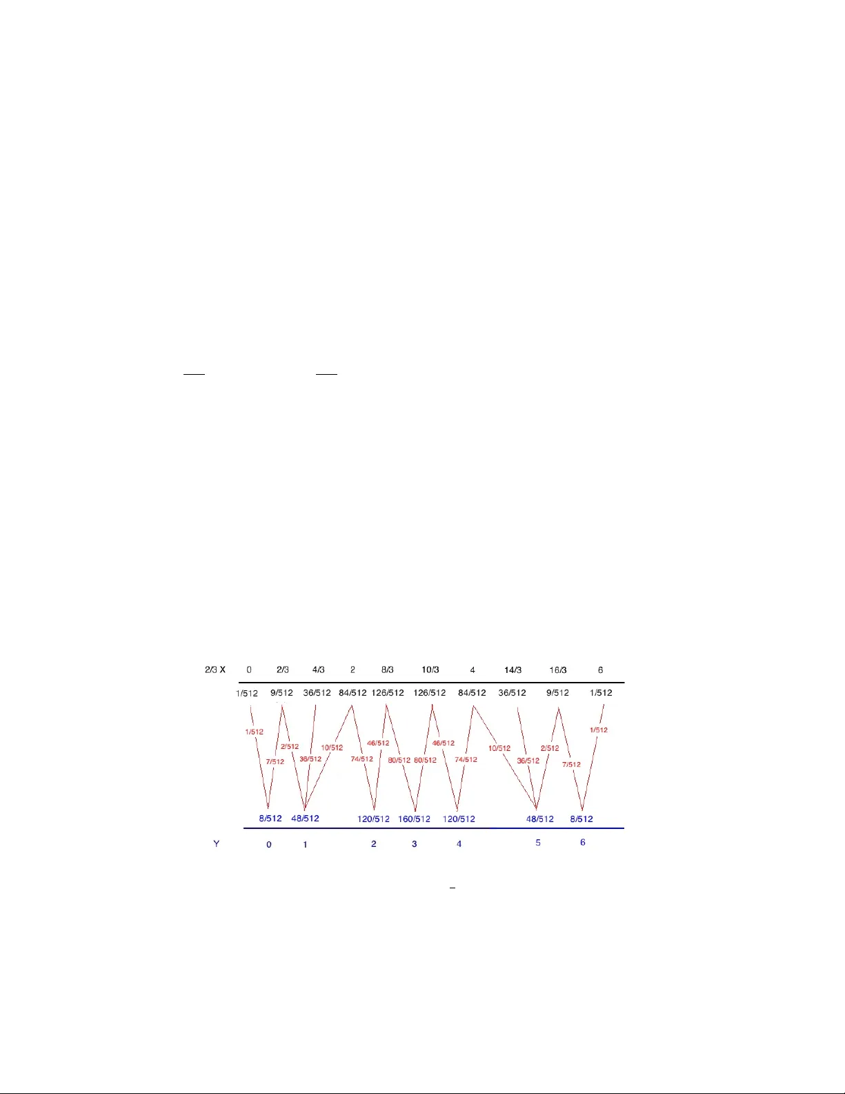
THE POISSON BINOMIAL DISTRIBUTION – OLD & NEW WENPIN T ANG AND FENGMIN T ANG Abstract. This is an exp ository article on the P oisson binomial distribution. W e review lesser kno wn results and recen t progress on this topic, including geometry of polynomials and distribution learning. W e also provide examples to illustrate the use of the Poisson binomial mac hinery . Some open questions of appro ximating rational fractions of the P oisson binomial are presen ted. Key wor ds : Distribution learning, geometry of p olynomials, P oisson binomial distribution, P oisson/normal appro ximation, optimal transport, sto c hastic ordering, strongly Ra yleigh prop ert y . 1. Introduction The binomial distribution is one of the earliest examples a college student encoun ters in his/her first course in probabilit y . It is a discrete probabilit y distribution of a sum of indep enden t and iden tically distributed (i.i.d.) Bernoulli random v ariables, mo deling the n um ber of o ccurrence of some ev en ts in rep eated trials. An integer-v alued random v ariable X is called binomial with parameters ( n, p ), denoted as X ∼ Bin( n, p ), if P ( X = k ) =  n k  p k (1 − p ) n − k , 0 ≤ k ≤ n . It is w ell known that if n is large, the Bin( n, p ) distribution is appro ximated by the P oisson distribution for small p ’s, and is appro ximated by the normal distribution for larger v alues of p . See e.g. [77] for an educational tour. P oisson [81] considered a more general mo del of indep endent trials, which allo ws hetero- geneit y among these trials. Precisely , an in teger-v alued random v ariable X is called Poisson binomial, and denoted as X ∼ PB( p 1 , . . . , p n ) if X ( d ) = ξ 1 + · · · + ξ n , where ξ 1 , . . . , ξ n are indep enden t Bernoulli random v ariables with parameters p 1 , . . . , p n . It is easily seen that the probabilit y distribution of X is P ( X = k ) = X A ∈ [ n ] , | A | = k Y i ∈ A p i Y i / ∈ A (1 − p i ) ! , (1.1) where the sum ranges o v er all subset of [ n ] := { 1 , . . . , n } of size k . The Poisson binomial distribution has a v ariety of applications such as reliability analysis [16, 57], surv ey sampling [29, 104], finance [40, 92], and engineering [44, 100]. Though this topic has b een studied for a long time, the literature is scattered. F or instance, the Poisson binomial distribution has differen t names in v arious con texts: P´ oly a frequency (PF) distribu- tion, strongly Ra yleigh distribution, con v olutions of heterogenous Bernoulli, etc. Researc hers often w ork on some asp ects of this sub ject, and ignore its connections to other fields. In late Date : August 28, 2019. 1 2 WENPIN T ANG AND FENGMIN T ANG 90’s, Pitman [78] wrote a surv ey on the Poisson binomial distribution with fo cus on probabi- lizing combinatorial sequences. Due to its applications in mo dern technology (e.g. mac hine learning [25, 89], causal inference (Example 3.4)) and links to different mathematical fields (e.g. algebraic geometry , mathematical physics), w e are motiv ated to surv ey recent studies on the Poisson binomial distribution. While most results in this pap er are known in some form, sev eral pieces are new (e.g. Section 4). The aim of this pap er is to provide a guide to lesser kno wn results and recent progress of the Poisson binomial distribution, mostly p ost 2000. The rest of the paper is organized as follows. In Section 2, we review distributional prop er- ties of the P oisson binomial distribution. In Section 3, v arious appro ximations of the Poisson binomial distribution are presen ted. Section 4 is concerned with the Poisson binomial dis- tribution and p olynomials with nonnegative co efficients. There w e discuss the problem of appro ximating rational fractions of Poisson binomial. Finally in Section 5, we consider some computational problems related to the P oisson binomial distribution. 2. Distributional proper ties of Poisson binomial v ariables In this section, we review a few distributional prop erties of the Poisson binomial distribu- tion. F or X ∼ PB( p 1 , . . . , p n ), w e hav e µ := E X = n ¯ p and σ 2 := V ar X = n ¯ p (1 − ¯ p ) − n X i =1 ( p i − ¯ p ) 2 , (2.1) where ¯ p := P n i =1 p i /n . It is easily seen that b y k eeping E X (or ¯ p ) fixed, the v ariance of X is increasing as the set of probabilities { p 1 , . . . , p n } gets more homogeneous, and is maximized as p 1 = · · · = p n . There is a simple in terpretation in survey sampling: taking samples from differen t comm unities ( str atifie d sampling ) is b etter than taking from the same group ( simple r andom sampling ). The abov e observ ation motiv ates the study of sto chastic orderings for the P oisson binomial distribution. The first result of this kind is due to Ho effding [53], claiming that among all P oisson binomial distributions with a giv en mean, the binomial distribution is the most spread-out. Theorem 2.1. [53] (Ho effding’s ine qualities) L et X ∼ PB( p 1 , . . . , p n ) , and ¯ X ∼ Bin( n, ¯ p ) . (1) Ther e ar e ine qualities P ( X ≤ k ) ≤ P ( ¯ X ≤ k ) for 0 ≤ k ≤ n ¯ p − 1 , and P ( X ≤ k ) ≥ P ( ¯ X ≤ k ) for n ¯ p ≤ k ≤ n. (2) F or any c onvex function g : [ n ] → R in the sense that g ( k + 2) − 2 g ( k + 1) + g ( k ) > 0 , 0 ≤ k ≤ n − 2 , we have E g ( X ) ≤ E g ( ¯ X ) , wher e the e quality holds if and only if p 1 = · · · = p n = ¯ p . The part (2) in Theorem 2.1 indicates that among all P oisson binomial distributions, the binomial is the largest one in con v ex order. This result w as extended to the multidimensional POISSON BINOMIAL 3 setting [9], and to non-negative random v ariables [8, Prop osition 3.2]. See also [68] for in terpretations. Next w e give several applications of Ho effding’s inequalities. Examples 2.2. (1) Monotonicity of binomials. Fix λ > 0. By taking ( p 1 , . . . , p n ) = (0 , λ n − 1 , . . . , λ n − 1 ), w e get for X ∼ Bin( n − 1 , λ n − 1 ) and X 0 ∼ Bin( n, λ n ), P ( X ≤ k ) < P ( X 0 ≤ k ) for k ≤ λ − 1 and P ( X ≤ k ) > P ( X 0 ≤ k ) for k ≥ λ. Similarly , by taking ( p 1 , . . . , p n ) = (1 , λ − 1 n − 1 , . . . , λ − 1 n − 1 ), w e get for X ∼ Bin( n − 1 , λ − 1 n − 1 ) and X 0 ∼ Bin( n, λ n ), P ( X ≤ k − 1) < P ( X 0 ≤ k ) for k ≤ λ − 1 and P ( X ≤ k − 1) > P ( X 0 ≤ k ) for k ≥ λ. These inequalities w ere used in [3] to deriv e the monotonicit y of error in appro ximat- ing the binomial distribution b y a P oisson distribution. By letting X ∼ Bin( n, p ) and Y ∼ P oi ( np ), they pro v ed P ( X ≤ k ) − P ( Y ≤ k ) is p ositive if k ≤ n 2 p/ ( n + 1) and is negativ e if k ≥ np . The result quantifies the error of confidence lev els in h yp othesis testing when appro ximating the binomial distribution by a Poisson distribution. (2) Darr o ch’s rule. It is well kno wn that a P oisson binomial v ariable has either one, or tw o consecutiv e mo des. By an argumen t in the pro of of Ho effding’s inequalities, Darro c h [32, Theorem 4] sho w ed that the mode m of the P oisson binomial distribution differs from its mean µ b y at most 1. Precisely , he prov ed that m =    k if k ≤ µ < k + 1 k +2 , k or k + 1 if k + 1 k +2 ≤ µ ≤ k + 1 − 1 n − k +1 , k + 1 if k + 1 − 1 n − k +1 < µ ≤ k + 1 . (2.2) This result was repro v ed in [91]. See also [60] for a similar result concerning the median. (3) Azuma-Ho effding ine quality. By the Azuma-Ho effding inequalit y [5, 54], for ξ 1 , . . . , ξ n indep enden t random v ariables such that 0 ≤ ξ i ≤ 1, P n X i =1 ξ i ≥ t ! ≤  µ t  t  n − µ n − t  n − t for t > µ, (2.3) where µ := P n i =1 E ξ i . Now we sho w how to derive a v ersion of (2.3) via a Poisson binomial tric k. Giv en ξ 1 , . . . , ξ n , let b i b e indep endent Bernoulli with parameter ξ i and X ∼ Bin  n, 1 n P n i =1 ξ i  . W e hav e P n X i =1 b i ≥ t      n X i =1 ξ i ≥ t ! ≤ P ( P n i =1 b i ≥ t ) P ( P n i =1 ξ i ≥ t ) . (2.4) Giv en P n i =1 ξ i ≥ t , P n i =1 b i is Poisson binomial with mean greater than t . According to Ho effding’s inequality , P n X i =1 b i ≥ t      n X i =1 ξ i ≥ t ! ≥ P X ≥ t      n X i =1 ξ i ≥ t ! ≥ c, (2.5) for some universal constant c > 0. Combining (2.4) and (2.5) yields P ( P n i =1 ξ i ≥ t ) ≤ c P ( P n i =1 b i ≥ t ). Note that P n i =1 b i is Poisson binomial with mean µ . Applying 4 WENPIN T ANG AND FENGMIN T ANG Ho effding’s inequalit y to P n i =1 b i with b ounds for binomial tails [71], we get P n X i =1 b i ≥ t ! ≤  µ t  t  n − µ n − t  n − t for t ≥ µ + 1 . (2.6) As a consequence, P ( P n i =1 ξ i ≥ t ) ≤ c  µ t  t  n − µ n − t  n − t whic h ac hiev es the same rate as in (2.3) up to a constan t factor. The original pro of of Theorem 2.1 was brute-force, and it w as soon generalized by using the idea of majorization and Schur c onvexity . T o pro ceed further, we need some vocabularies. Let { x (1) , . . . , x ( n ) } b e the order statistics of { x 1 , . . . , x n } . Definition 2.3. The ve ctor x x x is said to majorize the ve ctor y y y , denote d as x x x  y y y , if k X i =1 x ( i ) ≤ k X i =1 y ( i ) for k ≤ n − 1 and n X i =1 x ( i ) = n X i =1 y ( i ) . See [66] for background and developmen t on the theory of ma jorization and its applications. The follo wing theorem gives a few lesser known v arian ts of Ho effding’s inequalities. Theorem 2.4. L et X ∼ PB( p 1 , . . . , p n ) , X 0 ∼ PB( p 0 1 , . . . , p 0 n ) and Y ∼ Bin( n, p ) . (1) [48, 104] If ( p 1 , . . . , p n )  ( p 0 1 , . . . , p 0 n ) , then P ( X ≤ k ) ≤ P ( X 0 ≤ k ) for 0 ≤ k ≤ n ¯ p − 2 , and P ( X ≤ k ) ≥ P ( X 0 ≤ k ) for n ¯ p + 2 ≤ k ≤ n. Mor e over, V ar( X ) ≤ V ar( X 0 ) . (2) [80] If ( − log p 1 , . . . , − log p n )  ( − log p 0 1 , . . . , − log p 0 n ) , then X is sto chastic al ly lar ger than X 0 , i.e. P ( X ≥ k ) ≤ P ( X 0 ≥ k ) for al l k . (3) [17] X is sto chastic al ly lar ger than Y if and only if p ≤ ( Q n i =1 p i ) 1 n , and X is sto chas- tic al ly smal ler than Y if and only if p ≥ 1 − ( Q n i =1 (1 − p i )) 1 n . Conse quently, if ( Q n i =1 p i ) 1 n ≥ 1 − ( Q n i =1 (1 − p 0 i )) 1 n then X is sto chastic al ly lar ger than X 0 . The pro of of Theorem 2.4 relies on the fact that x x x  y y y implies the comp onents of x x x are more spread-out than those of y y y . F or example in part (1), it b oils down to pro ving if k ≤ n ¯ p − 2, P ( X ≤ k ) is a Sch ur conca v e function in p p p , meaning its v alue increases as the comp onents of p p p are less disp ersed. The part (3) gives a sufficien t condition of sto c hastic orderings for the Poisson binomial distribution. A simple necessary and sufficient condition remains op en. See also [15, 16, 18, 52, 93, 107] for further results. 3. Appro xima tion of Poisson binomial distributions In this section, we discuss v arious approximations of the P oisson binomial distribution. Pitman [78, Section 2] ga v e an excellent survey on this topic in the mid-90’s. W e complemen t the discussion with recent dev elopmen ts. In the sequel, L ( X ) denotes the distribution of a random v ariable X . POISSON BINOMIAL 5 P oisson appro ximation . Le Cam [64] ga v e the first error b ound for P oisson appro ximation of the Poisson binomial distribution. The following theorem is an improv emen t of Le Cam’s b ound. Theorem 3.1. [7] L et X ∼ PB( p 1 , . . . , p n ) and µ := P n i =1 p i . Then 1 32 min  1 , 1 µ  n X i =1 p 2 i ≤ d T V ( L ( X ) , Poi( µ )) ≤ 1 − e − µ 2 µ n X i =1 p 2 i , (3.1) wher e d T V ( · , · ) is the total variation distanc e. It is easily seen from (3.1) that the Poisson approximation of the Poisson binomial is go o d if P n i =1 p 2 i  P n i =1 p i , or equiv alently µ − σ 2  µ . There are t w o cases: • F or small µ , the upp er b ound in (3.1) is sharp. • F or large µ , the approximation error is of order P n i =1 p 2 i / P n i =1 p i . As p oin ted out in [59], the constan t 1 / 32 in the low er b ound can b e impro v ed to 1 / 14. See [6] for a b o ok-length treatment, and [86] for sharp b ounds. A p ow erful to ol to study the appro ximation of the sum of (p ossibly dep enden t) random v ariables is Stein’s method of exc hangeable pairs, see [26]. F or instance, a simple pro of of the upp er b ound in (3.1) was giv en in [26, Section 3] via the Stein machinery . The Poisson approximation can b e view ed as a mean-matc hing pro cedure. The failure of the Poisson appro ximation is due to a lac k of control in v ariance. A typical example is where all p i ’s are b ounded aw a y from 0, so that µ is large and P n i =1 p 2 i / P n i =1 p i is of constant order. T o deal with these cases, R¨ ollin [85] prop osed a mean/v ariance-matching pro cedure. T o present further results, we need the follo wing definition. Definition 3.2. An inte ger-value d r andom variable X is said to b e tr anslate d Poisson dis- tribute d with p ar ameters ( µ, σ 2 ) , denote d as TP( µ, σ 2 ) , if X − µ + σ 2 + { µ − σ 2 } ∼ P oi( σ 2 + { µ − σ 2 } ) , wher e {·} is the fr action p art of a p ositive numb er. It is easy to see that a TP( µ, σ 2 ) random v ariable has mean µ , and v ariance σ 2 + { µ + σ 2 } whic h is b et w een σ 2 and σ 2 + 1. The following theorem giv es an upper b ound in total v ariation b et w een a Poisson binomial v ariable and its translated Poisson appro ximation. Theorem 3.3. [85] L et X ∼ PB( p 1 , . . . , p n ) , and µ := P n i =1 p i and σ 2 := P n i =1 p i (1 − p i ) . Then d T V ( L ( X ) , TP( µ, σ 2 )) ≤ 2 + q P n i =1 p 3 i (1 − p i ) σ 2 , (3.2) wher e d T V ( · , · ) is the total variation distanc e. Note that if all p i ’s are b ounded aw ay from 0 and 1, the approximation error is of order 1 / √ n which is optimal. See [70] for the most up-to-date results of the P oisson appro ximation. No w we give an application of translated Poisson approximation in observ ational studies. Example 3.4. Sensitivity analysis. In matched-pair observ ational studies, an sensitivity analysis accesses the sensitivit y of results to hidden bias. Here w e follo w a mo dern approac h of Rosen baum [88, Chapter 4]. Precisely , the sample consists of n matched pairs and units in each pair are indexed b y i = 1 , 2. Eac h pair k = 1 , . . . , n is matched on a set of observ ed co v ariates x x x k 1 = x x x k 2 , and only one unit in eac h pair receives the treatmen t. Let Z ki b e the 6 WENPIN T ANG AND FENGMIN T ANG treatmen t assignment, so Z k 1 + Z k 2 = 1. Common test statistics for matched pairs are sign- score statistics of the form: T = P n k =1 d k ( c k 1 Z k 1 + c k 2 Z k 2 ), where d k ≥ 0 and c ki ∈ { 0 , 1 } . F or simplicity , we tak e d k = 1 and the statistics of in terest are T = n X k =1 ( c k 1 Z k 1 + c k 2 Z k 2 ) , (3.3) where c k 1 Z k 1 + c k 2 Z k 2 is Bernoulli distributed with parameter p k := c k 1 π k + c k 2 (1 − π k ) with π k := P ( Z k 1 = 1 | Z k 1 + Z k 2 = 1). So T ∼ PB( p 1 , . . . , p n ). F or 1 ≤ k ≤ n , let Γ k := π k / (1 − π k ), whic h equals to 1 if there is no hidden bias. The goal is to make inference on T with different choices of ( π 1 , . . . , π n ) and understand whic h c hoices explain aw a y the conclusion we dra w from the null hypothesis (i.e. there is no hidden bias). Thus, w e are interested in the set R ( t, α ) := { ( π 1 , . . . , π n ) : P ( T ≥ t ) ≤ α } , on the boundary of which the conclusion assuming no hidden bias is turned ov er. Ho w ev er, direct computation of R ( t, α ) seems hard. A routine wa y to solve this problem is to ap- pro ximate R ( t, α ) by a regular shap e. T o this end, w e consider the following optimization problem: max Γ , s.t. max π π π ∈ C Γ P ( T ( π 1 , . . . , π n ) ≥ t ) ≤ α, (3.4) where C Γ is a constrain t region. F or instance, C Γ := { π π π : 1 1+Γ ≤ π k ≤ Γ 1+Γ } corresp onds to the worst-case sensitivity analysis. By the translated Poisson approximation, the quantit y max π π π ∈ C Γ P ( T ( π 1 , . . . , π n ) ≥ t ) can b e ev aluated by the following problem which is easy to solv e. min A ∈{ 0 ,...,K } min π π π ∈ C Γ K X k =0 λ k e − λ k ! s.t. K = t − A, λ = n X k =1 p k − A, A ≤ n X k =1 p 2 k < A + 1 . (3.5) Normal approximation . The normal approximation of the Poisson binomial distribution follo ws from Lyapuno v or Lindeb erg central limit theorem, see e.g. [11, Section 27]. Berry and Esseen indep endently disco v ered an error b ound in terms of the cum ulativ e distribu- tion function for the normal approximation of the sum of indep endent random v ariables. Subsequen t improv emen ts w ere obtained by [72, 75, 94, 102] via F ourier analysis, and by [27, 28, 67, 101] via Stein’s metho d. Let φ ( x ) := 1 √ 2 π exp  − x 2 / 2  b e the probability density function of the standard normal, and Φ( x ) := R x −∞ φ ( y ) dy b e its cumulativ e distribution function. The following thero em pro vides uniform b ounds for the normal approximation of Poisson binomial v ariables. Theorem 3.5. L et X ∼ PB( p 1 , . . . , p n ) , and µ := P n i =1 p n and σ 2 := P n i =1 p i (1 − p i ) . (1) [79, Theorem 11.2] Ther e is a universal c onstant C > 0 such that max 0 ≤ k ≤ n     P ( X = k ) − φ  k − µ σ      ≤ C σ . (3.6) POISSON BINOMIAL 7 (2) [94] We have max 0 ≤ k ≤ n     P ( X ≤ k ) − Φ  k − µ σ      ≤ 0 . 7915 σ . (3.7) Other than uniform b ounds (3.6)-(3.7), several authors [14, 49, 84] studied error b ounds for the normal appro ximation in other metrics. F or µ , ν t w o probability measures, consider • L p metric d p ( µ, ν ) :=  Z ∞ −∞ | µ ( −∞ , x ] − ν ( −∞ , x ] | p dx  1 p , • W asserstein’s p metric W p ( µ, ν ) := inf π  Z ∞ −∞ Z ∞ −∞ | x − y | p π ( dxdy )  1 p , where the infim um runs ov er all probabilit y measures π on R × R with marginals µ and ν . Sp ecializing these b ounds to the Poisson binomial distribution, we get the follo wing result. Theorem 3.6. L et X ∼ PB( p 1 , . . . , p n ) , and µ := P n i =1 p n and σ 2 := P n i =1 p i (1 − p i ) . (1) [76, Chapter V] Ther e exists a universal c onstant C > 0 such that d p ( L ( X ) , N ( µ, σ 2 )) ≤ C σ for al l p ≥ 1 . (3.8) (2) [14, 84] F or e ach p ≥ 1 , ther e exists a c onstant C p > 0 such that W p ( L ( X ) , N ( µ, σ 2 )) ≤ C p σ . (3.9) Goldstein [49] pro v ed L p b ound (3.8) for p = 1 with C = 1. The general case follows from the inequality d p ( µ, ν ) p ≤ d ∞ ( µ, ν ) p − 1 d 1 ( µ, ν ) together with Goldstein’s L 1 b ound and the uniform b ound (3.7). By the Kantoro vic h-Rubinstein duality , d 1 ( µ, ν ) = W 1 ( µ, ν ). So the b ound (3.9) holds for p = 1 with C 1 = 1. F or general p , the b ound (3.9) is a consequence of the fact that for Z = P n i =1 ξ i with ξ i ’s indep enden t, E ξ i = 0 and P n i =1 V ar( ξ i ) = 1, W p ( L ( Z ) , N (0 , 1)) ≤ C p n X i =1 E | Z i | p +1 ! 1 p . This result w as prov ed in [84] for 1 ≤ p ≤ 2, and generalized to all p ≥ 1 in [14]. Binomial approximation . The binomial approximation of the P oisson binomial is lesser kno wn. The first result of this kind is due to Ehm [41] who prov ed that for X ∼ PB( p 1 , . . . , p n ), d T V ( L ( X ) , Bin( n, µ/n )) ≤ 1 − ( µ/n ) n +1 − (1 − µ/n ) n +1 ( n + 1)(1 − µ/n ) µ/n n X i =1 ( p i − µ/n ) 2 . (3.10) Elm’s approach w as extended to a Kra wtc houk expansion in [87]. The adv antage of the binomial appro ximation o v er the Poisson approximation is justified by the follo wing result due to Choi and Xia [31]. 8 WENPIN T ANG AND FENGMIN T ANG Theorem 3.7. L et X ∼ PB( p 1 , . . . , p n ) , and µ := P n i =1 p n . F or m ≥ 1 , let d m := d T V ( L ( X ) , Bin( m, µ/m )) . Then for m sufficiently lar ge, d m < d m +1 < · · · < d T V ( L ( X ) , Poi( µ )) . (3.11) See also [6, 73] for multi-parameter binomial appro ximations, and [95] for the P´ oly a approx- imation of the P oisson binomial distribution. 4. Poisson binomial distributions, pol ynomials with nonnega tive coefficients and optimal transpor t In this section, we discuss asp ects of the Poisson binomial distribution related to p oly- nomials with nonnegative co efficients. F or X ∼ PB( p 1 , . . . , p n ), the probability generating function (PGF) of X is f ( u ) := E X u = n Y i =1 ( p i u + 1 − p i ) . (4.1) It is easy to see that f is a p olynomial with all nonnegative co efficien ts, and all of its ro ots are real negative. The story starts with the following remark able theorem, due to Aissen, Endrei, Sc ho en b erg and Whitney [1, 2]. Theorem 4.1. [1, 2] L et ( a 0 , . . . , a n ) b e a se quenc e of nonne gative r e al numb ers, with asso- ciate d gener ating p olynomial f ( z ) := P n i =0 a i z i . The fol lowing c onditions ar e e quivalent: (1) The p olynomial f ( z ) has only r e al r o ots. (2) The se quenc e ( a 0 /f (1) , . . . , a n /f (1)) is the pr ob ability distribution of a PB( p 1 , . . . , p n ) distribution for some p i . The r e al r o ots of f ( z ) ar e − (1 − p i ) /p i for i with p i > 0 . (3) The se quenc e ( a 0 , . . . , a n ) is a P´ olya fr e quency (PF) se quenc e, i.e. the T o eplitz matrix ( a j − i ) i,j is total ly nonne gative. See [4] for bac kground on total p ositivity . F rom a computational asp ect, the condition (3) amoun ts to solving a system of n ( n − 1) / 2 p olynomial inequalities [42, 46]. Theorem 4.1 justifies the alternative name ‘PF distribution’ for the Poisson binomial distribution. Stan- dard references for PF sequences are [22, 96]. See also [78] for probabilistic interpretations for p olynomials with only negativ e real ro ots, and [55] for v arious extensions of Theorem 4.1 b y linear algebra. A p olynomial is called stable if it has no ro ots with p ositiv e imaginary part, and a stable p olynomial with all real co efficien ts is called real stable [19, 20]. In [21], a discrete distribution is said to b e strongly Rayleigh if its PGF is real stable. It w as also shown that the strong Ra yleigh prop ert y enjoys all virtues of negative dep endence. The follo wing result is a simple consequence of Theorem 4.1. Corollary 4.2. A r andom variable X ∼ PB( p 1 , . . . , p n ) for some p i if and only if X is str ongly R ayleigh on { 0 , . . . , n } . In the sequel, we use the terminologies ‘Poisson binomial’ and ‘strongly Ra yleigh’ in ter- c hangeably . Call a p olynomial f ( z ) = P n i =0 a i z i with a i ≥ 0 strongly Ra yleigh if it satisfies one of the conditions in Theorem 4.1. POISSON BINOMIAL 9 F or n ≥ 5, it is hop eless to get any ‘simple’ necessary and sufficient condition for f to b e strongly Ra yleigh due to Ab el’s imp ossibilit y theorem. A necessary condition for f to b e strong Ra yleigh is the Newton’s inequality: a 2 i ≥ a i − 1 a i +1  1 + 1 i   1 + 1 n − i  , 1 ≤ i ≤ n − 2 , (4.2) The sequence ( a i ; 0 ≤ i ≤ n ) satisfying (4.2) is also said to b e ultra-logconca ve [74]. Conse- quen tly , ( a i ; 0 ≤ i ≤ n ) is logconcav e and unimo dal. A lesser kno wn sufficient condition is giv en in [58, 63]: a 2 i > 4 a i − 1 a i +1 . 1 ≤ i ≤ n − 2 . (4.3) See also [50, 61] for v arious generalizations. As observed in [62], the inequalit y (4.3) cannot be impro ved since the sequence ( m i ; i ≥ 0) defined b y m i := inf n a 2 i a i − 1 a i +1 ; f is strong Ra yleigh o decreases from m 1 = 4 to its limit appro ximately 3 . 2336. In recen t w ork [47], the authors considered the multiv ariate CL T from strongly Rayleigh prop ert y . They raised the follo wing question: if X is a strong Rayleigh, or Poisson binomial random v ariable, how w ell can one approximate j X/k for eac h j, k ≥ 1 by a strong Ra yleigh, or Poisson binomial random v ariable ? A go o d approximation combined with the Cr´ amer- W old device prov es the CL T for multiv ariate strongly Rayleigh v ariables. The case j = 1 w as solved in that pap er. Theorem 4.3. [47] L et X b e a str ongly R ayleigh r andom variable. Then  X k  is str ongly R ayleigh for e ach k ≥ 1 , wher e b x c is the inte ger p art of x . The key to the pro of of Theorem 4.3 is [47, Theorem 4.3]: F or f a p olynomial of degree n and k ≥ 1, write f ( z ) = P k − 1 j =0 x j g j ( z k ), with g j a p olynomial of degree b n − j k c . The theorem asserts that if f is strongly Rayleigh, then so are g i ’s with in terlacing ro ots. In fact, the real-ro otedness follo ws from the fact that ( a n ; n ≥ 0) is a P´ olya frequency sequence = ⇒ ( a kn + j ; n ≥ 0) is a P´ olya frequency sequence , for each k ≥ 1 and 0 ≤ j < k . This result is well kno wn, see [1, Theorem 7] or [22, Theorem 3.5.4]. But the ro ot interlacing seems less obvious b y P´ oly a frequency sequences. A natural question is whether b j X/k c is strongly Ra yleigh for eac h j, k ≥ 1. It turns out that b 2 X/ 3 c can b e far aw ay from b eing strongly Rayleigh. In fact, one can prov e the follo wing theorem. Theorem 4.4. L et X ∼ Bin(3 n, 1 / 2) , and z i b e the r o ots of the pr ob ability gener ating func- tion of b 2 X/ 3 c . Then max i {= ( z i ) } ≥ r 9 n 2 − 9 n − 1 2 , (4.4) wher e = ( z ) is the imaginary p art of z . The reason why some ro ots of the PGF of b 2 X/ 3 c hav e large p ositiv e imaginary parts is due to the un balanced allo cation of probabilit y w eigh ts to ev en and o dd n umbers: P  2 X 3  = 2 k  =  3 n +1 3 k +1  while P  2 X 3  = 2 k + 1  =  3 n 3 k +2  . So the Newton’s inequality (4.2) is not satisfied. 10 WENPIN T ANG AND FENGMIN T ANG Optimal transp ort . F or simplicity , w e consider X ∼ Bin(3 n, 1 / 2). The goal is to find a coupling Y which is strongly Rayleigh on { 0 , 1 , . . . , 2 n } such that sup | Y − 2 X/ 3 | is as small as p ossible. Now w e provide a formulation of this problem via optimal transp ort. F or µ , ν t wo probability measures, define W ∞ ( µ, ν ) := inf γ ∈ π ( µ,ν ) { γ − ess sup | x − y |} , (4.5) where π ( µ, ν ) is the set of couplings of µ and ν . The metric W ∞ ( · , · ) is known as the ∞ - W asserstein distance, see [103]. A coupling γ whic h ac hieves the infim um (4.5) is called an optimal transference plan. By abuse of notation, write W ∞ ( X , Y ) for X ∼ µ , Y ∼ ν . W e w ant to solve the following optimization problem: Acc  2 X 3  := inf  W ∞  2 X 3 , Y  ; Y is strongly Rayleigh on { 0 , 1 , . . . , 2 n }  . (4.6) Here Acc(2 X/ 3) stands for the accuracy of strongly Ra yleigh ap pro ximations to 2 X/ 3. So the smaller the v alue of Acc(2 X/ 3) is, the better the appro ximation is. In [47], it w as conjectured that Acc(2 X/ 3) = O (1). The problem (4.6) can b e divided into tw o stages: (1) Given the distribution of Y , find an optimal transference plan Y = φ (2 X/ 3) with p ossibly random φ . This is the Monge(-Kantoro vic h) problem. (2) Find Y among all strongly Rayleigh distributions on { 0 , 1 , . . . , 2 n } whic h ac hiev es the infim um of W ∞ (2 X/ 3 , Y ). It migh t b e difficult to solve the problem (4.6) explicitly , but one can obtain a go o d upp er b ound b y constructing a suitable transference plan. F or example, the transference plan b elow sho ws that for X ∼ Bin(9 , 1 / 2), the v ariable 2 X/ 3 can b e approximated by Y ∼ Bin(6 , 1 / 2) with W ∞ (2 X/ 3 , Y ) ≤ 1. This implies that Acc (2 X/ 3) ≤ 1 for X ∼ Bin(9 , 1 / 2). In Appendix A, w e compute Acc(2 X/ 3) with X ∼ Bin( n, 1 / 2) for small n ’s. Figure 1. A transference plan from 2 3 Bin(9 , 1 / 2) to Bin(6 , 1 / 2). In the part (1) of the program, one question is how well a Bin(2 n, p ) random v ariable for an y p can approximate 2 X/ 3. Unfortunately , the approximation is not so go o d as prov ed in the follo wing prop osition. POISSON BINOMIAL 11 Prop osition 4.5. L et X ∼ Bin(3 n, 1 / 2) , and Y ∼ Bin(2 n, p ) for 0 ≤ p ≤ 1 . Then ther e exists C p > 0 such that W ∞  2 X 3 , Y  ≥ C p n for lar ge n. (4.7) Pr o of. The extreme cases p = 0 , 1 are straightforw ard. Assume that 0 < p < 1. Consider transfer from 2 X/ 3 to { Y = 0 } with probability mass (1 − p ) 2 n . By definition of W ∞ , W ∞  2 X 3 , Y  ≥ inf ( k ; (1 − p ) 2 n ≤ 1 2 3 n k X i =0  3 n i  ) . It is well kno wn that for any λ < 1 / 2, P 3 λn i = o  3 n i  = 2 3 nH ( λ )+ o ( n ) , where H ( λ ) := − λ log 2 ( λ ) − (1 − λ ) log 2 (1 − λ ). It follows from standard analysis that for p < 1 − 1 / √ 8, W ∞  2 X 3 , Y  ≥ 3 λ p n , where λ p is the unique solution on [0 , 1 / 2) to the equation H ( λ ) = 2 3 log 2 (1 − p ) + 1. Similarly by considering transfer from 2 X/ 3 to { Y = 2 n } with probability mass p 2 n , we get for p > 1 / √ 8, W ∞  2 X 3 , Y  ≥ 3 λ p n , where λ p is the unique solution on [0 , 1 / 2) to the equation H ( λ ) = 2 3 log 2 ( p ) + 1. W e take C p to b e 3 λ p for p ≥ 1 / 2, and 3 λ p for p < 1 / 2.  The problem requires finding ( p 1 , . . . , p 2 n ) ∈ [0 , 1] 2 n suc h that W ∞ (2 X/ 3 , PB( p 1 , . . . , p n )) is small. By Prop osition 4.5, the v alues of p 1 , . . . , p 2 n cannot b e all to o small or to o large. Precisely , there exist i ∈ [2 n ] such that p i > 1 / √ 8, and j ∈ [2 n ] such that p j < 1 − 1 / √ 8. This suggests to consider the equidistributed sequence p i = i 2 n +1 for i ∈ [2 n ]. By letting Y ∼ PB(1 / (2 n + 1) , . . . , 2 n/ (2 n + 1)), we get E (2 X/ 3) = E Y = 2 n and V ar  2 3 X  ∼ V ar Y ∼ n/ 3. A similar argumen t as in Prop osition 4.5 shows that W ∞  2 3 X , Y  ≥ inf ( k ; 2 n Y i =1 i 2 n + 1 ≤ P k i =1  3 n i  2 3 n ) ≥ inf ( k ;  8 e 2  n ≤ k X i =1  3 n i  ) = 3 λ eq n, where λ eq ≈ 0 . 0041 is the unique solution on [0 , 1 / 2) to the equation H ( λ ) = 1 − 2 3 log 2 ( e ). Still the appro ximation is not go o d, but m uch b etter than the Bin(2 n, p ) approximation. Op en problem 4.6. Is ther e a r andom variable Y ∼ PB( p 1 , . . . , p n ) such that W ∞ (2 X/ 3 , Y ) is of or der o ( n ) ? What is the lower b ound of Acc(2 X/ 3) ? Co efficien ts of Poisson binomial PGF . F or simplicit y , w e tak e X ∼ Bin(3 n − 1 , 1 / 2). As men tioned, the most ob vious approximation b 2 X/ 3 c do es not satisfy the Newton’s inequalit y . It is in teresting to ask the following: can w e find ( a 0 , . . . , a 2 n − 1 ) ∈ R 2 n + suc h that a 2 k + a 2 k +1 =  3 n − 1 3 k  +  3 n − 1 3 k + 1  +  3 n − 1 3 k + 2  for k ∈ [ n − 1] , (4.8) and the p olynomial P ( x ) := P 2 n − 1 k =1 a k x k has all real ro ots ? If we are able to find such ( a 0 , . . . , a 2 n − 1 ), then Acc(2 X/ 3) ≤ 2 / 3 whic h is a desired result. Note that the sequence ( a 0 , . . . , a 2 n − 1 ) must satisfy the Newton’s inequality and th us is unimo dal. See also [90] for higher order Newton’s inequalities. 12 WENPIN T ANG AND FENGMIN T ANG According to (4.8), a 0 + a 1 = Θ( n 2 ), meaning that a 0 + a 1 ∼ C n 2 for some C > 0. If a 0 = Θ( n 2 ), then the condition a 2 1 ≥ a 0 a 2 implies that a 2 = O ( n 2 ). F urther the condition a 2 2 ≥ a 1 a 3 giv es that a 3 = O ( n 2 ). Consequently , a 2 + a 3 = O ( n 2 ) which contradicts the fact that a 2 + a 3 = Θ( n 5 ). So w e hav e a 1 = o ( n ) and a 2 = Θ( n 2 ). A similar argument sho ws that for any fixed k , a 2 k = o ( n 3 k +2 ) and a 2 k +1 = Θ( n 3 k +2 ). It can b e sho wn that a k = Θ( n 1+3 k 2 ) for any fixed k . But the choice for the bulk terms such as a n − 1 , a n is a more subtle issue since the terms  3 n b 3 n/ 2 c− 1  ,  3 n b 3 n/ 2 c  and  3 n b 3 n/ 2 c +1  are comparable. In App endix A, w e see that Acc(2 X/ 3) = 1 / 3 for n = 1, and Acc(2 X/ 3) = 2 / 3 for n = 2. F urther we get, • n = 3: Acc(2 X/ 3) = 2 / 3, achiev ed by a strongly Ra yleigh v ariable with PGF 1 2 8 (3 + 34 x + 91 x 2 + 91 x 3 + 34 x 4 + 3 x 5 ) . • n = 4: Acc(2 X/ 3) = 2 / 3, achiev ed by a strongly Ra yleigh v ariable with PGF 1 2 11 (4 + 63 x + 310 x 2 + 647 x 3 + 647 x 4 + 310 x 5 + 63 x 6 + 4 x 7 ) . • n = 5: Acc(2 X/ 3) = 2 / 3, achiev ed by a strongly Ra yleigh v ariable with PGF 1 2 14 (4 + 102 x + 760 . 5 x 2 + 2606 . 5 x 3 + 4719 x 4 + 4719 x 5 + 2606 . 5 x 6 + 760 . 5 x 7 + 102 x 8 + 4 x 9 ) . F rom small n cases, w e sp eculate there is a strongly Ra yleigh p olynomial P ( x ) whose co efficien ts satisfy (4.8) and the symmetric/self-recipro cal condition: a k = a 2 n − 1 − k for k ∈ [ n − 1] . (4.9) Suc h p olynomials are instances of Λ -p olynomials [23], whose co efficients are symmetric and unimo dal. In general, for each n ≥ 2 there exist a set of at most n − 1 p olynomials Q k ∈ Z [ a 0 , · · · , a n ] such that the p olynomial with real co efficien ts P ( x ) has only real ro ots if and only if Q k ≥ 0 for each k . These Q k ’s can b e constructed as the leading co efficien ts of the Sturm’s sequence of P , see e.g. [99, Section 1.3]. They are also the subresultan ts of the Sylv ester matrix of P and P 0 up to sign changes. In other words, we try to find whether the set S := { ( a 0 , . . . , a 2 n − 1 ) ∈ R + : (4.8) , (4.9) hold and Q k ≥ 0 for all k } is empty or not. The set S is semi-algebraic. According to Stengle’s P ositivstellensatz [98], the non-emptiness of S is equiv alent to − 1 / ∈ C ( Q 1 , . . . , Q n − 1 )+ I  a 2 k + a 2 k +1 −  3 n − 1 3 k  −  3 n − 1 3 k + 1  −  3 n − 1 3 k + 2  , a k − a 2 n − 1 − k  , where C is the cone and I is the ideal. Ho wev er, the size of the p olynomials Q k gro ws v ery fast, and hence exact computations b ecome imp ossible. See also [69, 83] for related discussions. Hurwitz stability . Recently , Liggett [65] pro v ed an in teresting result of b 2 X/ 3 c for X a strongly Ra yleigh v ariable. Theorem 4.7. [65] L et X b e a str ongly R ayleigh r andom variable. Then the PGF of b 2 X/ 3 c is Hurwitz stable. That is, al l its r o ots have ne gative r e al p arts. POISSON BINOMIAL 13 The idea is to write the PGF of b 2 X/ 3 c as g 0 ( x 2 ) + xg 1 ( x 2 ), where g 0 and g 1 ha ve in terlacing ro ots. By the Hermite-Biehler theorem [10, 51], such p olynomials are Hurwitz stable. This means that the PGF of b 2 X/ 3 c can b e factorized into p olynomials with p ositiv e co efficien ts of degrees no greater than 2. Th us, b 2 X/ 3 c is a Poisson multinomial v ariable, that is the sum of indep endent random v ariables with v alues in { 0 , 1 , 2 } . In general, it can b e shown that b j X/k c is expressed as g 0 ( x j ) + xg 1 ( x j ) + · · · + x j − 1 g j − 1 ( x j ) , (4.10) where g 0 . . . g j − 1 ha ve simple interlacing ro ots. W e conjecture the following. Conjecture 4.8. L et X b e a str ong R ayleigh r andom variable. Then b j X/k c is the sum of indep endent r andom variables with values in { 0 , 1 , . . . , j } . Equivalently, the PGF of b j X/k c c an b e factorize d into p olynomials with p ositive c o efficients of de gr e es no gr e ater than j . Let P j b e the set of p olynomials with p ositive co efficients which can b e factorized into p olynomials with p ositiv e co efficients of degrees no greater than j , and Q j b e the set of p olynomials which satisfies (4.10). F rom the ab ov e discussion, P 1 = Q 1 and P 2 = Q 2 . But neither implication b et w een P 3 and Q 3 is true, as the follo wing examples in [65] show: • Let f ( z ) = z 5 + z 4 + z 3 + 2 z 2 + 3 2 z + 1 3 . The roots of f are z 1 , ¯ z 1 , z 2 , ¯ z 2 and w with v alues z 1 = 0 . 725 + 0 . 100 i , z 2 = 0 . 435 + 1 . 137 i and w = 0 . 420. W e hav e ( z − z 2 )( z − ¯ z 2 )( z − w ) = 0 . 623 + 1 . 116 z − 0 . 449 z 2 + z 3 , so f / ∈ P 3 . But the ro ots of h 0 , h 1 , h 2 are − 1 3 , − 3 2 , − 2 resp ectiv ely , so f ∈ Q 3 . • Let f ( z ) = (1 + z + 2 z 2 )(25 + z 2 + 2 z 3 ) = 25 + 25 z + 51 z 2 + 3 z 3 + 4 z 4 + 4 z 5 , whic h is in P 3 , Ho wev er, f / ∈ Q 3 since the ro ots of h 0 , h 1 , h 2 are − 25 3 , − 25 4 , − 51 4 resp ectiv ely . See also [24, 106, 108] for discussion of p ositive factorizations of small degree p olynomials. 5. Comput a tions of Poisson binomial distributions In this section we discuss a few computational issues of learning and computing the P oisson binomial distribution. Learning the Poisson binomial distribution . Distribution learning is an active domain in b oth statistics and computer science. F ollo wing [36], given access to indep endent samples from an unkno wn distribution P , an error con trol  > 0 and a confidence level δ > 0, a learning algorithm outputs an estimation b P such that P ( d T V ( b P , P ) ≤  ) ≥ 1 − δ . The p erfor- mance of a learning algorithm is measured by its sample complexit y and its computational complexit y . F or X ∼ PB( p 1 , . . . , p n ), this amounts to finding a v ector ( b p 1 , . . . , b p n ) defining b X ∼ PB( b p 1 , . . . , b p n ) such that d T V ( b X , X ) is small with high probability . This is often called prop er learning of P oisson binomial distributions. Building up on previous work [12, 35, 85], Dask alakis, Diakonik olas and Serv edio [34] established the following result for prop er learning of P oisson binomial distributions. Theorem 5.1. [34] L et X ∼ PB( p 1 , . . . , p n ) with unknown p i ’s. Ther e is an algorithm such that given , δ > 0 , it r e quir es • (sample c omplexity) O (1 / 2 ) · log(1 /δ ) indep endent samples fr om X , • (c omputational c omplexity) (1 / ) O (log 2 (1 / )) · O (log n · log(1 /δ )) op er ations, 14 WENPIN T ANG AND FENGMIN T ANG to c onstruct a ve ctor ( b p 1 , . . . , b p n ) satisfying P ( d T V ( b X , X ) ≤  ) ≥ 1 − δ for b X ∼ PB( b p 1 , . . . , b p n ) . The key to the algorithm is to find subsets co vering all P oisson binomial distributions, and eac h of these subsets is either ‘sparse’ or ‘hea vy’. Applying Birg´ e’s algorithm [12] to sparse subsets, and the translated P oisson appro ximation (Theorem 3.3) to heavy subsets give the desired algorithm. Note that the sample complexity in Theorem 5.1 is nearly optimal, since Θ(1 / 2 ) samples are required to distinguish Bin( n, 1 / 2) from Bin( n, 1 / 2 + / √ n ) which differ b y Θ(  ) in total v ariation. See also [39] for further results on learning the P oisson binomial distribution, and [33, 37, 38] for the in teger-v alued distribution. Computing the P oisson binomial distri bution . Recall the probability distribution of X ∼ PB( p 1 , . . . , p n ) from (1.1). A brute-force computation of this distribution is exp ensiv e for large n . Approximations in Section 3 are often used to estimate the probability distribu- tion/CDF of the Poisson binomial distribution. Here we fo cus on the efficient algorithms to compute e xactly these distribution functions. There are tw o general approaches: recursive form ulas and discrete F ourier analysis. In [29], the authors presen ted several recursive algorithms to compute (1.1). F or B ⊂ [ n ], define R ( k , B ) := X A ⊂ B , | A | = k Y i ∈ A p i 1 − p i ! . So P ( X = k ) = R ( k , [ n ]) · Q n i =1 (1 − p i ). Now the problem is to find efficien t wa ys to compute R ( k , B ). Two recursive algorithms are prop osed: • [30, 97] F or B ⊂ [ n ], by letting T ( i, B ) := P j ∈ B  p j 1 − p j  i , R ( k , B ) = 1 k k X i =1 ( − 1) i +1 T ( i, B ) R ( k − i, B ) , (5.1) • [45] F or B ⊂ [ n ], R ( k , B ) = R ( k , B \ { k } ) + p k 1 − p k R ( k − 1 , B \ { k } ) . (5.2) In another direction, [43, 56] used a F ourier approac h to ev aluate the probability distribu- tion/CDF of P oisson binomial distributions. They provided the following explicit formulas: P ( X = k ) = 1 n + 1 n X j =0 exp( − iω k j ) x j , (5.3) and P ( X ≤ k ) = 1 n + 1 n X j =0 1 − exp( − iω ( k + 1) j ) 1 − exp( − iω j ) x j , (5.4) where ω := 2 π n +1 and x j := Q n k =1 (1 − p k + p k exp( iω j )). In particular, the r.h.s of (5.3) is the discrete F ourier transform of { x 0 , . . . , x n } which can b e easily computed by F ast F ourier T ransform. See also [13] for a related approach. POISSON BINOMIAL 15 Appendix A. Accura cy of 2 X/ 3 for small n Recall the definition of Acc( · ) from (4.6). W e compute the v alues of Acc(2 X/ 3) with X ∼ Bin( n, 1 / 2) for 1 ≤ n ≤ 6. • n = 1: Let Y ∼ Ber(1 / 2), where Ber( p ) is a Bernoulli v ariable with parameter p . It is easy to see that Acc(2 X/ 3) = W ∞ (2 X/ 3 , Y ) = 1 / 3 . That is, the weigh t P (2 X/ 3 = 0) = 1 / 2 is transferred to { Y = 0 } , and the weigh t P (2 X/ 3 = 2 / 3) = 1 / 2 is transferred to { Y = 1 } . • n = 2: Let Y ∼ Ber(3 / 4). W e hav e Acc(2 X/ 3) = W ∞ (2 X/ 3 , Y ) = 1 / 3 . So the w eight P (2 X/ 3 = 0) = 1 / 4 is transferred to { Y = 0 } , and the weigh t P (2 X/ 3 ∈ { 2 / 3 , 4 / 3 } ) = 3 / 4 is transferred to { Y = 1 } . • n = 3: supp ose that W ∞ (2 X/ 3 , Y ) = 1 / 3 for some integer-v alued v ariable Y . Then the weigh t P (2 X/ 3 = 0) = 1 / 8 is transferred to { Y = 0 } , the weigh t P (2 X/ 3 ∈ { 2 / 3 , 4 / 3 } ) = 3 / 4 is transferred to { Y = 1 } , and the weigh t P (2 X/ 3 = 2) = 1 / 8 is transferred to { Y = 2 } . The PGF of Y is 1 / 8 + 3 x/ 4 + x 2 / 8, which has tw o distinct real ro ots − 3 ± √ 8. Thus, Acc(2 X/ 3) = W ∞  2 X/ 3 , PB  1 4 + √ 8 , 1 4 − √ 8  = 1 / 3 . • n = 4: if W ∞ (2 X/ 3 , Y ) = 1 / 3 for some in teger-v alued Y , then the PGF of Y is 1 / 16 + 10 x/ 16 + 4 x 2 / 16 + x 3 / 16. This PGF has one real ro ot and tw o imaginary ro ots, so Y cannot b e strongly Rayleigh. There are many wa ys to construct a strongly Rayleigh v ariable Y suc h that W ∞ (2 X/ 3 , Y ) = 2 / 3. F or instance, the w eight P (2 X/ 3 = 0) = 1 / 16 is transferred to { Y = 0 } , the weigh t P (2 X/ 3 ∈ { 2 / 3 , 4 / 3 } ) = 10 / 16 is transferred to { Y = 1 } and the w eight P (2 X/ 3 ∈ { 2 , 8 / 3 } ) = 5 / 16 is transferred to { Y = 2 } . So Acc(2 X/ 3) = W ∞  2 X/ 3 , PB  1 2 + 2 / √ 5 , 1 2 − 2 / √ 5  = 2 / 3 . In fact, we can find all strongly Ra yleigh Y suc h that W ∞ (2 X/ 3 , Y ) = 2 / 3. There are t wo cases: (1) The range of Y is { 0 , 1 , 2 } . Supp ose θ 1 / 16 with θ 1 ≤ 4 of P (2 X/ 3 = 2 / 3) is transferred to { Y = 1 } , and θ 2 / 16 with θ 2 ≤ 6 of P (2 X/ 3 = 4 / 3) is transferred to { Y = 1 } . Then the PGF of Y is 5 − θ 1 16 + θ 1 + θ 2 16 x + 11 − θ 2 16 x 2 . So Y is strongly Rayleigh if and only if ( θ 1 + θ 2 ) 2 ≥ 4(5 − θ 1 )(11 − θ 2 ). Figure 2 (Left) sho ws the v alid region of ( θ 1 , θ 2 ). (2) The range of Y is { 0 , 1 , 2 , 3 } . Assume the same as in (1), and in addition θ 3 / 16 with θ 3 ≤ 1 of P (2 X/ 3 = 8 / 3) is transferred to { Y = 3 } . Then the PGF of Y is 5 − θ 1 16 + θ 1 + θ 2 16 x + 11 − θ 2 − θ 3 16 x 2 + θ 3 16 x 3 . 16 WENPIN T ANG AND FENGMIN T ANG The discriminant of the cubic equation ax 3 + bx 2 + cx + d = 0 is ∆ := 18 abcd − 4 b 3 d + b 2 c 2 − 4 ac 3 − 27 a 2 d 2 . According to a well kno wn result of Cardano, the cubic equation has three real ro ots if and only if ∆ ≥ 0 [105]. Sp ecializing to our case giv es 18(5 − θ 1 )( θ 1 + θ 2 )(11 − θ 2 − θ 3 ) θ 3 − 4(11 − θ 2 − θ 3 ) 3 (5 − θ 1 ) + (11 − θ 2 − θ 3 ) 2 ( θ 1 + θ 2 ) 2 − 4( θ 1 + θ 2 ) 3 θ 3 − 27(5 − θ 1 ) 2 θ 2 3 ≥ 0 . Figure 2 (Righ t) shows the v alid region of ( θ 1 , θ 2 , θ 3 ). Figure 2. Left: V alid region of ( θ 1 , θ 2 ). Right: V alid region of ( θ 1 , θ 2 , θ 3 ). • n = 5: a similar argumen t as in the case n = 4 sho ws that W ∞ (2 X/ 3 , Y ) 6 = 1 / 3 for each strongly Rayleigh v ariable Y . Again there are many w ays to construct a strongly Ra yleigh v ariable Y such that W ∞ (2 X/ 3 , Y ) = 2 / 3. F or instance, the w eight P (2 X/ 3 = 0) = 1 / 32 is transferred to { Y = 0 } , the weigh t P (2 X/ 3 ∈ { 2 / 3 , 4 / 3 } ) = 15 / 32 is transferred to { Y = 1 } , the w eight P (2 X/ 3 ∈ { 2 , 8 / 3 } ) = 15 / 32 is transferred to { Y = 2 } , and the weigh t P (2 X/ 3 = 10 / 3) = 1 / 32 is transferred to { Y = 3 } . The PGF of Y is then 1 / 32 + 15 x/ 32 + 15 x 2 / 32 + x 3 / 32. It is easily seen that the co efficien ts of the ab ov e PGF satisfy the Hutchinson-Kurtz condition (4.3). So Acc(2 X/ 3) = 2 / 3. It is more difficult to find all strongly Rayleigh v ariables Y suc h that W ∞ (2 X/ 3 , Y ) = 2 / 3, since the conditions for a quartic function to hav e all real ro ots are more complicated [82]. • n = 6: consider the transference plan in Figure 3. It is easy to see that the PGF of Y is 1 / 16(1 + x ) 4 , so Y ∼ Bin(4 , 1 / 2) and Acc(2 X/ 3) = 2 / 3. Ac knowledgmen t: W e thank T om Liggett, Jim Pitman and T erry T ao for helpful discus- sions. W e thank Y uting Y e for pro viding Example 3.4, and T om Liggett for showing us the man uscript [65]. References [1] M. Aissen, A. Edrei, I. J. Schoenberg, and A. Whitney . On the generating functions of totally p ositive sequences. Pr o c. Nat. Ac ad. Sci. U. S. A. , 37:303–307, 1951. [2] M. Aissen, I. J. Sc ho enberg, and A. Whitney . On the generating functions of totally p ositive sequences. I. J. Analyse Math. , 2:93–103, 1952. POISSON BINOMIAL 17 Figure 3. A transference plan from 2 3 Bin(6 , 1 / 2) to Bin(4 , 1 / 2). [3] T. W. Anderson and S. M. Samuels. Some inequalities among binomial and Poisson probabilities. In Pr o c. Fifth Berkeley Symp os. Math. Statist. and Pr obability (Berkeley, Calif., 1965/66) , pages V ol. I: Statistics, pp. 1–12. Univ. California Press, Berkeley , Calif., 1967. [4] T. Ando. T otally p ositive matrices. Line ar Algebr a Appl. , 90:165–219, 1987. [5] K. Azuma. W eighted sums of certain dep endent random v ariables. T ohoku Math. J. (2) , 19:357–367, 1967. [6] A. Barb our, L. Holst, and S. Janson. Poisson appro ximation. 1992. [7] A. D. Barb our and P . Hall. On the rate of Poisson conv ergence. Math. Pr o c. Cambridge Philos. So c. , 95(3):473–480, 1984. [8] D. Berend and T. T assa. Impro ved b ounds on Bell n umbers and on moments of sums of random v ariables. Pr ob ab. Math. Statist. , 30(2):185–205, 2010. [9] P . J. Bick el and W. R. v an Zwet. On a theorem of Ho effding. In Asymptotic the ory of statistic al tests and estimation (Pr o c. Adv. Internat. Sympos., Univ. North Car olina, Chap el Hil l, N.C., 1979) , pages 307–324. Academic Press, New Y ork-London-T oron to, Ont., 1980. [10] R. Biehler. Sur une classe d’´ equations alg´ ebriques dont toutes les racines sont r ´ eelles. J. R eine Angew. Math. , 87:350–352, 1879. [11] P . Billingsley . Pr ob ability and me asure . Wiley Series in Probabilit y and Mathematical Statistics. John Wiley & Sons, Inc., New Y ork, third edition, 1995. [12] L. Birg´ e. Estimation of unimo dal densities without smoothness assumptions. Ann. Statist. , 25(3):970– 981, 1997. [13] W. Biscarri, S. D. Zhao, and R. J. Brunner. A simple and fast metho d for computing the Poisson binomial distribution function. Comput. Statist. Data Anal. , 122:92–100, 2018. [14] S. G. Bobko v. Berry-Esseen b ounds and Edgew orth expansions in the cen tral limit theorem for transport distances. Pr ob ab. The ory R elated Fields , 170(1-2):229–262, 2018. [15] P . J. Boland. The probability distribution for the num b er of successes in indep endent trials. Comm. Statist. Theory Metho ds , 36(5-8):1327–1331, 2007. [16] P . J. Boland and F. Prosc han. The reliabilit y of k out of n systems. A nn. Prob ab. , 11(3):760–764, 1983. [17] P . J. Boland, H. Singh, and B. Cukic. Stochastic orders in partition and random testing of soft ware. J. Appl. Prob ab. , 39(3):555–565, 2002. [18] P . J. Boland, H. Singh, and B. Cukic. The stochastic precedence ordering with applications in sampling and testing. J. Appl. Pr ob ab. , 41(1):73–82, 2004. [19] J. Borcea and P . Br¨ and ´ en. Applications of stable p olynomials to mixed determinants: Johnson’s con- jectures, unimo dalit y , and symmetrized Fischer pro ducts. Duke Math. J. , 143(2):205–223, 2008. 18 WENPIN T ANG AND FENGMIN T ANG [20] J. Borcea and P . Br¨ and ´ en. P´ olya-Sc hur master theorems for circular domains and their b oundaries. A nn. of Math. (2) , 170(1):465–492, 2009. [21] J. Borcea, P .r Br¨ and´ en, and T. M. Liggett. Negative dep endence and the geometry of polynomials. J. Amer. Math. So c. , 22(2):521–567, 2009. [22] F. Brenti. Unimo dal, log-concav e and P´ olya frequency sequences in com binatorics. Mem. Amer. Math. So c. , 81(413):viii+106, 1989. [23] F. Brenti. Unimo dal p olynomials arising from symmetric functions. Pr oc. Amer. Math. So c. , 108(4):1133–1141, 1990. [24] W. E. Briggs. Zeros and factors of p olynomials with positive co efficients and protein-ligand binding. R o cky Mountain J. Math. , 15(1):75–89, 1985. [25] T. Bro deric k, J. Pitman, and M. I. Jordan. F eature allo cations, probability functions, and paintboxes. Bayesian Anal. , 8(4):801–836, 2013. [26] S. Chatterjee, P . Diaconis, and E. Meck es. Exchangeable pairs and Poisson approximation. Pr ob ab. Surv. , 2:64–106, 2005. [27] L. H. Y. Chen and Q-M Shao. A non-uniform Berry-Esseen bound via Stein’s metho d. Pr ob ab. The ory R elate d Fields , 120(2):236–254, 2001. [28] L. H. Y. Chen and Q-M Shao. Stein’s method for normal approximation. In An intr oduction to Stein ’s metho d , v olume 4 of L e ct. Notes Ser. Inst. Math. Sci. Natl. Univ. Singap. , pages 1–59. Singap ore Univ. Press, Singap ore, 2005. [29] S. X. Chen and J. S. Liu. Statistical applications of the Poisson-binomial and conditional Bernoulli distributions. Statist. Sinica , 7(4):875–892, 1997. [30] X-H Chen, A. P . Dempster, and J. S. Liu. W eighted finite p opulation sampling to maximize entrop y . Biometrika , 81(3):457–469, 1994. [31] K. P . Choi and A-H Xia. Approximating the n umber of successes in indep enden t trials: binomial v ersus Poisson. Ann. Appl. Prob ab. , 12(4):1139–1148, 2002. [32] J. N. Darro ch. On the distribution of the num b er of successes in independent trials. A nn. Math. Statist. , 35, 1964. [33] C. Dask alakis, I. Diak onikolas, R. O’Donnell, R. A. Servedio, and L-Y T an. Learning sums of indepen- den t in teger random v ariables. In F oundations of Computer Scienc e (FOCS), 2013 IEEE 54th Annual Symp osium , pages 217–226, 2013. [34] C. Dask alakis, I. Diakonik olas, and R. A. Servedio. Learning Poisson binomial distributions. Algorith- mic a , 72(1):316–357, 2015. [35] C. Dask alakis and C. P apadimitriou. Sparse co vers for sums of indicators. Pr ob ab. The ory Relate d Fields , 162(3-4):679–705, 2015. [36] L. Devroy e and G. Lugosi. Combinatorial metho ds in density estimation . Springer Series in Statistics. Springer-V erlag, New Y ork, 2001. [37] I. Diakonik olas, D. M. Kane, and A. Stewart. The Fourier transform of Poisson multinomial distribu- tions and its algorithmic applications. In STOC’16—Pr o c ee dings of the 48th Annual ACM SIGACT Symp osium on The ory of Computing , pages 1060–1073. ACM, New Y ork, 2016. [38] I. Diakonik olas, D. M. Kane, and A. Stewart. Optimal learning via the Fourier transform for sums of indep enden t in teger random v ariables. In Confer enc e on Le arning The ory , pages 831–849, 2016. [39] I. Diakonik olas, D. M. Kane, and A. Stewart. Properly learning Poisson binomial distributions in almost p olynomial time. In Confer enc e on Le arning The ory , pages 850–878, 2016. [40] D. Duffie, L. Saita, and K. W ang. Multi-perio d corp orate default prediction with stochastic cov ariates. Journal of Financial Ec onomics , 83(3):635–665, 2007. [41] W. Ehm. Binomial appro ximation to the Poisson binomial distribution. Statist. Pr ob ab. L ett. , 11(1):7–16, 1991. [42] S. F allat, C. R. Johnson, and A. D. Sok al. T otal p ositivit y of sums, Hadamard pro ducts and Hadamard p o w ers: results and counterexamples. Line ar Algebr a Appl. , 520:242–259, 2017. [43] M. F ern´ andez and S. Williams. Closed-form expression for the p oisson-binomial probability density function. IEEE T r ansactions on A er osp ac e and Ele ctronic Systems , 46(2):803–817, 2010. [44] M. F. F ernandez and T. Aridgides. Measures for ev aluating sea mine identification pro cessing p erfor- mance and the enhancemen ts provided by fusing multisensor/m ultipro cess data via an M-out-of-N v oting POISSON BINOMIAL 19 sc heme. In Dete ction and R emediation T e chnolo gies for Mines and Minelike T ar gets VIII , volume 5089, pages 425–436, 2003. [45] M. H. Gail, J. H. Lubin, and L. V. Rubinstein. Lik eliho o d calculations for matched case-control studies and surviv al studies with tied death times. Biometrika , 68(3):703–707, 1981. [46] M. Gasca and J. M. P e ˜ na. T otal p ositivit y and Neville elimination. Line ar Algebr a Appl. , 165:25–44, 1992. [47] S. Ghosh, T. M. Liggett, and R. P emantle. Multiv ariate CL T follo ws from strong Ra yleigh property . In 2017 Pr o c ee dings of the Fourte enth Workshop on Analytic Algorithmics and Combinatorics (ANALCO) , pages 139–147. SIAM, Philadelphia, P A, 2017. [48] L. J. Gleser. On the distribution of the n umber of successes in indep enden t trials. Ann. Pr ob a. , 3:182–188, 1975. [49] L. Goldstein. Bounds on the constant in the mean cen tral limit theorem. A nn. Pr ob ab. , 38(4):1672–1689, 2010. [50] D. Handelman. Argumen ts of zeros of highly log concav e p olynomials. R o cky Mountain J. Math. , 43(1):149–177, 2013. [51] C. Hermite. Sur le nombre des racines d’une ´ equation alg´ ebrique comprises entre des limites donn´ ees. J. Reine A ngew. Math. , 52:39–51, 1856. [52] E. Hillion and O. Johnson. A pro of of the Shepp-Olkin entrop y concavit y conjecture. Bernoul li , 23(4B):3638–3649, 2017. [53] W. Ho effding. On the distribution of the num b er of successes in indep endent trials. The Annals of Mathematic al Statistics , 27(3):713–721, 1956. [54] W. Ho effding. Probability inequalities for sums of b ounded random v ariables. J. Amer. Statist. Asso c. , 58:13–30, 1963. [55] O. Holtz and M. T yaglo v. Structured matrices, con tinued fractions, and ro ot localization of polynomials. SIAM Rev. , 54(3):421–509, 2012. [56] Y-L Hong. On computing the distribution function for the Poisson binomial distribution. Comput. Statist. Data Anal. , 59:41–51, 2013. [57] Y-L Hong, W. Q. Meeker, and J. D. McCalley . Prediction of remaining life of pow er transformers based on left truncated and right censored lifetime data. A nn. Appl. Stat. , 3(2):857–879, 2009. [58] J. I. Hutchinson. On a remark able class of entire functions. T r ans. A mer. Math. So c. , 25(3):325–332, 1923. [59] S. Janson. Coupling and Poisson approximation. A cta Appl. Math. , 34(1-2):7–15, 1994. [60] K. Jogdeo and S. M. Samuels. Monotone conv ergence of binomial probabilities and a generalization of Raman ujan’s equation. Ann. Math. Statist. , 39(4):1191–1195, 1968. [61] O. M. Katko v a and A. M. Vishny ako v a. A sufficient condition for a p olynomial to b e stable. J. Math. Anal. Appl. , 347(1):81–89, 2008. [62] V. P . Kosto v and B. Shapiro. Hardy-Petro vitch-Hutc hinson’s problem and partial theta function. Duke Math. J. , 162(5):825–861, 2013. [63] D. C. Kurtz. A sufficien t condition for all the ro ots of a p olynomial to b e real. Amer. Math. Monthly , 99(3):259–263, 1992. [64] L. Le Cam. An appro ximation theorem for the Poisson binomial distribution. Pacific J. Math. , 10:1181– 1197, 1960. [65] T. M. Liggett. Approximating m ultiples of strong Rayleigh random v ariables. 2018. Unpublished man- uscript. [66] A. W. Marshall, I. Olkin, and B. C. Arnold. Ine qualities: the ory of majorization and its applic ations . Springer Series in Statistics. Springer, New Y ork, second edition, 2011. [67] K. Neammanee. On the constan t in the non uniform version of the Berry-Esseen theorem. Int. J. Math. Math. Sci. , (12):1951–1967, 2005. [68] J. Nedelman and T. W allenius. Bernoulli trials, Poisson trials, surprising v ariances, and Jensen’s in- equalit y . Amer. Statist. , 40(4):286–289, 1986. [69] C. P . Niculescu. Interpolating Newton’s inequalities. Bul l. Math. Soc. Sci. Math. Roumanie (N.S.) , 47(95)(1-2):67–83, 2004. [70] S. Y. Nov ak. Poisson appro ximation. Pr ob ab. Surv. , 16:228–276, 2019. 20 WENPIN T ANG AND FENGMIN T ANG [71] M. Ok amoto. Some inequalities relating to the partial sum of binomial probabilities. Ann. Inst. Statist. Math. , 10:29–35, 1958. [72] L. Paditz. On the analytical structure of the constan t in the non uniform v ersion of the Esseen inequalit y . Statistics , 20(3):453–464, 1989. [73] E. A. Pek¨ oz, A. R¨ ollin, V. ˇ Cek ana vi ˇ cius, and M. Sh wartz. A three-parameter binomial appro ximation. J. Appl. Pr ob ab. , 46(4):1073–1085, 2009. [74] R. Peman tle. T ow ards a theory of negative dependence. volume 41, pages 1371–1390. 2000. Probabilistic tec hniques in equilibrium and nonequilibrium statistical physics. [75] V. V. Petro v. A b ound for the deviation of the distribution of a sum of indep endent random v ariables from the normal law. Dokl. Akad. Nauk SSSR , 160:1013–1015, 1965. [76] V. V. Petro v. Sums of indep endent r andom variables . Springer-V erlag, New Y ork-Heidelberg, 1975. T ranslated from the Russian by A. A. Bro wn, Ergebnisse der Mathematik und ihrer Grenzgebiete, Band 82. [77] J. Pitman. Pr ob ability . Springer T exts in Statistics. Springer-V erlag New Y ork, 1993. [78] J. Pitman. Probabilistic b ounds on the co efficients of p olynomials with only real zeros. J. Combin. The ory Ser. A , 77(2):279–303, 1997. [79] M. L. Platono v. Combinatorial numb ers of a class of mappings and their applic ations . “Nauk a”, Moscow, 1979. [80] G. Pledger and F. Proschan. Comparisons of order statistics and of spacings from heterogeneous distri- butions. In Optimizing metho ds in statistics (Pr o c. Symp os., Ohio State Univ., Columbus, Ohio, 1971) , pages 89–113, 1971. [81] S. D. Poisson. R e cher ches sur la pr ob abilit´ e des jugements en mati` er e criminel le et en mati ` er e civile . Bac helier, 1837. [82] E. L. Rees. Graphical Discussion of the Roots of a Quartic Equation. Amer. Math. Monthly , 29(2):51–55, 1922. [83] K. Rietsch. T otally p ositive To eplitz matrices and quantum cohomology of partial flag v arieties. J. Amer. Math. So c. , 16(2):363–392, 2003. [84] E. Rio. Upper bounds for minimal distances in the central limit theorem. Ann. Inst. Henri Poinc ar´ e Pr ob ab. Stat. , 45(3):802–817, 2009. [85] A. R¨ ollin. T ranslated Poisson approximation using exchangeable pair couplings. Ann. Appl. Pr ob ab. , 17(5-6):1596–1614, 2007. [86] B. Roos. Asymptotic and sharp b ounds in the Poisson appro ximation to the Poisson-binomial distribu- tion. Bernoul li , 5(6):1021–1034, 1999. [87] B. Ro os. Binomial approximation to the Poisson binomial distribution: the Krawtc houk expansion. T e or. V er oyatnost. i Primenen. , 45(2):328–344, 2000. [88] P . R. Rosen baum. Observational studies . Springer Series in Statistics. Springer-V erlag, New Y ork, second edition, 2002. [89] E. Rosenman. Some new results for Poisson binomial mo dels. 2018. [90] S. Rosset. Normalized symmetric functions, Newton’s inequalities and a new set of stronger inequalities. Amer. Math. Monthly , 96(9):815–819, 1989. [91] S. M. Samuels. On the n umber of successes in independent trials. A nn. Math. Statist. , 36:1272–1278, 1965. [92] N. Sc humac her. Binomial option pricing with nonidentically distributed returns and its implications. Mathematic al and c omputer mo del ling , 29(10-12):121–143, 1999. [93] L. A. Shepp and I. Olkin. En tropy of the sum of indep endent Bernoulli random v ariables and of the m ultinomial distribution. In Contributions to pr ob ability , pages 201–206. Academic Press, New Y ork- London, 1981. [94] I. S. Shiganov. Refinemen t of the upp er b ound of a constant in the remainder term of the central limit theorem. In Stability pr oblems for sto chastic mo dels (Mosc ow, 1982) , pages 109–115. Vseso yuz. Nauc hno-Issled. Inst. Sistem. Issled., Moscow, 1982. [95] Max Skipp er. A P´ olya approximation to the Poisson-binomial law. J. Appl. Pr ob ab. , 49(3):745–757, 2012. POISSON BINOMIAL 21 [96] R. P . Stanley . Log-concav e and unimo dal sequences in algebra, combinatorics, and geometry . In Graph the ory and its applic ations: East and West (Jinan, 1986) , volume 576 of Ann. New Y ork A c ad. Sci. , pages 500–535. New Y ork Acad. Sci., New Y ork, 1989. [97] C. Stein. Application of Newton’s identities to a generalized birthday problem and to the Poisson binomial distribution, 1990. T ec hnical Rep ort 354, Department of Statistics, Stanford Univ ersity . [98] G. Stengle. A nullstellensatz and a positivstellensatz in semialgebraic geometry . Math. Ann. , 207:87–97, 1974. [99] B. Sturmfels. Solving systems of p olynomial e quations , volume 97 of CBMS R e gional Confer enc e Series in Mathematics . Published for the Conference Board of the Mathematical Sciences, W ashington, DC; b y the American Mathematical So ciety , Providence, RI, 2002. [100] A. T ejada and J. Arnold. The role of Poisson’s binomial distribution in the analysis of TEM images. Ultr amicr osc opy , 111(11):1553–1556, 2011. [101] P . Thongtha and K. Neammanee. Refinement on the constan ts in the non-uniform v ersion of the Berry- Esseen theorem. Thai J. Math. , 5(1):1–13, 2007. [102] P . v an Beek. An application of Fourier metho ds to the problem of sha rp ening the Berry-Esseen inequality . Z. Wahrscheinlichkeitstheorie und V erw. Gebiete , 23:187–196, 1972. [103] C. Villani. Optimal tr ansp ort: Old and new , volume 338 of Grund lehr en der Mathematischen Wis- senschaften [F undamental Principles of Mathematic al Scienc es] . Springer-V erlag, Berlin, 2009. [104] Y. H. W ang. On the num b er of successes in indep endent trials. Statist. Sinic a , 3(2):295–312, 1993. [105] Wikip edia. Cubic function. h ttps://en.wikip edia.org/wiki/Cubic function. [106] B. Xia and L. Y ang. A new result on the p -irreducibility of binding polynomials. Comput. Math. Appl. , 48(12):1811–1817, 2004. [107] M-C Xu and N. Balakrishnan. On the conv olution of heterogeneous Bernoulli random v ariables. J. Appl. Pr ob ab. , 48(3):877–884, 2011. [108] L-H Zhi and Z-J Liu. p -irreducibility of binding polynomials. Comput. Math. Appl. , 38(2):1–10, 1999. Dep ar tment of Industrial Engineering and Opera tions Research, UC Berkeley. Email: E-mail address : wenpintang@stat.berkeley.edu UCLA. Email: E-mail address : tfmin1998@ucla.edu