Macroscopic Modeling, Calibration, and Simulation of Managed Lane-Freeway Networks, Part II: Network-scale Calibration and Case Studies

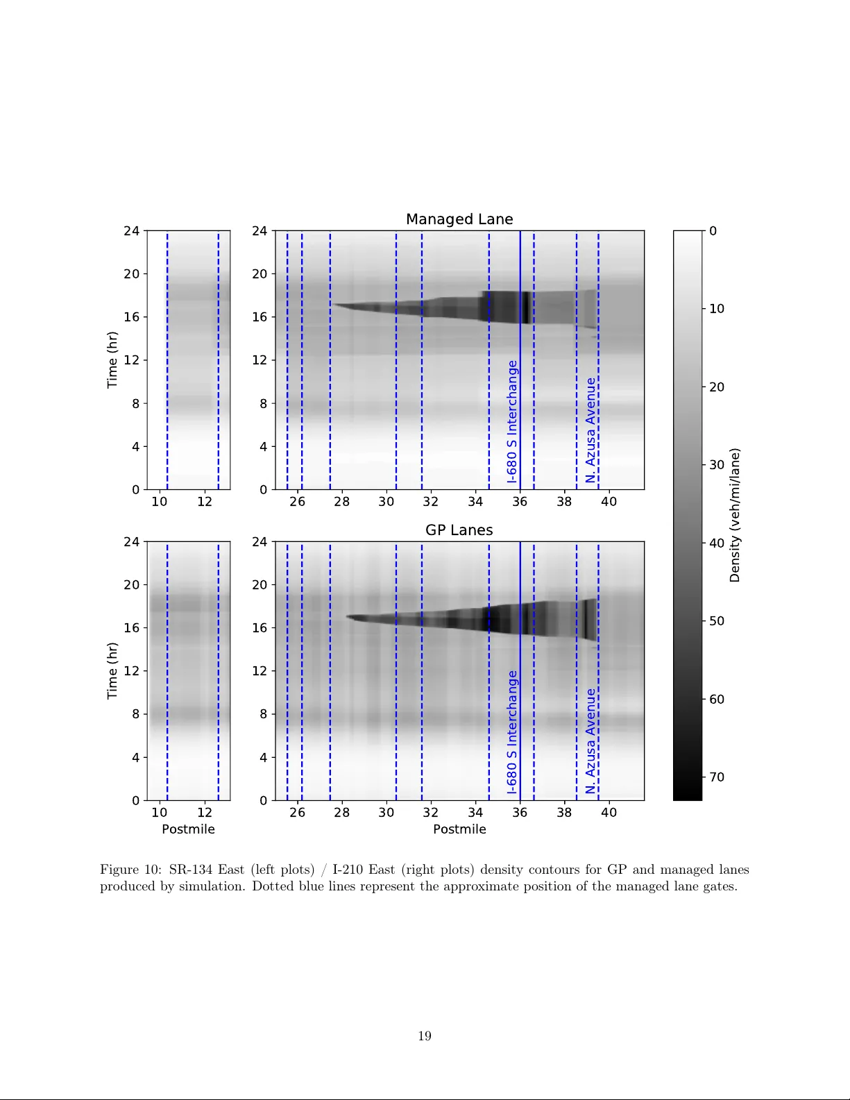
Macroscopic Mo deling, Calibration, and Sim ulation of Managed Lane-F reew a y Net w orks, P art I I: Net w ork-scale Calibration and Case Studies Matthew A. W righ t, Rob erto Horo witz, Alex A. Kurzhanskiy Abstract In P art I of this pap er series, several macroscopic traffic model elements for mathematically describing freew ay net works equipp ed with managed lane facilities were proposed. These mo deling tec hniques seek to capture at the macroscopic the complex phenomena that occur on managed lane-freewa y netw orks, where tw o parallel traffic flows interact with each other b oth in the physical sense (ho w and where cars flo w betw een the tw o lane groups) and the ph ysiological sense (how driving behaviors are changed by b eing adjacen t to a quantitativ ely and qualitatively differen t traffic flow). The lo cal descriptions we developed in P art I are not the only modeling complexity introduced in managed lane-freew a y net works. The complex top ologies mean that net work-scale mo deling of a freewa y corridor is increased in complexit y as well. The already-difficult mo del calibration problem for a dynamic mo del of a freewa y b ecomes more complex when the freewa y b ecomes, in effect, tw o interrelating flo w streams. In the presen t pap er, we presen t an iterative-learning-based approach to calibrating our mo del’s ph ysical and driver-behavioral parameters. W e consider the common situation where a complex traffic mo del needs to b e calibrated to recreate real-world baseline traffic b eha vior, such that counterfactuals can b e generated by training purp oses. Our metho d is used to identify traditional freew ay parameters as well as the prop osed parameters that describ e managed lane-freewa y-netw ork-sp ecific b eha viors. W e v alidate our model and calibration metho dology with case studies of simulations of tw o managed lane-equipp ed California freewa ys. Keyw ords : macroscopic first order traffic model, first order node mo del, m ulti-commo dit y traffic, man- aged lanes, HOV lanes, dynamic traffic assignment, dynamic netw ork loading, inertia effe ct, friction effect, smo othing effect 1 In tro duction Managed lanes (Ob enberger, No v/Dec 2004), such as high-o ccupancy-v ehicle (HOV) lanes or tolled lanes, ha ve b ecome a p opular p olicy tool for transportation authorities, who seek to capture b oth demand man- agemen t outcomes by incen tivizing b eha viors like carpo oling (Chang et al., 2008) and to gain additional real-time con trol ability (Kurzhanskiy and V araiya, 2015). In Part I of this pap er series (W right et al., 2019), we prop osed several macroscopic mo deling elemen ts for the purp ose of mathematically describing a freew ay equipp ed with a managed lane facility (a “managed lane-freew ay net work”). P art I discusses the road-top ological considerations of mo deling tw o parallel traffic flo ws, as well as mathematical descriptions for several of the complex emergen t (and sometimes counteracting) phenomena that hav e b een observed on managed lane-freew ay net works, like the so-called friction (Liu et al., 2011; Jang et al., 2012; Fitzpatrick et al., 2017) and smo othing (Menendez and Daganzo, 2007; Cassidy et al., 2010; Jang and Cassidy, 2012) effects. 1 The present pap er discusses the actual implemen tation of these mo deling constructions. T ransp ortation authorities considering a significant infrastructure in vestmen t lik e building new roads or installing managed lane facilities will mak e use of simulation to ols during the pre-construction planning phase (Caltrans Office of Pro ject Developmen t Pro cedures, 2011). Models let transp ortation planners understand the characteristics of the road net work, and predict outcomes of proposed mo difications b efore their undertaking. The use of models for the predictive study of coun terfactuals is esp ecially relev ant for managed lane de- plo yments. A ma jor b enefit of mo dern managed lanes to transp ortation authorities is how they can enable real-time, reactive control (Ob en b erger, Nov/Dec 2004; Kurzhanskiy and V araiya, 2015). Managed lanes to da y ma y be instrumented with operational capabilities for real-time traffic con trol, suc h as dynamic, condition-resp onsiv e toll rates in tolled express lanes (Lou et al., 2011). Real-time con trol decisions can b e studied via a w ell-tuned predictive mo del. As the traffic situation c hanges, m ultiple p oten tial op erational strategies can b e ev aluated to decide on the b est course of action. Before a traffic mo del can b e used for forecasting or generating counterfactuals, it must b e tuned to represent a base-case scenario, usually the existing traffic patterns. This pro cess of model tuning is generally referred to as c alibr ation . Calibration of traffic netw ork mo dels is kno wn to be a difficult task (T reib er and Kesting, 2013, Chapter 16): v ehicle traffic dynamics exhibit many complex and interacting nonlinear b ehaviors, and a mo del m ust realistically capture these behaviors to b e useful for analysis or planning purposes. F or a freew ay-corridor-scale net work, the data av ailable for model calibration ma y consist of v ehicle counts and mean speeds from v ehicle detectors, origin-destination surv ey data, and/or descriptive information about the regular spatiotemp oral exten t of regular. A calibration pro cess in volv es tuning a sim ulation mo del’s parameters suc h that it accurately repro duces typical traffic b eha viors (T reib er and Kesting, 2013). The nonlinear and chaotic nature of traffic means that calibrated parameter v alues t ypically cannot be found explicitly , and must be sought after via an iterativ e tuning-assessment pro cess. In this pap er, w e present a calibration metho dology for our recently-dev elop ed macroscopic managed lane- freew ay netw ork modeling constructions (W right et al., 2019), that in tegrates them into the broader macro- scopic traffic mo del calibration loop. Muc h of our fo cus is on iden tifying the split ratios, the p ortions of v ehicles that take each of several av ailable turns b et ween the managed lane(s) and the general-purp ose (GP) lane(s). These v alues are of particular imp ortance when the b ehavior of the managed lane is of in terest, and ha ve ma jor effects on the resulting analysis of managed lane usage and traffic b eha viors, but are not directly measurable with traditional traffic sensors. Instead, they must be found as part of the iterative calibration pro cess such that the macroscopic traffic patterns actually observ ed on the managed lane’s instrumentation are repro duced in the mo del. A managed lane-freewa y netw ork calibration pro cedure, in other w ords, is a sup erset of the calibration procedure for a typical freew ay corridor model. The remainder of this pap er is organized as follows. Section 2 outlines the macroscopic traffic model in question, whic h augmen ts the traditional kinematic-wa ve macroscopic traffic model with the managed-lane- sp ecific constructions developed in W righ t et al. (2019). Calibration pro cedures for the managed-lane-sp ecific comp onen ts, and the in tegration of them in to a full calibration lo op, is discussed in Section 3. T w o case studies of macroscopic mo deling of managed-lane-equipp ed freewa ys in California, one with a full-access managed lane and one with a separated managed lane with gated access, are presented in Section 4, follo wed b y concluding p oin ts in Section 5 2 A Managed Lane-F reew a y Net w ork Sim ulation Mo del In this Section, w e presen t a macroscopic sim ulation algorithm for managed lane-freewa y netw orks. This can be considered a fleshing-out of the simplified first-order macroscopic sim ulation metho d briefly outlined as context in W right et al. (2019), with extensions made by incorp orating the additional items w e described in the same pap er. 2 2.1 Bac kground “Macroscopic” traffic mo dels are those that mo del traffic flows via the con tinuum fluid approximation (orig- inally prop osed by Lighthill and Whitham (1955a,b); Richards (1956)) as opp osed to “microscopic” mo dels that mo del individual vehicles (T reiber and Kesting (2013) present a relatively recent broad survey of v ari- ous types of traffic mo dels). While macroscopic models necessarily hav e a low er resolution than microscopic mo dels, they make up for it in areas like shorter run times (making them useful for real-time operational analysis). The present pap er considers a macroscopic mo del for managed lane-freew ay netw orks, based on the family of “first-order,” “kinematic wa v e”-type mo dels descending from the Cell T ransmission Mo del (Daganzo, 1994, 1995). 2.2 Definitions • W e hav e a netw ork consisting of set of directed links L , representing segmen ts of road, and a set of no des N , whic h join the links. – A no de alwa ys has at least one incoming link and one outgoing link. – A link ma y hav e an upstream no de, a do wnstream no de, or both. • W e hav e C different v ehicle classes trav eling in the net work, with classes indexed b y c ∈ { 1 , . . . , C } . • Let t ∈ { 0 , . . . , T } denote the sim ulation timestep. • In addition, while we hav e not co v ered them here, the mo deler may optionally choose to define c ontr ol inputs to the sim ulated system that mo dify system parameters or the system state. Such control inputs may represent op erational traffic control sc hemes suc h as ramp metering, changeable message signs, a v ariable managed-lane p olicy , etc. In the con text of this pap er, w e suggest including the parameterization of the friction effect and the class-switc hing construction of the separated-access managed lane mo del to b e discussed in section 3.2 as control actions. 2.2.1 Link mo del definitions T raditionally , the mathematical equations that go vern the traffic flo w in the links are called the “link mo del.” • F or each link l ∈ L , let there b e a time-v arying C -dimensional state vector ~ ρ l ( t ) , which denotes the densit y of the link of each of the C vehicle classes at time t . – Eac h element of this vector, ρ c l ( t ) , up dates b etw een timestep t and timestep t + 1 according to (2.1). – Also define ρ c l, 0 for all l, c , the initial condition of the system. • W e define three types of links: – Ordinary links are those links that ha ve both b eginning and ending no des. – Origin links are those links that hav e only an ending no de. These links represent the roads that v ehicles use to enter the net work. – Destination links are those links that ha ve only a b eginning no de. These links represent the roads that v ehicles use to exit the netw ork. 3 • F or each link l ∈ L , define the actual parametric “link mo del” that computes the p er-class demands S c l ( t ) ≤ ρ c l ( t ) (the amount of vehicles that wan t to exit the link at time t ) and link supply R l ( t ) (the amoun t of v ehicles that link l can accept at time t ) as functions of t and ~ ρ l ( t ) . The particular link mo del equations is a mo deling choice, and man y authors hav e prop osed different versions. App endix A describ es a particular example link mo del that will b e used in the example sim ulations in Section 4. • F or eac h origin link l ∈ L , define a C -dimensional time-v arying vector, ~ d l ( t ) , where the c -th elemen t d c l ( t ) denotes the exogenous demand of class c in to the netw ork at link l . 2.2.2 No de mo del definitions Analogous to the link mo del, the equations that gov ern the traffic flows through no des (i.e., b et ween links) are called the “no de mo del.” • F or eac h node ν ∈ N , let i ∈ { 1 , . . . , M ν } denote the incoming links and j ∈ { 1 , . . . , N ν } denote the outgoing links. • F or each no de, define { β c ij ( t ) : P j β c ij ( t ) = 1 ∀ i, c } the time-v arying split ratios for each triplet { i, j, c } . Eac h split ratio may b e fully defined, partially defined, or fully undefined, with the undefined split ratios typically b eing the ones that sp ecify the crossflows b etw een the managed lane(s) and the GP lane(s). • F or each no de with both a managed lane link and a GP link exiting it, define a (state-dep enden t) split ratio solver for the managed lane-eligible v ehicles. W e suppose that the decision of eligible vehicles of whether or not to change b et ween the tw o lane t yp es is dep enden t on the lo cal traffic conditions. Appropriate metho ds for determining the desired lane type as a function of the current state may include logit-style discrete choice metho ds (F arhi et al., 2013) or dynamic-system-based mo dels such as the one prop osed in W righ t et al. (2018) and reviewed in App endix B. • F or eac h no de, define a “no de mo del” that, at eac h time t , takes its incoming links’ demands S c i ( t ) and split ratios β c ij ( t ) , its outgoing links’ supplies R j ( t ) , and other no dal parameters, and computes the flo ws f c ij ( t ) . As with the link mo del, the particular no de model equations is a mo deling c hoice, and m uch literature exists defining and analyzing different no de mo dels. In this pap er, we refer to a sp ecific no de mo del with a relaxed first-in-first-out (FIFO) construction that has additional parameters η i j 0 j ( t ) (m utual restriction interv als) and p i ( t ) (the incoming links’ priorities). Note also that a no de mo del with the relaxed FIFO construction can also b e used to pro duce the smo othing effect of managed lanes, as discussed in depth in P art I (W righ t et al., 2019). 2.2.3 State up date equation definitions These equations define the time ev olution of the states from time t to time t + 1 . • All links l ∈ L up date their states according to the equation ρ c l ( t + 1) = ρ c l ( t ) + 1 L l  f c l, in ( t ) − f c l, out ( t )  ∀ c ∈ { 1 , . . . , C } , (2.1) whic h is a slightly generalized form of a traditional m ulti-class CTM up date. • F or all ordinary and destination links, f c l, in ( t ) = M ν X i =1 f c il ( t ) , (2.2) where ν is the b eginning node of link l . 4 • F or all origin links, f c l, in ( t ) = d c l ( t ) . (2.3) • F or all ordinary and origin links, f c l, out ( t ) = N ν X j =1 f c lj ( t ) , (2.4) where ν is the ending no de of link l . • F or all destination links, f c l, out ( t ) = S c l ( t ) . (2.5) 2.3 Sim ulation algorithm 1. Initialization: ρ c l (0) := ρ c l, 0 t := 0 , for all l ∈ L , c ∈ { 1 , . . . , C } . 2. P erform all control inputs that hav e b een (optionally) sp ecified by the mo deler. F or our purp oses, this includes: (a) F or each managed lane link, mo dify the sending function of the link mo del in accordance with the friction effect mo del. As discussed in more detail in Part I (W righ t et al., 2019), for the particular link mo del of App endix A, our friction effect mo del is to mo dify the sending function of a managed lane link from (A.1) to S c ML ( t ) = ˆ v ML ( t ) ρ c ML ( t ) min ( 1 , ˆ F ML ( t ) ˆ v ML ( t ) P C c =1 ρ c ML ( t ) ) (2.6) where the subscript “ML” means that the symbols refer to the parameters of the managed lane link, and where the friction-adjusted free flo w sp eed ˆ V ML ( t ) and capacit y ˆ F ML ( t ) are ˆ v ML ( t ) = v f ML ( t ) − σ ML ∆ ML ( t ) (2.7) ˆ F ML ( t ) = ˆ v ML ( t ) ρ + ML (2.8) with n + ML the high critical density (see Appendix A for the definition), v f ML is the nominal free flo w sp eed for the managed lane link, σ ML ∈ [0 , 1] is the friction c o efficient of the managed lane link (which quantifies the degree to whic h the friction effect exerts its influence on the v ehicles in the link: Jang and Cassidy (2012) and others note that road configurations where the managed lane(s) and the GP lane(s) are more physically separated, e.g., a concrete barrier or traffic b ollards instead of only a painted line, hav e a lo wer magnitude of the friction effect), and ∆ ML ( t ) is the sp eed differential betw een the managed lane link and the GP link, ∆ 11 ( t ) = v f 11 − v 1 ( t − 1) . (2.9) (b) F or each managed lane link whose do wnstream no de is a gate no de in a gated-access managed lane configuration, perform class switching to ensure that vehicles realistically leav e the managed lane to tak e a downstream offramp, as detailed in W right et al. (2019). 5 3. F or each link l ∈ L and commo dity c ∈ { 1 , . . . , C } , compute the demand, S c l ( t ) using the link’s link mo del. 4. F or each ordinary and destination link l ∈ L , compute the supply R l ( t ) using the link mo del. F or origin links, the supply is not used. 5. F or each no de ν ∈ N that has one or more undefined split ratios β c ij ( t ) , use the no de’s split ratio solver to complete a fully-defined set of split ratios. Note that if an inertia effect mo del is b eing used, the mo dified split ratio solver, e.g. the one describ ed in Appendix B, should b e used where appropriate. 6. F or each node ν ∈ N , use the no de mo del to compute throughflows f c ij ( t ) for all i, j, c . 7. F or every link l ∈ L , compute the up dated state ~ ρ l ( t + 1) : • If l is an ordinary link, use (2.1), (2.2), and (2.4). • If l is an origin link, use (2.1), (2.3), and (2.4) • If l is a destination link, use (2.1), (2.2), and (2.5). 8. If t = T , then stop. Otherwise, incremen t t := t + 1 and return to step 2. 3 Calibrating the Managed Lane-F reew ay Net w ork Mo del T ypically , a traffic mo deler will ha ve some set of data collected from traffic detectors (e.g., velocity and flow readings), and will create a netw ork top ology with parameter v alues that allo w the mo del to repro duce these v alues in sim ulation. Then, the parameters can b e tw eaked to p erform prediction and analysis. F or our managed lane-freew ay net works, the parameters of interest are: 1. Link mo del parameters for eac h link (also called “fundamental diagram” parameters, referring to the graph drawn by the sending and receiving functions as functions of density). Calibration of a link mo del is t ypically agnostic to the node mo del and net work top ology , and there exists an abundan t literature on this topic. F or the pu rposes of the simulations in this work, we used the method of Dervisoglu et al. (2009), but an y other metho d is appropriate. 2. P ercentage of sp ecial (that is, able to access the managed lane) v ehicles in the traffic flow entering the system. This parameter dep ends on, e.g., the time of day and location as w ell as on the t yp e of managed lane. It could b e roughly estimated as a ratio of the managed lane v ehicle count to the total freew ay vehicle coun t during p eriods of congestion at any given location (supp osing of course that congestion in the GP lanes will lead the eligible vehicles to select the managed lane to av oid this congestion). 3. Inertia co efficien ts. These parameters affect only how traffic of different classes mixes in different links, but they ha ve no effect on the total v ehicle counts pro duced by the simulation. 4. F riction co efficien ts. Ho w to tune these parameters is an op en question. In Jang and Cassidy (2012) the dependency of a managed lane’s speed on the GP lane speed w as in vestigated under differen t densities of the managed lane, and the presented data suggests that although the correlation b et ween the tw o sp eeds exists, it is not ov erwhelmingly strong, below 0.4. Therefore, we suggest setting friction co efficien ts to v alues not exceeding 0 . 4 . 5. Mutual restriction interv als for the partial FIF O constraint. It is also an op en question how to estimate m utual restriction interv als from the measuremen t data. See the discussion in W right et al. (2019, Section 3.2) for some guidelines. Note also that the choice of restriction interv als gov ern the magnitude of the smo othing effect. 6 6. Offramp split ratios. Calibrating a traffic mo del, or iden tifying the b est v alues of its parameters to match real-w orld data, is t ypically an inv olved pro cess for all but the simplest netw ork topologies. In particular, once w e consider more than a single, unbrok en stretch of freewa y , the nonlinear nature and netw ork effects of these systems means that estimating eac h parameter in isolation might lead to unpredictable b eha vior. Instead, nonlinear and/or non-con vex optimization techniques such as genetic algorithms (Poole and K otsialos, 2012), particle sw arm metho ds (Poole and Kotsialos, 2016), and others (Ngo duy and Maher (2012); F ransson and Sandin (2012), etc.) are employ ed. In the managed lane-freewa y netw orks we ha ve discussed, the k ey unknown parameters w e hav e introduced are the offramp split ratios, item 6, which ma y b e particularly hard to estimate as they are typically time- v arying and explicitly represent driver b ehavior, rather than ph ysical parameters of the road. Estimating the v alues of the other parameters can be done with one of man y metho ds in the literature. The remainder of this section describ es iterativ e metho ds for iden tification of the offramp split ratios for b oth the full-access and gated-access top ological configurations, b oth of which were in tro duced in P art I (W right et al., 2019). 3.1 Split ratios for a full-access managed lane Figure 1: A no de where some of the input links form tra vel facilities with some of the output links. ML = Managed Lane. Consider a no de, one of whose output links is an offramp, as depicted in Figure 1. W e shall make the follo wing assumptions. 1. The total flow en tering the offramp, ˆ f in 222 , at any giv en time is known (from measurements) and is not restricted b y the offramp supply: ˆ f in 222 < R 222 . 2. The p ortions of traffic sent to the offramp from the managed lane and from the GP lane at an y given time are equal: β c 1 , 222 = β c 11 , 222 , β , c = 1 , . . . , C . 3. None of the flow coming from the onramp (link 111), if such flow exists, is directed tow ard the offramp. In other w ords, β c 111 , 222 = 0 , c = 1 , . . . , C . 4. The distribution of flow p ortions not directed to the offramp b et ween the managed lane and the GP output links is known. This can b e written as: β c ij = (1 − β ) δ c ij , where δ c ij ∈ [0 , 1] , as w ell as β 111 ,j , i = 1 , 11 , j = 2 , 22 , c = 1 , . . . , C , are kno wn. 5. The demand S c i , i = 1 , 11 , 111 , c = 1 , . . . , C , and supply R j , j = 2 , 22 , are giv en. A t any giv en time, β is unknown and is to b e found. 7 If β were kno wn, the no de mo del w ould compute the input-output flo ws, in particular, f i, 222 = P C c =1 f c i, 222 , i = 1 , 11 . Define ψ ( β ) = f 1 , 222 + f 11 , 222 − ˆ f in 222 . (3.1) Our goal is to find β from the equation ψ ( β ) = 0 , (3.2) suc h that β ∈ h ˆ f in 222 S 1 + S 11 , 1 i , where S i = P C c =1 S c i . Obviously , if S 1 + S 11 < ˆ f in 222 , the solution do es not exist, and the best we can do in this case to matc h ˆ f in 222 is to set β = 1 , directing all traffic from links 1 and 11 to the offramp. Supp ose now that S 1 + S 11 ≥ ˆ f in 222 . F or an y giv en ˆ f in 222 , w e assume ψ ( β ) is a monotonically increasing function of β (this assumption is true for the particular node mo del of W righ t et al. (2017)). Moreo ver, ψ  ˆ f in 222 S 1 + S 11  ≤ 0 , while ψ (1) ≥ 0 . Thus, the solution of (3.2) within the giv en in terv al exists and can be obtained using the bise ction metho d . The algorithm for finding β follo ws. 1. Initialize: b (0) := ˆ f in 222 S 1 + S 11 ; b (0) := 1; k := 0 . 2. If S 1 + S 11 ≤ ˆ f in 222 , then are not enough v ehicles to satisfy the offramp demand. Set β = 1 and stop. 3. Use the no de mo del with β = b (0) and ev aluate ψ ( β ) . If ψ ( b (0)) ≥ 0 , then set β = b (0) and stop. 4. Use the no de model with β = b ( k )+ b ( k ) 2 and ev aluate ψ ( β ) . If ψ  b ( k )+ b ( k ) 2  = 0 , then set β = b ( k )+ b ( k ) 2 and stop. 5. If ψ  b ( k )+ b ( k ) 2  < 0 , then up date: b ( k + 1) = b ( k ) + b ( k ) 2 ; b ( k + 1) = b ( k ) . Else, up date: b ( k + 1) = b ( k ); b ( k + 1) = b ( k ) + b ( k ) 2 . 6. Set k := k + 1 and return to step 4. Here, b ( k ) represen ts the low er b ound of the search interv al at iteration k and b ( k ) the upper b ound. 8 3.2 Split ratios for the separated managed lane with gated access The configuration of a no de with an offramp as one of the output links is simpler in the case of a separated managed lane, as shown in Figure 2. Here, traffic cannot directly go from the managed lane to link 222, and, thus, w e ha ve to deal only with the 2-input-2-output no de. There is a cav eat, how ever. Recall from the discussion of gated-access managed lanes in W righ t et al. (2019) that in the separated managed lane case w e hav e destination-based traffic classes, and split ratios for destination-based traffic are fixed due to b eing determined at an outer lo op level. Figure 2: A no de with a GP link and an onramp as inputs, and a GP link and an offramp as outputs. W e shall make the follo wing assumptions: 1. The total flow en tering the offramp, ˆ f in 222 , at any giv en time is known (from measurements) and is not restricted b y the offramp supply: ˆ f in 222 < R 222 . 2. All the flo w coming from the onramp (link 111), if such flo w exists, is directed tow ard the G P link 2. In other w ords, β c 111 , 2 = 1 and β c 111 , 222 = 0 , c = 1 , . . . , C . 3. The demand S c i , i = 1 , 111 , c = 1 , . . . , C , and supply R 2 are giv en. 4. W e denote the set of destination-based classes as D . The split ratios β c 1 j for c ∈ D are kno wn. Let the split ratios β c 1 j = β for c ∈ { 1 , . . . , C } \ D , where β is to b e determined (i.e., w e assume all non-destination-based classes exit at the same rate). The first three assumptions here repro duce assumptions 1, 3 and 5 made for the full-access managed lane case. Assumption 4 is a reminder that there is a p ortion of traffic flow that we cannot direct to or aw ay from the offramp, but w e hav e to account for it. Similarly to the full-access managed lane case, w e define the function ψ ( β ) : ψ ( β ) = X c ∈D f c 1 , 222 + X c ∈D f c 1 , 222 − ˆ f in 222 , (3.3) where f c 1 , 222 , c = 1 , . . . , C are determined by the no de model. The first term of the right-hand side of (3.3) dep ends on β . As b efore, w e assume ψ ( β ) is a monotonically increasing function. W e lo ok for the solution of equation (3.2) on the interv al [0 , 1] . This solution exists iff ψ (0) ≤ 0 and ψ (1) ≥ 0 . The algorithm for finding β is the same as the one presented in the previous section, except that b (0) should b e initialized to 0 , and S 11 is to b e assumed 0 . 3.3 An iterative full calibration pro cess F or the purp oses of the sim ulations presen ted in the follo wing Section, we placed the iterative split ratio iden tification metho ds of Sections 3.1 and 3.2 within a larger iterative lo op for the remaining parameters. The mo del calibration follows the flo wc hart shown in Figure 3. 9 Figure 3: Calibration workflo w. 1. W e start by assembling the a v ailable measuremen t data. F undamen tal diagrams are assumed to b e giv en. Mainline and onramp demand are sp ecified p er 5-minute p eriods together with the sp ecial vehicle p ortion parameter indicating the fraction of the input demand that is able to access the managed lane. Initially , we do not know offramp split ratios as they cannot b e measured directly . Instead, we use some arbitrary v alues to represent them and call these v alues “initially guessed offramp split ratios”. Instead of the offramp split ratios, w e ha ve the measured flows actually observed on the offramps, which we refer to as offr amp demand . 2. W e run our net work simulation outlined in Section 2.3 for the entire simulation p erio d. A t this p oin t, in step 5 of the sim ulation, the a priori undefined split ratios b et w een traffic in the GP and in the managed lanes are assigned using a split ratio solver. 3. Using these newly-assigned split ratios, we run our netw ork simulation again, only this time, instead of using the initially guessed offramp split ratios, we compute them from the given offramp demand as describ ed in Sections 3.1 and 3.2. As a result of this step, w e obtain new offramp split ratios. 4. No w we run the net work simulation as w e did originally , in step 2, only this time with new offramp split ratios, and record the sim ulation results — densit y , flow, sp eed, as w ell as performance measures suc h as vehicle miles tra veled (VMT) and vehicle hours tra veled (VHT). 5. Chec k if the resulting offramp flows matc h the offramp demand. If yes, pro ceed to step 6, otherwise, rep eat steps 2-5. In our exp erience (i.e., the case studies in the follo wing Section), it takes the process describ ed in steps 2-5 no more than tw o iterations to conv erge. 6. Ev aluate the simulation results: • correctness of b ottlenec k lo cations and activ ation times; • correctness of congestion extension at eac h b ottlenec k; • correctness of VMT and VHT. If the sim ulation results are satisfactory , stop. Otherwise, pro ceed to step 7. 7. T une/correct input data in the order shown in block 7 of Figure 3. 4 Sim u lation Results 4.1 F ull-access managed lane case study: In terstate 680 North W e consider a 26.8-mile stretch of I-680 North freewa y in Contra Costa Count y , California, from p ostmile 30 to p ostmile 56.8, sho wn in Figure 4, as a test case for the full-access managed lane configuration. This 10 freew ay’s managed lane facilities are split into t wo segmen ts whose b eginning and end p oin ts are mark ed on the map. The first segment is a high-o ccupancy-tolled (HOT) lane, which allows free entry to vehicles with tw o or more passengers and tolled entry to single-o ccupancy vehicles (Metropolitan T ransp ortation Commission, 2019), The second segment has an HOV lane is 4.5 miles long. There are 26 onramps and 24 offramps. The HO V lane is active from 5 to 9 AM and from 3 to 7 PM. The rest of the time, the HO V lane is op en to all traffic, and b ehav es as a GP lane. Figure 4: Map of I-680 North in Contra Costa Coun ty . T o build the mo del, we used data collected for the I-680 Corridor System Managemen t Plan (CSMP) study (System Metrics Group, Inc., 2015). The b ottlenec k lo cations as well as their activ ation times and congestion extension were identified in that study using video monitoring and tachometer vehicle runs. On- and offramp flo ws were given in 5-min ute increments. F or the purp oses of our mo del, we do not consider tolling dynamics, and instead assume that managed lane-eligible vehicles incur no cost to access the man- aged lane. W e assume that the managed lane-eligible p ortion of the input demand is 15%. The mo del was calibrated to a t ypical weekda y , as suggested in the I-680 CSMP study . F or this sim ulation, we used the fundamen tal diagram described in Appendix A, with parameters as follows: • The capacit y of the ordinary GP lane is 1,900 vehicles per hour p er lane (vphl); • The capacit y of the auxiliary GP lane is 1,900 vphl; • The capacity of the managed lane is 1,800 vphl while activ e and 1,900 vphl when it b eha ves as a GP lane; • The free flow sp eed v aries b et ween 63 and 70 mph — these measuremen ts came partially from the California P erformance Measuremen t System (PeMS) (PeMS, 2019) and partially from tachometer v ehicle runs. • The congestion w av e sp eed for eac h link was taken as 1 / 5 of the free flo w sp eed. The mo deling results are presented in Figures 5, 6 and 7 showing density , flow and sp eed contours, resp ec- tiv ely , in the GP and the managed lanes. In each plot, the top contour corresp onds to the managed lanes, 11 and the b ottom to the GP lanes. In all the plots traffic mov es from left to right along the “Absolute Postmile” axis, while the v ertical axis represents time. Bottleneck lo cations and congestion areas identified by the I-680 CSMP study are mark ed b y blue b o xes in GP lane con tours. The managed lane does not get congested, but there is a sp eed drop due to the friction effect. The friction effect, when vehicles in the managed lane slow do wn b ecause of the slo w mo ving GP lane traffic, can b e seen in the managed lane sp eed contour in Figure 7. Figure 8 sho ws an example of how w ell the offramp flow computed by the simulation matc hes the target, referred to as offr amp demand , as recorded by the detector on the offramp at Crow Cany on Road. W e can see that in the beginning and in the end of the day , the computed flow falls below the target (corresp onding areas are marked with red circles). This is due to the shortage of the mainline traffic in the sim ulation — the offramp demand cannot b e satisfied. Finally , T able 1 summarizes the p erformance metrics — vehicle miles trav eled (VMT), v ehicle hours trav eled (VHT) and delay in vehicle-hours — computed b y simulation versus those collected in the course of the I-680 CSMP study . Dela y is computed for vehicles with sp eed b elo w 45 mph. P erformance Metric Sim ulation result Collected data GP Lane VMT 1,687,618 - Managed Lane VMT 206,532 - T otal VMT 1,894,150 1,888,885 GP Lane VHT 27,732 - Managed Lane VHT 3,051 - T otal VHT 30,783 31,008 GP Lane Dela y (hr) 2,785 - Managed Lane Dela y (hr) 6 - T otal Delay (hr) 2,791 2,904 T able 1: P erformance metrics for I-680 North. 12 Figure 5: I-680 North density contours for GP and managed lanes pro duced b y simulation. Densit y v alues are given in vehicles p er mile p er lane. Blue b o xes on the GP lane speed con tour indicate congested areas as iden tified by the I-680 CSMP study . 13 Figure 6: I-680 North flow contours for GP and managed lanes pro duced b y sim ulation. Flow v alues are giv en in vehicles p er hour p er lane. Blue b o xes on the GP lane sp eed contour indicate congested areas as iden tified by the I-680 CSMP study . 14 Figure 7: I-680 North sp eed con tours for GP and managed lanes pro duced b y simulation. Speed v alues are giv en in miles p er hour. Blue b o xes on the GP lane sp eed con tour indicate congested areas as identified b y the I-680 CSMP study . 15 Figure 8: Flo w at the Crow Cany on Road offramp ov er 24 hours — collected (offramp demand) vs. computed b y simulation (offramp flo w). 16 4.2 Gated-access managed lane case study: Interstate 210 East W e consider a 20.6-mile stretc h of SR-134 East/ I-210 East in Los Angeles Count y , California, shown in Figure 9, as a test case for the separated managed lane configuration. This freewa y’s managed lane is also an HOV lane. This freewa y stretc h consists of 3.9 miles of SR-134 East from p ostmile 9.46 to p ostmile 13.36, whic h merges into 16.7 miles of I-210 East from p ostmile 25 to p ostmile 41.7. Gate lo cations where traffic can switc h b et ween the GP and the HOV lanes are marked on the map. At this site, the HOV lane is alwa ys activ e. There are 28 onramps and 25 offramps. The largest num b er of offramps b et ween tw o gates is 5. Th us, our freewa y model has 7 v ehicle classes - LO V (low-occupancy v ehicles; not managed lane-eligible), HO V (managed lane-eligible) and 5 destination-based. Figure 9: Map of SR-134 East/ I-210 East freewa y in Los Angeles Count y . T o build the mo del, w e used PeMS data for the corresp onding segments of the SR-134 East and I-210 East for Monda y , Octob er 13, 2014 (PeMS, 2019). F undamental diagrams were calibrated using PeMS data following the metho dology of Dervisoglu et al. (2009). As in the I-680 North example, w e assume that the managed lane-eligible p ortion of the input demand is 15%. The modeling results are presen ted in Figures 10, 11 and 12 showing density , flo w and sp eed con tours, resp ectiv ely , in the GP and the managed lanes. In each plot, the top contour corresp onds to the managed lanes, and the b ottom to the GP lanes. As b efore, in all the plots traffic mov es from left to right along the “Absolute Postmile” axis, while the vertical axis represen ts time. The managed lane does not get congested. Dashed blue lines on the con tour plots indicate managed gate lo cations. Figure 13 sho ws the PeMS sp eed contours for the SR-134 East/ I-210 East GP and managed lanes that were used as a target for our simulation mo del. In these plots, traffic also trav els from left to righ t, with the horizon tal axis representing postmiles, while the vertical axis represen ts time. Figure 14 shows an example of how well the offramp flow computed b y the simulation matches the target, referred to as offr amp demand , as recorded b y the detector on the offramp at North Hill A ven ue. The sim ulated offramp flow matc hes the offramp demand fairly closely . Similar results were found for the other offramps. Finally , T able 2 summarizes the p erformance metrics — VMT, VHT and delay — computed by sim ulation v ersus those v alues obtained from PeMS. The P eMS data come from b oth SR-134 East and I-210 East, and VMT, VHT and dela y v alues are computed as sums of the corresp onding v alues from these tw o freewa y sections. Delay v alues are computed in vehicle-hours for those vehicles tra veling slow er than 45 mph. 17 P erformance metric Sim ulation result P eMS data GP Lane VMT 2,017,322 - Managed Lane VMT 378,485 - T otal VMT 2,395,807 414,941 + 2,006,457 = 2,421,398 GP Lane VHT 33,533 - Managed Lane VHT 6,064 - T otal VHT 39,597 6,416 + 36,773 = 43,189 GP Lane Dela y (hr) 3,078 - Managed Lane Dela y (hr) 584 - T otal Delay (hr) 3,662 1 + 3,802 = 3,803 T able 2: P erformance metrics for SR-134 East/ I-210 East. 18 10 12 0 4 8 12 16 20 24 Time (hr) 26 28 30 32 34 36 38 40 0 4 8 12 16 20 24 I-680 S Interchange N. Azusa Avenue Managed Lane 10 12 Postmile 0 4 8 12 16 20 24 Time (hr) 26 28 30 32 34 36 38 40 Postmile 0 4 8 12 16 20 24 I-680 S Interchange N. Azusa Avenue GP Lanes 0 10 20 30 40 50 60 70 Density (veh/mi/lane) Figure 10: SR-134 East (left plots) / I-210 East (right plots) density contours for GP and managed lanes pro duced by sim ulation. Dotted blue lines represen t the approximate p osition of the managed lane gates. 19 10 12 0 4 8 12 16 20 24 Time (hr) 26 28 30 32 34 36 38 40 0 4 8 12 16 20 24 I-680 S Interchange N. Azusa Avenue Managed Lane 10 12 Postmile 0 4 8 12 16 20 24 Time (hr) 26 28 30 32 34 36 38 40 Postmile 0 4 8 12 16 20 24 I-680 S Interchange N. Azusa Avenue GP Lanes 0 250 500 750 1000 1250 1500 1750 2000 Flow (veh/hr/lane) Figure 11: SR-134 East (left plots) / I-210 East (righ t plots) flo w contours for GP and managed lanes pro duced by sim ulation. Dotted blue lines represen t the approximate p osition of the managed lane gates. 20 10 12 0 4 8 12 16 20 24 Time (hr) 26 28 30 32 34 36 38 40 0 4 8 12 16 20 24 I-680 S Interchange N. Azusa Avenue Managed Lane 10 12 Postmile 0 4 8 12 16 20 24 Time (hr) 26 28 30 32 34 36 38 40 Postmile 0 4 8 12 16 20 24 I-680 S Interchange N. Azusa Avenue GP Lanes 0 10 20 30 40 50 60 70 Speed (mi/hr) Figure 12: SR-134 East (left plots) / I-210 East (righ t plots) sp eed contours for GP and managed lanes pro duced by sim ulation. Dotted blue lines represen t the approximate p osition of the managed lane gates. 21 Figure 13: SR-134 East/ I-210 East sp eed con tours for GP and managed lanes obtained from P eMS for Monda y , Octob er 13, 2014. The horizontal axis represents absolute p ostmile, and the vertical axis represents time in hours. Note the four contours share the same color scale. 22 Figure 14: Flow at the North Hill A v enue offramp o ver 24 hours — P eMS data (offramp demand) vs. computed b y simulation (offramp flo w). 23 4.3 Discussion As we men tion in section 3, a common calibration goal for traffic mo delers is to create a simulation that can accurately recreate a “base case” of a t ypical real-world day’s traffic patterns; this calibrated “base case” can then b e t weak ed to predict the system-wide effects of coun terfactual ev ents suc h as a global demand increase, a lo calized lane closure, etc. One traditional criterion for ev aluating whether a freew ay mo del captures this “base case” is whether the sim ulation predicts congestion at the same time and the same place as in real-world data (and, if the dynamic b eha viors such as the rate of the buildup of the queue and the rate of queue discharge are similar). In this congestion-lo calit y criterion, our sim ulation case studies p erform well. F or the case study of I-680 North, examining Figures 5 through 7 w e see that our models predict congestion originating at the b ottlenec k lo cations and propagating to the exten ts iden tified in the CSMP study (System Metrics Group, Inc., 2015). F or the SR-134 East / I-210 East, we can compare the reference P eMS lo op data sp eed con tour (Figure 13) to our sim ulations (Figures 10-12). The PeMS data show and out sim ulations predict congestion in b oth the managed lane and the GP lanes that originates at a b ottlenec k at N. Azusa A ven ue at roughly 15:00, propagates backw ard in space until reaching its maxim um spatial extent roughly at p ostmile 29 at ab out 17:00, and then recedes until fully dissipating at roughly 19:00. The managed lane data from the P eMS dataset (Figure 13) has more iden tifiable w av efronts propagating backw ard and receding forw ard than the GP lanes, and those w av efront’s sp eeds agree somewhat with those predicted by the simulation (unfortunately , a definitiv e v alue for the true w av efront sp eed is difficult to obtain due to the low resolution of the P eMS data). Bey ond the somewhat qualitativ e examination of whether the macroscopic congestion matters match reality , w e can also ev aluate quantitativ ely whether our simulation fits the a v ailable measuremen ts from the site. Figures 8 and 14 sho w how our model matc hed the offramp flo w at the t wo identified b ottlenecks of the case study sites. Both figures show agreement b et w een mo del and data. Note that this “offramp demand” w as an explicit calibration target (as describ ed in section 3.3). So, close matc hing of this is an explici t requisite for the calibrated mo del, and, it is necessary that the offramp flow here be satisfied, and the flow that does not take the offramp still pro duce the congestion patterns as discussed in the previous paragraph. These t wo offramp flow figures can b e interpreted as stating Neumann (flux) b oundary conditions that our freewa y PDE mo del must (and does) fulfill, in addition to the macro-scale congestion requiremen ts. Finally , T ables 1 and 2 show macroscopic freewa y p erformance metrics predicted b y our sim ulation and the comparable measured p erformance metrics. F or the three quantities for whic h measured p erformance metrics are a v ailable (total VMT, total VHT, and total delay), we can see that all percentage errors b etw een our sim ulation and the measurements are at most roughly 10%. W e consider this is a fairly go od accuracy , given the inherent high noise of p erformance metrics computed from stationary sensors lik e the lo op detectors used b y P eMS (Jia et al., 2001; Chen et al., 2003). In particular, we find higher errors betw een the sim ulated p erformance metrics and the measured p erformance metrics for the SR-134 East / I-210 East case study , a lo cation where single-lo op detectors are presen t, than for the I-680 North case study , where mostly dual-lo op detectors are presen t (P eMS, 2019) (single-lo op detectors b eing intrinsically muc h more noisy than dual-lo op detectors at measuring quan tities like speed and flow (Jia et al., 2001)). 5 Conclusion This pap er presented the implemen tation of the mo deling comp onen ts for managed lane-freew ay netw orks originally prop osed in W right et al. (2019). This included their integration in to b oth a full macroscopic traffic mo del suitable for corridor-scale traffic sim ulation and analysis, as well as fitting in estimation methods for some of the harder-to-estimate parameters into the traditional iterative calibration approach for traffic mo dels. 24 Our simulation results comparing our mo del and calibration results sho wed goo d agreement in t wo case studies, v alidating b oth our full-access and gated-access mo deling tec hniques. In the sequel to this pap er series, w e will further extend these results to include simulation and study of traffic con trol, with a reactiv e tolling con troller on the managed lane. A c kno wledgemen ts W e w ould lik e to express great appreciation to sev eral of our colleagues. T o Elena Dorogush and Ajith Muralidharan for sharing ideas, and to Gabriel Gomes and Pravin V araiya for their critical reading and their help in clarifying some theoretical issues. This researc h was supp orted b y the California Department of T ransp ortation. Earlier versions of some of this article’s material previously app eared in the technical report Horo witz et al. (2016). A A link Mo del Figure 15: The “backw ards lambda” fundamen tal diagram. F or the ma jorit y of this work, we remain agnostic as to the particular functional relationship b et ween density ρ l , demand S l (p er commo dit y , ρ c l , S c l ) and supply R l , and flo w f l (also called the fundamental diagram) used in our first-order macroscopic mo del. F or the simulation results presented in section 4, we use a particular link mo del sho wn in Figure 15. This fundamental diagram captures the traffic hysteresis b eha vior with the “bac kwards lam b da” shap e often observ ed in detector data (Koshi et al., 1983): S c l ( t ) = v f l ( t ) ρ c l ( t ) min ( 1 , F l ( t ) v f l ( t ) P C c =1 ρ c l ( t ) ) , S l ( t ) = C X c =1 S c l ( t ) , (A.1) R l ( t ) = (1 − θ l ( t )) F l ( t ) + θ l ( t ) w l ( t ) ρ J l ( t ) − C X c =1 ρ c l ( t ) ! , (A.2) where, for li nk l , F l is the capacity , v f l is the free flo w speed, w l is the congestion w av e sp eed, ρ J l is the jam density , and ρ − l = w l ρ J l v f l + w l and ρ + l = F l v f l are called the low and high critic al densities , resp ectiv ely . As written here and used in this work, F l , v f l , and w l are in units p er simulation timestep. The v ariable θ l ( t ) is a congestion metastate of l , which encodes the hysteresis: θ l ( t ) =      0 ρ l ( t ) ≤ ρ − l , 1 ρ l ( t ) > ρ + l , θ l ( t − 1) ρ − l < ρ l ( t ) ≤ ρ + l , (A.3) 25 where ρ l ( t ) = P C c =1 ρ c l ( t ) . Examining (A.3) and (A.2), we see that when a link’s density go es ab o ve ρ + l (i.e., when it b ecomes congested), its abilit y to receive flo w is reduced until the density falls below ρ − l . An image of (A.1) and (A.2) ov erlaid on eac h other, giving a schematic image of the fundamental diagram, is shown in Figure 15. Unless ρ − l = ρ + l , when it assumes triangular shap e, the fundamental diagram is not a function of densit y alone (i.e., without θ l ( t ) ): ρ l ( t ) ∈  ρ − l , ρ + l  admits t wo possible flow v alues. B Dynamic Split Ratio Solv er Throughout this article, we ha ve made reference to a dynamic-system-based metho d for solving for partially- or fully-undefined split ratios from W right et al. (2017). This split ratio solver is designed to implicitly solve the logit-based split ratio problem β c ij = exp  P M i =1 P C c =1 S c ij R j  P N j 0 =1 exp  P M i =1 P C c =1 S c ij 0 R j 0  , (B.1) whic h cannot b e solv ed explicitly , as the S c ij ’s are also functions of the β c ij ’s. The problem (B.1) is chosen to b e a no de-lo cal problem that does not rely on information from the link mo del (b ey ond supplies and demands), and is th us indep enden t of the choice of link model (W right et al., 2017). The solution algorithm is as follo ws, repro duced from W right et al. (2017). More discussion is av ailable in the reference. • Define the set of commo dit y mov ements for which split ratios are known as B =  { i, j, c } : β c ij ∈ [0 , 1]  , and the set of commo dity mov ements for which split ratios are to b e computed as B =  { i, j, c } : β c ij are unkno wn  . • F or a given input link i and commo dity c such that S c i = 0 , assume that all split ratios are kno wn: { i, j, c } ∈ B . 1 • Define the set of output links for whic h there exist unknown split ratios as V =  j : ∃ { i, j, c } ∈ B  . • Assuming that for a given input link i and commodity c , the split ratios m ust sum up to 1, define the unassigned p ortion of flow b y β c i = 1 − P j : { i,j,c }∈B β c ij . • F or a given input link i and commo dity c suc h that there exists at least one commo dit y mo vemen t { i, j, c } ∈ B , assume β c i > 0 , otherwise the undefined split ratios can b e trivially set to 0. • F or ev ery output link j ∈ V , define the set of input links that ha ve an unassigned demand p ortion directed to ward this output link b y U j =  i : ∃ { i, j, c } ∈ B  . • F or a giv en input link i and commo dity c , define the set of output links for whic h split ratios for whic h are to b e computed as V c i = { j : ∃ i ∈ U j } , and assume that if nonempty , this set con tains at least t wo elemen ts, otherwise a single split ratio can b e trivially set equal to β c i . • Assume that input link priorities are non-negativ e, p i ≥ 0 , i = 1 , . . . , M , and P M i =1 p i = 1 . 1 If split ratios were undefined in this case, they could b e assigned arbitrarily . 26 • Define the set of input links with zero priorit y: U z p = { i : p i = 0 } . T o enable split ratio assignment for inputs with zero priorities, p erform regularization: ˜ p i = p i  1 − | U z p | M  + 1 M | U z p | M = p i M − | U z p | M + | U z p | M 2 , (B.2) where | U z p | denotes the num b er of elements in set U z p . Expression (B.2) implies that the regularized input priority ˜ p i consists of tw o parts: (1) the original input priorit y p i normalized to the p ortion of input links with positive priorities; and (2) uniform distribution among M input links, 1 M , normalized to the p ortion of input links with zero priorities. Note that the regularized priorities ˜ p i > 0 , i = 1 , . . . , M , and P M i =1 ˜ p i = 1 . The algorithm for distributing β c i among the commo dit y mov ements in B (that is, assigning v alues to the a priori unknown split ratios) aims at maintaining output links as uniform in their demand-supply ratios as p ossible. At each iteration k , t wo quantities are identified: µ + ( k ) , which is the largest oriente d demand- supply ratio pro duced by the split ratios that ha ve b een assigned so far, and µ − ( k ) , which is the smallest orien ted demand-supply ratio whose input link, denoted i − , still has some unclaimed split ratio. Once these t wo quantities are found, the commo dit y c − in i − with the smallest unallocated demand has some of its demand directed to the j corresp onding to µ − ( k ) to bring µ − ( k ) up to µ + ( k ) (or, if this is not p ossible due to insufficien t demand, all such demand is directed). T o summarize, in eac h iteration k , the algorithm attempts to bring the smallest oriented demand-supply ratio µ + ( k ) up to the largest oriented demand-supply ratio µ − ( k ) . If it turns out that all such oriented demand-supply ratios b ecome p erfectly balanced, then the demand-supply ratios ( P i P c S c ij ) /R j are as w ell. The algorithm is: 1. Initialize: ˜ β c ij (0) :=  β c ij , if { i, j, c } ∈ B , 0 , otherwise ; β c i (0) := β c i ; ˜ U j (0) = U j ; ˜ V (0) = V ; k := 0 , Here ˜ U j ( k ) is the remaining set of input links with some unassigned demand, which may b e directed to output link j ; and ˜ V ( k ) is the remaining set of output links, to which the still-unassigned demand ma y b e directed. 2. If ˜ V ( k ) = ∅ , stop. The sought-for split ratios are n ˜ β c ij ( k ) o , i = 1 , . . . , M , j = 1 , . . . , N , c = 1 , . . . , C . 3. Calculate the remaining unallo cated demand: S c i ( k ) = β c i ( k ) S c i , i = 1 , . . . , M , c = 1 , . . . , C. 4. F or all input-output link pairs, calculate oriented demand: ˜ S c ij ( k ) = ˜ β c ij ( k ) S c i . 27 5. F or all input-output link pairs, calculate oriented priorities: ˜ p ij ( k ) = ˜ p i P C c =1 γ c ij S c i P C c =1 S c i (B.3) with γ c ij ( k ) = ( β c ij , if split ratio is defined a priori: { i, j, c } ∈ B , ˜ β c ij ( k ) + β c i ( k ) | V c i | , otherwise , (B.4) where | V c i | denotes the num b er of elements in the set V c i . Examining the expression (B.3)-(B.4), one can see that the split ratios ˜ β c ij ( k ) , whic h are not fully defined yet, are complemented with a fraction of β c i ( k ) inv ersely prop ortional to the n umber of output links among which the flow of commo dit y c from input link i can b e distributed. Note that in this step we are using r e gularize d priorities ˜ p i as opp osed to the original p i , i = 1 , . . . , M . This is done to ensure that inputs with p i = 0 are not ignored in the split ratio assignmen t. 6. Find the largest orien ted demand-supply ratio: µ + ( k ) = max j max i P C c =1 ˜ S c ij ( k ) ˜ p ij ( k ) R j X i ∈ U j ˜ p ij ( k ) . 7. Define the set of all output links in ˜ V ( k ) , where the minimum of the oriented demand-supply ratio is ac hieved: Y ( k ) = arg min j ∈ ˜ V ( k ) min i ∈ ˜ U j ( k ) P C c =1 ˜ S c ij ( k ) ˜ p ij ( k ) R j X i ∈ U j ˜ p ij ( k ) , and from this set pick the output link j − with the smallest output demand-supply ratio (when there are m ultiple minimizing output links, any of the minimizing output links ma y b e c hosen as j − ): j − = arg min j ∈ Y ( k ) P M i =1 P C c =1 ˜ S c ij ( k ) R j . 8. Define the set of all input links, where the minimum of the oriented demand-supply ratio for the output link j − is ac hieved: W j − ( k ) = arg min i ∈ ˜ U j − ( k ) P C c =1 ˜ S c ij − ( k ) ˜ p ij − ( k ) R j − X i ∈ U j − ˜ p ij − ( k ) , and from this set pick the input link i − and commo dit y c − with the smallest remaining unallo cated demand: { i − , c − } = arg min i ∈ W j − ( k ) , c : β c i − ( k ) > 0 S c i ( k ) . 9. Define the smallest orien ted demand-supply ratio: µ − ( k ) = P C c =1 ˜ S c i − j − ( k ) ˜ p i − j − ( k ) R j − X i ∈ U j − ˜ p ij − ( k ) . 28 • If µ − ( k ) = µ + ( k ) , the oriented demands created by the split ratios that hav e b een assigned as of iteration k , ˜ β c ij ( k ) , are p erfectly balanced among the output links, and to maintain this, all remaining unassigned split ratios should b e distributed prop ortionally to the allo cated supply: ˜ β c ij ( k + 1) = ˜ β c ij ( k ) + R j P j 0 ∈ V c i ( k ) R j 0 β c i ( k ) , c : β c i ( k ) > 0 , i ∈ ˜ U j ( k ) , j ∈ ˜ V ( k ); (B.5) β c i ( k + 1) = 0 , c : β c i ( k ) > 0 , i ∈ ˜ U j ( k ) , j ∈ ˜ V ( k ); ˜ U j ( k + 1) = ∅ , j ∈ ˜ V ( k ); ˜ V ( k + 1) = ∅ . If the algorithm ends up at this p oin t, we hav e emptied ˜ V ( k + 1) and are done. • Else, assign: ∆ ˜ β c − i − j − ( k ) = min    β c − i − ( k ) ,   µ + ( k ) ˜ p i − j − ( k ) R j − S c − i − ( k ) P i ∈ U j − ˜ p ij − ( k ) − P C c =1 ˜ S c i − j − ( k ) S c − i − ( k )      ; (B.6) ˜ β c − i − j − ( k + 1) = ˜ β c − i − j − ( k ) + ∆ ˜ β c − i − j − ( k ); (B.7) β c − i − ( k + 1) = β c − i − ( k ) − ∆ ˜ β c − i − j − ( k ); (B.8) ˜ β c ij ( k + 1) = ˜ β c ij ( k ) for { i, j, c } 6 = { i − , j − , c − } ; β c i ( k + 1) = β c i ( k ) for { i, c } 6 = { i − , c − } ; ˜ U j ( k + 1) = ˜ U j ( k ) \ n i : β c i ( k + 1) = 0 , c = 1 , . . . , C o , j ∈ ˜ V ( k ); ˜ V ( k + 1) = ˜ V ( k ) \ n j : ˜ U j ( k + 1) = ∅ o . In (B.6), w e take the minim um of the remaining unassigned split ratio p ortion β c − i − ( k ) and the split ratio portion needed to equalize µ − ( k ) and µ + ( k ) . T o b etter understand the latter, the second term in min {· , ·} can b e rewritten as: µ + ( k ) ˜ p i − j − ( k ) R j − S c − i − ( k ) P i ∈ U j − ˜ p ij − ( k ) − P C c =1 ˜ S c i − j − ( k ) S c − i − ( k ) =  µ + ( k ) µ − ( k ) − 1  C X c =1 ˜ S c i − j − ( k ) ! 1 S c − i − ( k ) . The righ t hand side of the last equalit y can be interpreted as: flow that must b e assigned for input i − , output j − and commo dit y c − to equalize µ − ( k ) and µ + ( k ) minus flow that is already assigned for { i − , j − , c − } , divided by the remaining unassigned p ortion of demand of commo dity c − coming from input link i − . In (B.7) and (B.8), the assigned split ratio p ortion is incremented and the unassigned split ratio p ortion is decremented b y the computed ∆ ˜ β c − i − j − ( k ) . 10. Set k := k + 1 and return to step 2. References Caltrans Office of Pro ject Developmen t Pro cedures. How Caltrans Builds Pro jects, Aug. 2011. URL http:// www.dot.ca.gov/hq/tpp/index_files/How_Caltrans_Builds_Projects_HCBP_2011a- 9- 13- 11.pdf . M. J. Cassidy , K. Jang, and C. F. Daganzo. The smo othing effect of carp o ol lanes on freewa y b ottlenec ks. T r ansp ortation R ese ar ch Part A: Policy and Pr actic e , 44(2):65–75, F eb. 2010. ISSN 09658564. doi: 10. 1016/j.tra.2009.11.002. M. Chang, J. Wiegmann, A. Smith, and C. Bilotto. A Review of HOV Lane Performance and P olicy Options in the United States. Rep ort FHW A-HOP-09-029, F ederal Highw a y Administration, 2008. 29 C. Chen, J. Kw on, J. Rice, A. Sk abardonis, and P . V araiy a. Detecting Errors and Imputing Missing Data for Single-Loop Surveillance Systems. T r ansp ortation R ese ar ch R e c or d , 1855(1):160–167, Jan. 2003. ISSN 0361-1981. doi: 10.3141/1855- 20. C. F. Daganzo. The cell transmission mo del: A dynamic represen tation of highw ay traffic consistent with the hydrodynamic theory . T r ansp ortation R ese ar ch Part B: Metho dolo gic al , 28(4):269–287, Aug. 1994. doi: 10.1016/0191- 2615(94)90002- 7. C. F. Daganzo. The cell transmission mo del, Part I I: Net work traffic. T r ansp ortation R ese ar ch Part B: Metho dolo gic al , 29(2):79–93, Apr. 1995. ISSN 01912615. doi: 10.1016/0191- 2615(94)00022- R. G. Dervisoglu, G. Gomes, J. Kw on, A. Muralidharan, P . V araiy a, and R. Horowitz. Automatic calibration of the fundamental diagram and empirical obsev ations on capacity . 88th Annual Me eting of the T r ansp ortation R ese ar ch Bo ar d, W ashington, D.C., USA , 2009. N. F arhi, H. Ha j-Salem, M. Khosh y aran, J.-P . Lebacque, F. Salv arani, B. Schnetzler, and F. De V uyst. The Logit lane assignment model: First results. In T r ansp ortation R ese ar ch Bo ar d 92nd Annual Me eting Comp endium of Pap ers , 2013. K. Fitzpatric k, R. A velar, and T. E. Lindheimer. Op erating Sp eed on a Buffer-Separated Managed Lane. T r ansp ortation R ese ar ch R e c or d: Journal of the T r ansp ortation R ese ar ch Bo ar d , 2616(1):1–9, Jan. 2017. ISSN 0361-1981, 2169-4052. doi: 10.3141/2616- 01. M. F ransson and M. Sandin. F r amework for Calibr ation of a T r affic State Sp ac e Mo del . Masters Thesis, Link oping Universit y , Norrkoping, Sw eden, Oct. 2012. R. Horo witz, A. A. Kurzhanskiy , A. Siddiqui, and M. A. W right. Mo deling and Control of HOT Lanes. T echnical rep ort, Partners for Adv anced T ransp ortation T echnologies, Univ ersity of California, Berkeley, Berk eley , CA, 2016. URL https://escholarship.org/uc/item/9mx3903c . K. Jang and M. J. Cassidy . Dual influences on vehicle sp eed in sp ecial-use lanes and critique of US regulation. T r ansp ortation R ese ar ch Part A: Policy and Pr actic e , 46(7):1108–1123, Aug. 2012. ISSN 09658564. doi: 10.1016/j.tra.2012.01.008. K. Jang, S. Oum, and C.-Y. Chan. T raffic Characteristics of High-Occupancy V ehicle F acilities: Comparison of Contiguous and Buffer-Separated Lanes. T r ansp ortation R ese ar ch R e c or d: Journal of the T r ansp ortation R ese ar ch Bo ar d , 2278:180–193, Dec. 2012. ISSN 0361-1981. doi: 10.3141/2278- 20. Z. Jia, C. Chen, B. Coifman, and P . V araiya. The P eMS algorithms for accurate, real-time estimates of g-factors and sp eeds from single-lo op detectors. In 2001 IEEE Intel ligent T r ansp ortation Systems Pr o c e e dings , pages 536–541. IEEE, 2001. ISBN 0-7803-7194-1. doi: 10.1109/ITSC.2001.948715. M. K oshi, M. Iw asaki, and I. Ohkura. Some findings and an o verview on vehicular flow characteristics. In Pr o c e e dings of the 8th International Symp osium on T r ansp ortation and T r affic Flow The ory , volume 198, pages 403–426, 1983. A. A. Kurzhanskiy and P . V araiya. T raffic management: An outlo ok. Ec onomics of T r ansp ortation , 4(3): 135–146, Sept. 2015. ISSN 22120122. doi: 10.1016/j.ecotra.2015.03.002. M. J. Lighthill and G. B. Whitham. On kinematic wa ves I. Flo o d mov emen t in long rivers. Pr o c e e dings of the R oyal So ciety of L ondon. Series A. Mathematic al and Physic al Scienc es , 229(1178):281–316, May 1955a. doi: 10.1098/rspa.1955.0088. M. J. Ligh thill and G. B. Whitham. On kinematic wa ves I I. A theory of traffic flow on long crowded roads. Pr o c e e dings of the R oyal So ciety of L ondon. Series A. Mathematic al and Physic al Scienc es , 229(1178): 317–345, Ma y 1955b. ISSN 2053-9169. doi: 10.1098/rspa.1955.0089. X. Liu, B. Schroeder, T. Thomson, Y. W ang, N. Rouphail, and Y. Yin. Analysis of Op erational Interactions Bet ween F reewa y Managed Lanes and Parallel, General Purp ose Lanes. T r ansp ortation R ese ar ch R e c or d: Journal of the T r ansp ortation R ese ar ch Bo ar d , 2262:62–73, Dec. 2011. ISSN 0361-1981. doi: 10.3141/ 2262- 07. 30 Y. Lou, Y. Yin, and J. A. Lav al. Optimal dynamic pricing strategies for high-occupancy/toll lanes. T r ansp ortation R ese ar ch Part C: Emer ging T e chnolo gies , 19(1):64–74, F eb. 2011. ISSN 0968090X. doi: 10.1016/j.trc.2010.03.008. M. Menendez and C. F. Daganzo. Effects of HOV lanes on freew ay b ottlenec ks. T r ansp ortation R ese ar ch Part B: Metho dolo gic al , 41(8):809–822, Oct. 2007. ISSN 01912615. doi: 10.1016/j.trb.2007.03.001. Metrop olitan T ransp ortation Commission. Ba y Area Express Lanes, 2019. URL http:// bayareaexpresslanes.org . D. Ngo duy and M. Maher. Calibration of second order traffic mo dels using contin uous cross entrop y metho d. T r ansp ortation R ese ar ch Part C: Emer ging T e chnolo gies , 24:102–121, Oct. 2012. ISSN 0968090X. doi: 10.1016/j.trc.2012.02.007. J. Obenberger. Managed Lanes: Combining A ccess Con trol, V ehicle Eligibility, and Pricing Strategies Can Help Mitigate Congestion and Improv e Mobility on the Nation’s Busiest Roadw ays. Public R o ads , 68 (3):48–55, No v/Dec 2004. URL http://www.fhwa.dot.gov/publications/publicroads/04nov/08.cfm . Publication Num b er FHW A-HR T-05-002. P eMS. California P erformance Measurement System, 2019. URL http://pems.dot.ca.gov . A. P o ole and A. Kotsialos. MET ANET Mo del V alidation using a Genetic Algorithm. IF AC Pr o c e e dings V olumes , 45(24):7–12, Sept. 2012. ISSN 14746670. doi: 10.3182/20120912- 3- BG- 2031.00002. A. Poole and A. K otsialos. Second order macroscopic traffic flow mo del v alidation using automatic differenti- ation with resilient backpropagation and particle swarm optimisation algorithms. T r ansp ortation R ese ar ch Part C: Emer ging T e chnolo gies , 71:356–381, Oct. 2016. ISSN 0968090X. doi: 10.1016/j.trc.2016.07.008. P . F. Richards. Sho c k wa ves on the highw ay . Op er ations R ese ar ch , 4(1):42–51, 1956. doi: 10.1287/opre.4.1.42. System Metrics Group, Inc. Con tra Costa Coun ty I-680 Corridor System Management Plan Final Re- p ort. T echnical rep ort, Caltrans District 4, 2015. URL http://dot.ca.gov/hq/tpp/corridor- mobility/ CSMPs/d4_CSMPs/D04_I680_CSMP_Final_Revised_Report_2015- 05- 29.pdf . M. T reib er and A. Kesting. T r affic Flow Dynamics . Springer Berlin Heidelb erg, Berlin, Heidelb erg, 2013. ISBN 978-3-642-32459-8 978-3-642-32460-4. doi: 10.1007/978- 3- 642- 32460- 4. M. A. W righ t, G. Gomes, R. Horowitz, and A. A. Kurzhanskiy . On no de mo dels for high-dimensional road net works. T r ansp ortation R ese ar ch Part B: Metho dolo gic al , 105:212–234, Nov. 2017. ISSN 01912615. doi: 10.1016/j.trb.2017.09.001. M. A. W righ t, R. Horo witz, and A. A. Kurzhanskiy . A Dynamic-System-Based Approac h to Modeling Driv er Mov emen ts Across General-Purp ose/Managed Lane Interfaces. In Pr o c e e dings of the ASME 2018 Dynamic Systems and Contr ols Confer enc e (DSCC) , page V002T15A003. ASME, Sept. 2018. ISBN 978- 0-7918-5190-6. doi: 10.1115/DSCC2018- 9125. M. A. W right, R. Horo witz, and A. A. Kurzhanskiy . Macroscopic Modeling, Calibration, and Sim ulation of Managed Lane-F reewa y Netw orks, Part I: T op ological and Phenomenological Mo deling. to b e submitte d to T r ansp ortation R ese ar ch Part B: Metho dolo gic al , 2019. URL . 31