Semi-supervised Sequence Modeling for Elastic Impedance Inversion

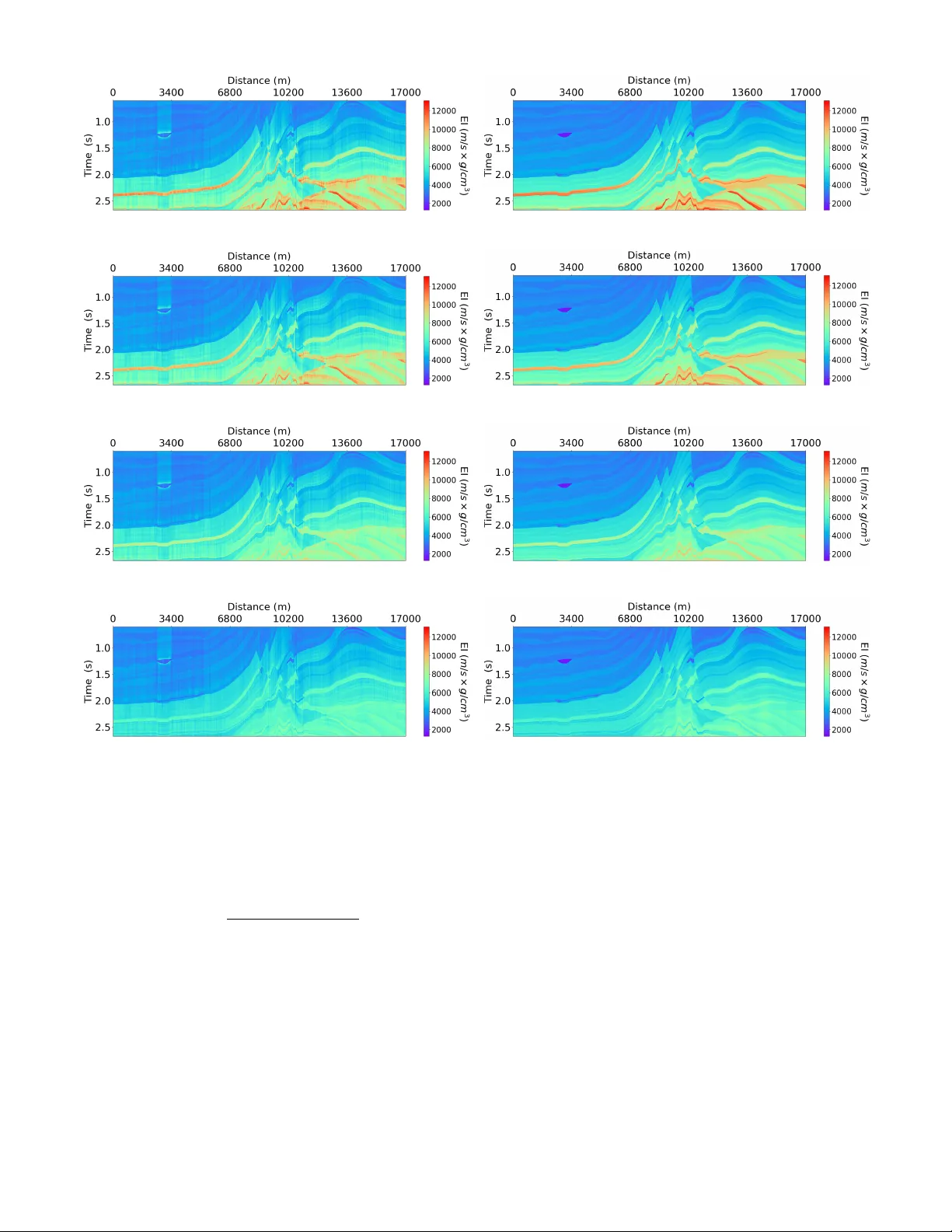
Citation M. Alfarra j and G. AlRegib, (2019), ”Semisupervised sequence mo deling for elas- tic imp edance inv ersion,” Interpr etation 7: SE237-SE249. Review Accepted on: 29 May 2019 Data and Co des [GitHub Link] Bib { @articlealfarraj2019semi, title= { Semi-supervised Sequence Modeling for Elastic Impedance Inversion } , author= { Alfarraj, Motaz and AlRegib, Ghassan } , journal= { Interpretation } , volume= { 7 } , number= { 3 } , pages= { SE237--SE249 } , year= { 2019 } , publisher=Society of Exploration Geophysicists and American Association of Petroleum Geologists } Con tact motaz@gatec h.edu OR alregib@gatech.edu http://ghassanalregib.info/ Semi-sup ervised Sequence Modeling for Elastic Impedance In version 1 Semi-sup ervised Sequence Mo deling for Elastic Imp edance In v ersion Motaz Alfarra j ∗ and Ghassan AlRegib ∗ ABSTRA CT Recen t applications of mac hine learning algorithms in the seismic domain ha ve sho wn great potential in dif- feren t areas suc h as seismic in version and in terpreta- tion. How ev er, suc h algorithms rarely enforce geophys- ical constrain ts; the lac k of whic h might lead to un- desirable results. T o ov ercome this issue, we prop ose a semi-sup ervise d se quenc e mo deling fr amework b ase d on r e curr ent neur al networks for elastic inversion fr om multi-angle seismic data . Sp ecifically , seismic traces and elastic imp edance traces are mo deled as time se- ries. Then, a neural-netw ork-based in version mo del comprising conv olutional and recurren t neural la yers is used to inv ert seismic data for elastic imp edance. The prop osed w orkflow uses w ell-log data to guide the inv er- sion. In addition, it utilizes seismic forward mo deling to regularize the training, and to serv e as a geophysi- cal constraint for the in version. The proposed w orkflo w ac hieves an av erage correlation of 98% b et ween the es- timated and target elastic imp edance using 10 w ell-logs for training on a syn thetic dataset. INTR ODUCTION Seismic in version is a process used to estimate ro ck prop- erties from seismic reflection data. F or example, seismic in version can b e used to infer acoustic impedance (AI) from zero-offset seismic data, whic h in turn is used to es- timate p orosity . AI is the pro duct of P-w av e velocity ( V p ) and bulk density ( ρ ). An extension of AI for multi-angle seismic data is elastic imp edance (EI) (Connolly, 1999). EI is a function of P-w av e v elo city ( V p ), S-w av e v elo city ( V s ), density ( ρ ), and inciden t angle ( θ ). EI reduces to AI when θ = 0 (Whitcombe, 2002), and it utilizes informa- tion from multi-offset/angle seismic data. Th us, in verting ∗ Center for Energy and Geo Pro cessing (CeGP), Georgia In- stitute of T echnology , Atlan ta, GA for EI is a more pow erful to ol for reservoir characterization compared to AI inv ersion. The goal of inv ersion is to infer true mo del parameters ( m ∈ X ) through an indirect set of measurements d ∈ Y . Mathematically , the problem can be formulated as follo ws d = F ( m ) + n, (1) where F : X → Y is a forward op erator, d is the mea- sured data, m is the mo del, and n ∈ Y is a random v ariable that represen ts noise in the measurements. T o estimate the mo del from the measured data, one needs to solv e an inv erse problem. The solution depends on the nature of the forward mo del and observed data. In the case of seismic inv ersion, and due to the non-linearity and heterogeneity of the subsurface, the in verse problem is highly ill-p osed. In order to find a stable solution to an ill-p osed problem, the problem is often regularized by imp osing constraints on the solution space, or by incor- p orating prior knowledge ab out the mo del. A classical approac h to solve inv erse problems is to set up the prob- lem as a Bay esian inference problem, and improv e prior kno wledge b y optimizing for a cost function based on the data likelihoo d, ˆ m = argmin m ∈ X [ H ( F ( m ) , d ) + λ C ( m )] , (2) where ˆ m is the estimated mo del, H : Y × Y → R is an affine transform of the data likelihoo d, C : X → R is a regularization function that incorporates prior kno wledge, and λ ∈ R is regularization parameter that con trols the influence of the regularization function. The solution of equation 2 in seismic in version can b e sough t in a sto c hastic or a deterministic fashion through an optimization routine. In stochastic inv ersion, the out- come is a posterior probability density function; or multi- ple v alid solutions to account for uncertaint y in the data. On the other hand, deterministic inv ersion pro duces an es- timate ( ˆ m ) that maximizes the p osterior probability den- sit y function. The literature of seismic in v ersion (b oth de- terministic and sto chastic) is ric h in v arious metho ds to 2 Alfarra j & AlRegib form ulate, regularize and solve the problem (e.g., (Duijn- dam, 1988a; Do yen, 1988; Duijndam, 1988b; Ulryc h et al., 2001; Buland and Omre, 2003; T aran tola, 2005; Do yen, 2007; Bosc h et al., 2010; Gholami, 2015; Azevedo and Soares, 2017)). Recen tly , there hav e been several successful applications of machine learning and deep learning metho ds to solving in verse problems (Lucas et al., 2018). Moreo ver, mac hine learning and deep learning metho ds hav e b een utilized in the seismic domain for differen t tasks suc h as inv ersion and in terpretation (AlRegib et al., 2018). F or example, seismic in version has been attempted using sup ervised-learning algorithms suc h as support v ector regression (SVR) (Al- Anazi and Gates, 2012), artificial neural net w orks (R¨ oth and T arantola, 1994; Aray a-Polo et al., 2018), committee mo dels (Gholami and Ansari, 2017), conv olutional neu- ral net works (CNNs) (Das et al., 2018), and many other metho ds (Chaki et al., 2015; Y uan and W ang, 2013; Gho- lami and Ansari, 2017; Chaki et al., 2017; Mosser et al., 2018; Chaki et al., 2018). More recently , a sequence- mo deling-based mac hine learning workflo w w as used to es- timate p etrophysical prop erties from seismic data (Alfar- ra j and AlRegib, 2018), which sho wed that recurren t neu- ral net works are sup erior to feed-forw ard neural netw orks in capturing the temp oral dynamics of seismic traces. In general, machine learning algorithms can be used to inv ert seismic data b y learning a non-linear mapping parameterized by Θ ∈ Z ⊆ R n , i.e., F † Θ : Y → X from a set of examples (known as a training dataset) such that: F † Θ ( d ) ≈ m. (3) A key difference b etw een classical in version metho ds and learning-based methods is the outcome. In classi- cal inv ersion, the outcome is a set of mo del parameters (deterministic) or a p osterior probabilit y density func- tion (sto chastic). On the other hand, learning metho ds pro duce a mapping from the measuremen ts domain (seis- mic) to mo del parameters domain (ro ck property). An- other k ey difference betw een the t wo approac hes is their sensitivit y to the initialization of the optimization rou- tine. In classical in version, the initial guess (p osed as a prior mo del) pla ys an imp ortant role in the con vergence of the metho d, and in the final solution. On the other hand, learning-based metho ds are often randomly initial- ized, and prior knowledge is in tegrated into the ob jective function and is inferred by the learning algorithm from the training data. Th us, learning-based inv ersion is less sensitiv e to the initial guess. On the other hand, learning- based inv ersion requires a high-quality training dataset in order to generate reliable results. Nev ertheless, there ha ve b een efforts to o vercome this shortcoming of neural net- w orks and enable them to learn from noisy or unreliable data (Natara jan et al., 2013). There are many challenges, ho wev er, that might preven t mac hine learning algorithms from finding a proper map- ping that can b e generalized for an en tire surv ey area. One of the c hallenges is the lack of data from a given sur- v ey area on whic h an algorithm can be trained. F or this reason, such algorithms m ust hav e a limited num ber of learnable parameters and a go o d regularization method in order to preven t ov er-fitting and to b e able to gener- alize b eyond the training data. Moreov er, applications of mac hine learning on seismic data do not often utilize or enforce a physical mo del that can be used to chec k the v alidit y of their outputs. In other w ords, there is a high dep endence on mac hine learning algorithms to understand the inherent prop erties of the target outputs without ex- plicitly sp ecifying a physical model. Suc h dep endence can lead to undesirable or incorrect results, especially when data is limited. In this w ork, w e prop ose a semi-sup ervised learning w orkflow for elastic imp edance (EI) inv ersion from multi- angle seismic data using sequence mo deling through a com bination of recurren t and con volutional neural net- w orks. The prop osed workflo w learns a non-linear in verse mapping from a training set consisting of w ell-log data and their corresponding seismic data. In addition, the learning is guided and regularized by a forward mo del as often incorp orated in classical inv ersion theory . The rest of this pap er is organized as follows. First, we discuss the form ulation of learning-based seismic inv ersion. Then, we in tro duce recurrent neural netw orks as one of the main comp onen ts in the prop osed workflo w. Next, we discuss the technical details of the prop osed w orkflo w. Then, w e presen t a case study to v alidate the prop osed framework on the Marmousi 2 mo del (Martin et al., 2006) by inv ert- ing for EI using seismic data and 10 well-logs only . PR OBLEM F ORMULA TION Using neural netw orks, one can learn the parameter Θ (in equation 3) in either a sup ervised manner or an unsup er- vised manner (Adler and ¨ Oktem, 2017). In sup ervised learning, the machine learning algorithm is giv en a set of measuremen t-mo del pairs ( d, m ) (e.g., seismic traces and their corresponding prop erty traces from well-logs). Then, the algorithm learns the inv erse mapping by minimizing the following loss function L 1 (Θ) := X i m i ∈S D  m i , F † Θ ( d i )  (4) where S is the set of a v ailable property traces from well- logs, m i is the i th trace in S , d i is the seismic traces cor- resp onding to m i , and D is a distance measure that com- pares the estimated rock prop erty to the true prop erty . Namely , sup ervised mac hine learning algorithms seek a solution that minimizes the inv ersion error ov er the giv en measuremen t-mo del pairs. Note that equation 4 is com- puted only ov er a subset of all traces in the survey . This subset includes the traces for whic h a corresponding prop- ert y trace is av ailable from well-logs. Alternativ ely , the parameters Θ can b e sought in an unsup ervised-learning scheme where the learning algorithm is given a set of measuremen ts ( d ) and a forw ard mo del Semi-sup ervised Sequence Modeling for Elastic Impedance In version 3 F . The algorithm then learns by minimizing the following loss function, L 2 (Θ) := X i D  F  F † Θ ( d i )  , d i  , (5) whic h is computed o ver all seismic traces in the survey . The loss in equation 5 is kno wn as data misfit. It mea- sures the distance b etw een the input seismic traces and the synthesized seismograms from the estimated prop erty traces using the forward mo del. Although sup ervised metho ds hav e b een sho wn to be sup erior to unsup ervised ones in v arious learning tasks (e.g., image segmen tation and ob ject recognition), they often need to b e trained on a large n umber of training examples. In the case of the seismic inv ersion, the lab els (i.e., prop erty traces) are scarce since they come from w ell- logs. Unsup ervised metho ds, on the other hand, do not require labeled data, and th us can b e trained on all av ail- able seismic data only . Ho wev er, unsup e rvised learning do es not integrate well-logs (direct model measurements) in the learning. In this w ork, w e prop ose a semi-sup ervised learning w orkflow for seismic inv ersion that in tegrates b oth well- log data in addition to data misfit in learning the inv erse mo del. F ormally , the los s function of the prop osed semi- sup ervised workflo w is written as L (Θ) := α · L 1 (Θ) | {z } property loss + β · L 2 (Θ) | {z } seismic loss (6) where α, β ∈ R are tuning parameters that gov ern the influence of eac h of the prop erty loss and seismic loss, resp ectiv ely . F or example, if the input seismic data is noisy , or well-log data is corrupted, the v alues of α and β can b e used to limit the role of the corrupted data in the learning pro cess. The prop erty loss is computed o ver the traces for which w e hav e access to mo del measurements (ro c k prop erties) form w ell-logs. The seismic loss , on the other hand, is computed o ver all traces in the survey . The goal of this work is to inv ert for elastic imp edance (EI) using m ulti-offset data using semi-sup ervised sequence mo deling. Hence, ( d ) in the equation 6 is the set of all m ulti-angle traces in the seismic survey , and m is the set of av ailable EI traces from well-logs. Naturally , the size of m is small compared to d . F urthermore, the vertical resolution of EI traces is finer than that of the seismic traces . There are tw o common w ays to mo del traces in a learning paradigm. The first method is to treat each data p oin t in a well-log (in the z -direction) as an indep endent sample and try to inv ert for a giv en ro ck property from the corresp onding m ulti-angle seismic data sample. This metho d fails to capture the long-term temp oral dynamics of seismic traces; that is the dependency betw een a data p oin t at a given depth and the data p oints b efore it and after it. An alternativ e approac h is to treat each trace as a single training sample to incorp orate the temp oral dep endency . Ho wev er, this approac h sev erely limits the amoun t of data from which the algorithm can learn since eac h trace is treated as a single training sample. With a limited amoun t of training data, common machine learn- ing algorithms might fail to generalize b eyond the train- ing data b ecause of their high data requirements. Such a requirement might b e difficult to meet in practical set- tings where the num b er of w ell-logs is limited. In order to remedy this, the prop osed workflo w utilizes sequence mo deling to mo del traces as sequential data via recurren t neural netw orks. RECURRENT NEURAL NETW ORKS Despite the success of feed-forward machine learning meth- o ds, including conv olutional netw orks, multila yer p ercep- trons, and supp ort v ector machines for v arious learning tasks, they hav e their limitations. F eed-forward metho ds ha ve an underlying assumption that data p oints are inde- p enden t, whic h makes them fail in mo deling sequen tially dep enden t data suc h as videos, sp eech signals, and seismic traces. Recurren t neural net w orks (RNN), on the other hand, are a class of artificial neural netw orks that are designed to capture temp oral dynamics of sequen tial data. Un- lik e feed-forward neural net works, RNNs ha ve a hidden state v ariable that can be passed b etw een sequence sam- ples whic h allows them to capture long temporal dep en- dencies in sequential data. RNNs hav e b een utilized to solv e many problems in language mo deling and natural language processing (NLP)(Mikolo v et al., 2010), sp eech and audio processing (Grav es et al., 2013), video pro cess- ing (Ma et al., 2017), p etrophysical prop erty estimation (Alfarra j and AlRegib, 2018), detection of natural earth- quak es (Wiszniowski et al., 2014), and stacking velocity estimation (Biswas et al., 2018). A single lay er feed-forward neural net work pro duces an output y i whic h is a weigh ted sum of input features x i follo wed by an activ ation function (a non-linearit y) like the sigmoid or hyperb olic tangen t functions, i.e. y i = σ ( Wx i + b ), where x i and y i are the input and output feature vectors of the i th sample, resp ectively , σ ( · ) is the activ ation function, W and b are the learnable weigh t matrix and bias v ector, resp ectively . The same equation is applied to all data samples indep endently to pro duce corresp onding outputs. In addition to the affine transformation and the acti- v ation function, RNNs in tro duce a hidden state v ariable that is computed using the curren t input and the hidden state v ariable from the previous step, h ( t ) i = σ  W xh x ( t ) i + W hh h ( t − 1) i + b h  , y ( t ) i = σ  W hy h ( t ) i + b y  (7) where x ( t ) i , y ( t ) i and h ( t ) i , are the input, output, and state v ectors at time step t , resp ectively , W ’s and b ’s are net work weigh ts and bias vectors resp ectively . F or time t = 0, the hidden state v ariable is set to h (0) = 0 . Figure 1 shows a side-b y-side comparison b etw een a feed-forward unit and a recurrent unit. 4 Alfarra j & AlRegib Re c u r r e n t Network Input Output Delay Fe e d - fo r w a rd Network Neural Network h (#$ %) h (#) y (#) x (#) Neural Network y (#) x (#) h (#) State x (#) y (#) Figure 1: An illustration of feed-forw ard and recurren t net works. When RNNs were prop osed in the 1980s, they w ere dif- ficult to train b ecause of the in tro duced dep endency be- t ween data samples that made the gradien ts more difficult to compute. The problem was later solved using back- propagation through time (BPTT) algorithms (W erb os, 1990), whic h turns gradien ts in to long products of terms using the chain rule. Theoretically , RNNs are supp osed to learn long-term dep endencies from their hidden state v ari- able. How ev er, ev en with BPTT, RNNs fail to learn long- term dependencies mainly b ecause the gradien ts tend to v anish for long sequences when backpropagated through time. New RNN architectures hav e b een prop osed to ov er- come the issue of v anishing gradients using gated units. Examples of suc h arc hitectures are Long Short-T erm Mem- ory (LSTM) (Ho c hreiter and Schmidh ub er, 1997) and the recen tly prop osed Gated Recurrent Units (GR U) (Cho et al., 2014). Suc h architectures hav e b een shown to cap- ture long-term dep endency and p erform well for v arious tasks such as mac hine translation and sp eech recognition. In this work, we utilize GR Us in the prop osed inv ersion w orkflow. GR Us supplement the simple RNN describ ed ab o ve by incorp orating reset-gate and up date-gate v ariables which are internal states that are used to ev aluate the long-term dep endency and k eep information from previous times only if they are needed. The forw ard step through a GRU is given b y the following equations, u ( t ) i = sigmoid  W xu x ( t ) i + W y u y ( t − 1) i + b u  r ( t ) i = sigmoid  W xr x ( t ) i + W y r y ( t − 1) i + b r  ˆ y ( t ) i = tanh  W x ˆ y x ( t ) i + b ˆ y 1 + r ( t ) i ◦  W h ˆ y y ( t − 1) i + b ˆ y 2  y ( t ) i = (1 − u ( t ) ) ◦ y ( t − 1) i + u ( t ) ◦ ˆ y ( t ) (8) where u ( t ) i and r ( t ) i are the up date-gate and reset-gate v ectors, resp ectiv ely , ˆ y ( t ) i is the candidate output for the curren t time step, W ’s and b ’s are the learnable parame- ters, and the op erator ◦ is the elemen t-wise pro duct. Note that the GR U in tro duces tw o new state v ariables, up date- gate u and reset-gate r , which con trol the flow of infor- mation from one time step to another, and thus they are able to capture long-term dependency . The output of the GR U at the current time step ( y ( t ) i ) is a w eighted sum of the candidate output for the curren t time step and the output from the previous step. Figure 2 sho ws a G R U net- w ork unfolded through time. Note that all GRUs in an unfolded netw ork share the same W and u parameters. GRU GRU GRU ! " # $% & " # $% '(& " # $% ')& * # $% +(& * # $% & * # $% '(& * # $% ')& ! Figure 2: Gated Recurrent Unit (GRU) unfolded through time. METHODOLOGY Similar to all deep learning metho ds, RNNs require tremen- dous amoun ts of data to train. Given that well-log data is limited in a giv en surv ey area, the num b er of training samples is limited. With suc h limitation, a com bination of regularization tec hniques m ust be used to train a learning- based mo del prop erly and ensure it generalizes b eyond the training dataset (Alfarra j and AlRegib, 2018). In ad- dition, the data shortage limits the num ber of the la yers (and hence parameters) that can b e used in learning-based mo dels. Therefore, using deep er net w orks to capture the highly non-linear in verse mapping from seismic data to EI migh t not b e feasible using sup ervised learning. In this work, we utilize a seismic forward mo del as an- other form of supervision in addition to w ell-log data. Al- though forward mo deling is an essential blo c k in classical seismic in version approaches, it has not b een integrated in to learning-based seismic inv ersion workflo ws. Using a forwar d mo del in a learning-based in version has t wo main adv antages. First, it allows the incorp oration of Semi-sup ervised Sequence Modeling for Elastic Impedance In version 5 geoph ysics into a machine learning paradigm to ensure that the outputs of the netw orks are ob eying the ph ysical la ws. In addition, it allows the algorithm to learn from all traces in the seismic survey without explicitly providing an EI trace (lab el) for each seismic trace. Prop osed w orkflow The in v erse mo del ( F † Θ ) can, in principle, be trained us- ing w ell-log data and their corresponding seismic data only . Ho wev er, as w e hav e discussed earlier, a deep in- v erse mo del requires a large dataset of lab eled data to train prop erly which is not p ossible in a practical setting where the num b er of well-logs is limited. Integrating a forw ard mo del, as commonly done in classical inv ersion w orkflows, allo ws the inv erse mo del to learn from the seis- mic data without requiring their corresp onding property traces, in addition to learning from the few a v ailable prop- ert y traces from well-logs. The ov erall prop osed inv ersion w orkflow is shown in Figure 3. Inver se Model Forward Model Estimated EI Input Seismic Ta r g et E I (from well logs ) Property Loss Seismic Loss Synthe sized Seismic Update Update Figure 3: The proposed semi-sup ervised inv ersion work- flo w. The w orkflow in Figure 3 consists of tw o main mo dules: the in verse mo del ( F † Θ ) with learnable parameters, and a forward mo del ( F ) with no learnable parameters. The prop osed workflo w takes m ulti-angle seismic traces as in- puts, and outputs the b est estimate of the corresp onding EI. Then, the forw ard mo del is used to syn thesize multi- offset seismograms from the estimated EI. The error (data misfit) is computed b et ween the synthesized seismogram and the input seismic traces using the seismic loss . This pro cess is done for all traces in the survey . F urthermore, pr op erty loss is computed b etw een estimated and true EI on traces for whic h we hav e a true EI from well-logs. The parameters of the in verse mo del are adjusted by combin- ing b oth losses as in equation 6 using a gradient-descen t optimization. In this work, w e chose the distance measure ( D ) as the Mean Squared Error (MSE) and α = β = 1. Hence, equation 6 reduces to: L (Θ) = 1 N p X i m i ∈S k m i −F † Θ ( d i ) k 2 2 + 1 N s X i k d i −F ( F † Θ ( d i )) k 2 2 (9) where N s is the total num b er of seismic traces in the surv ey , and N p = |S | is the n umber of a v ailable well- logs. In seismic surveys, N p  N s , therefore, seismic loss is computed ov er many more traces than the property loss. On the other hand, pr op erty loss has access to direct mo del parameters (well-log data). These factors mak e the tw o losses work in collab oration to learn a stable and accurate inv erse mo del. It is imp ortant to note that the c hoice of the forward mo del is critical in the prop osed workflo w for t wo rea- sons. First, the forw ard mo del m ust b e able to synthesize at a sp eed comparable to the sp eed at whic h the inv erse mo del pro cesses data. Since deep learning mo dels, in gen- eral, are capable of pro cessing large amounts of data in a v ery short time with GPU technology , the forward mo del m ust be fast. Second, the prop osed inv erse model, as all other deep learning mo dels, adjusts its parameters accord- ing to the gradien ts with resp ect to a defined loss function, therefore, the forward mo del must b e differentiable in or- der to compute gradients with resp ect to the seismic loss. Therefore, in this work, w e chose a con volutional forw ard mo del due to its simplicity and efficiency to reduce com- putation time. Other c hoices of the forw ard mo del are p ossible as long as they satisfy the t w o conditions stated ab o ve. In v erse Mo del The prop osed inv erse model of the prop osed w orkflow (sho wn in Figure 4) consists of four main submodules. These submo dules are lab eled as se quenc e mo deling , lo c al p attern analysis , upsc aling , and r e gr ession . Each of the four submo dules p erforms a different task in the ov erall in verse mo del. The se quenc e mo deling submo dule models temp oral dy- namics of seismic traces and pro duces features that b est represen t the lo w-frequency conten t of EI. The lo c al p at- tern analysis submo dule extracts lo cal attributes from seismic traces that b est model high-frequency trends of EI trace. The upsc aling submo dule takes the sum of the features produced by the previous modules and upscales them vertically . This mo dule is added based on the as- sumption that seismic data are sampled (v ertically) at a lo wer resolution than that of w ell-log data. Finally , the r e- gr ession submo dule maps the upscaled outputs from fea- tures domain to target domain (i.e., EI). The details of eac h these submo dule are discussed next. Se quenc e Mo deling The se quenc e mo deling submo dule consists of a series of bidirectional Gated Recurren t Units (GRU). Each bidi- rectional GR U computes a state v ariable from future and past predictions and is equiv alent to 2 GR Us where one mo dels the trace from shallow to deep er la yers, and the other mo dels the reverse trace. Assuming eac h m ulti-angle seismic traces ha ve c 1 c hannels (one channel for eac h in- ciden t angle), the First GRU tak es these c 1 c hannels as 6 Alfarra j & AlRegib GRU (in= ! " , out= ! # ) GRU (in= ! # , out= ! # ) Upscaling Loca l P at tern An alysis Input Seismi c ConvBlock (kernel= $ ) (in= ! " , out= ! # ) (dilation= % # ) ConvBlock (kernel= $ ) (in= ! " , out= ! # ) (dilation= % & ) ConvBlock (kernel= $ ) ( in= ! " , out= ! # ) (dilation= % " ) Concatenati on ConvBlock (kernel= $ ) (in= '! # , out= ! # ) (dilation= ( ) GRU (in= ! # , out= )! # ) * * DeconvBl ock (kernel = $ ) (in= )! # , out= ! # ) (stride= + " ) DeconvBl ock (kernel= $ ) (in= ! # , out= ! # ) (stride= + # ) Sequen ce Mode ling Output EI GRU (in= ! # , out= )! # ) Linear (in= ! # , out= ! " ) Re g re s s i o n Figure 4: The inv erse mo del in the prop osed workflo w with generic hyperparameters. The hyperparameters are c hosen based on the data. The num b er of input and output features are denoted by in and out , resp ectively input features and computes c 2 temp oral features based on the temp oral v ariations of the pro cessed traces. The next tw o GRUs p erform a similar task on the outputs of their resp ective preceding GR U. The series of the three GR Us is equiv alent to a 3-lay er deep GR U. Deep er net- w orks are able to model complex input-output relation- ships that shallo w net works migh t not capture. Moreov er, deep GR Us generally produce smooth outputs. Hence, the output of the se quenc e mo deling submo dule is considered as the lo w-frequency trend of EI. L o c al p attern analysis Another submo dule of the inv erse model is the lo c al p at- tern analysis submodule whic h consists of a set of 1-dimensional con volutional blo cks with different dilation factors in par- allel. The output features of eac h of the parallel con- v olutional blo cks are then com bined using another con- v olutional blo ck. Dilation refers to the spacing b et ween con volution kernel p oints in the con volutional la yers (Y u and Koltun, 2015). Multiple dilation factors of the kernel extract m ultiscale features by incorp orating information from trace samples that are direct neigh b ors to a refer- ence sample (i.e., the cen ter sample), in addition to the samples that are further from it. An illustration of dilated con volution is shown in Figure 5 for a conv olution k ernel of size 5 and dilation factors dilation = 1 , 2 and 3. A con volutional blo ck ( ConvBlo ck ) consists of a conv o- lutional lay er follow ed b y group normalization (W u and He, 2018) and an activ ation function. Group normaliza- tion scales divides the output of the con volutional la yers in to groups, and normalizes eac h group using a learned Dilation = 1 Dilation = 2 Dilation = 3 Convolution k ernel point Center sample Figure 5: An illustration of dilated con volution for multi- scale feature extraction (k ernel size = 5, dilation factors dilation = 1 , 2 and 3). mean and standard deviation. They hav e been sho wn to reduce cov ariant shift in the learned features and speed up the learning. In addition, activ ation functions are one of the building blo cks of any neural net work. They are a source of non-linearity that allow the neural netw orks to approximate highly non-linear functions. In this work, w e chose the h yp erb olic tangen t function as the activ ation function. Con volutional lay ers op erate on small windows of the input trace due to their small kernel sizes. Therefore, they capture high-frequency con tent. Since conv olutional la yers do not hav e a state v ariable lik e recurrent lay ers to serv e as a memory , they do po orly in estimating the low- frequency conten t. The outputs of the lo c al p attern anal- ysis submo dule are of very similar dimensions of those of the se quenc e mo deling submodule. Hence, the outputs of the tw o mo dules are added to obtain a full-band frequency Semi-sup ervised Sequence Modeling for Elastic Impedance In version 7 con tent. upsc aling Seismic data is sampled at a low er rate than that of w ell- logs data. The role of the upsc aling submo dule is to com- p ensate for this resolution mismatch. This submo dule consists of t wo Deconv olutional Blo cks with different ker- nel stride. The stride controls the factor by whic h the inputs are upscaled. A stride of ( s = 2) deconv olutional blo c k pro duces an output that has twice the num b er of the input samples (vertically). Decon volutional lay ers (also kno wn as transposed con- v olutional or fractionally-strided con volutional la yers) are upscaling mo dules with learnable kernel parameters un- lik e classical in terp olation methods with fixed kernel pa- rameters (e.g., linear interpolation). They learn k ernel parameters from b oth feature and local spatial/temp oral domain. They ha ve b een used for v arious applications lik e semantic segmentation and seismic structure lab eling (Noh et al., 2015; Alaudah et al., 2018). Decon volutional blocks in Figure 4 ha v e a similar struc- ture as the conv olutional blo cks introduced earlier. They are a series of decon volutional la yer follow ed by a group normalization mo dule and an activ ation function. R e gr ession The final submodule in the in verse mo del is the r e gr es- sion submo dule whic h consists of a GR U follo wed b y a linear mapping lay er (fully-connected la yer). Its role is to regress the extracted features from the other mo dules to the target domain (EI domain). The GRU in this mod- ule is a simple 1-la yer GRU that augmen ts the upscaled outputs using global temp oral features. Finally , a linear affine transformation lay er (fully-connected la yer) takes the output features from the GR U and maps them to the same n umber of features in the target domain, which is, in this case, the num b er of incident angles in the target EI trace. F orw ard Mo del F orw ard mo deling is the pro cess of synthesizing seismo- grams from elastic prop erties of the earth (i.e., P-w av e v elo city , S-wa ve velocity , and density) or from a function of the elastic properties such as EI. In this w ork, and since w e are in verting for EI, we used a forward mo del that takes EI as an input, and outputs a corresp onding seismogram. EI was proposed by Connolly (1999) and later normalized b y Whitcom b e (2002). It is based on the Aki-Richards appro ximation for Zo eppritz equations (Aki and Ric hards, 1980). The Aki-Ric hards approximation incorporates am- plitude v ariations with offset/angle (A VO/A V A) based on the changes of elastic prop erties and the incident angle. The forw ard model adopted in this work uses Connolly’s form ulation to compute the reflection coefficients from E I for different inciden t angles θ as follows: RC ( t, θ ) = 1 2 E I ( t + ∆ t, θ ) − E I ( t, θ ) E I ( t + ∆ t, θ ) + E I ( t, θ ) , (10) where ∆ t is the time step, and E I ( t, θ ) is the elastic imp edance at time t and inciden t angle θ . EI in equation 10 refers to the normalized elastic imp edance proposed b y Whitcombe (2002) which is computed from the elastic prop erties as follows: E I ( t, θ ) = V p 0 ρ 0  V p ( t ) V p 0  a  V s ( t ) V s 0  b  ρ ( t ) ρ 0  c , (11) where, a = 1 + tan 2 θ b = 4 K sin 2 θ c = 1 − 4 K sin 2 θ K = V 2 s / V 2 p and V p , V s and ρ are P-w av e velocity , S-wa ve velocity , and densit y , resp ectively , and V p 0 , V s 0 and ρ 0 are their resp ec- tiv e a verages ov er the training sample (i.e., well-logs). It is w orth noting that the Aki-Richard’s appro ximation of the elastic imp edance is only v alid for inciden t angles that are less than 35 ◦ . Th us, in the case study , we only consider v alid angles for this approximation. The seismograms are then generated b y con volving RC ( t, θ ) with a w av elet w ( t ), i.e., S ( t, θ ) = w ( t ) ∗ RC ( t, θ ) , (12) where ∗ is the linear con volution operator, and S ( t, θ ) is the syn thesized seismogram. Thus, the forw ard model uti- lized in this w ork is a 1-dimensional con volutional forw ard mo del that synthesized seismograms from EI traces. CASE STUD Y ON MARMOUSI 2 MODEL In order to v alidate the proposed algorithm, we chose Mar- mousi 2 mo del as a case study . Marmousi 2 mo del is an elastic extension of the original Marmousi syn thetic model that has b een used for numerous studies in geophysics for v arious applications including seismic inv ersion, seismic mo deling, seismic imaging, and A V O analysis. T he mo del spans 17 km in width and 3.5 km in depth with a v erti- cal resolution of 1.25 m. The details of the mo del can b e found in Martin et al. (2006). In this work, w e used the elastic mo del (conv erted to time) to generate EI and seismic data to train the mo del. The details of the dataset generation are discussed in the next section. The prop osed w orkflow is trained using all seismic traces in Marmousi 2 in addition to a few EI traces (training traces). The workflo w is then used to inv ert for EI on the entire Marmousi. Since the full elastic model is a v ailable, we compare our EI inv ersion with the true EI quan titatively . Dataset Generation W e used the elastic mo del of Marmousi 2 to generate EI for 4 incident angles θ = 0 ◦ ,10 ◦ ,20 ◦ , and 30 ◦ . Thus, in Figure 4, c 1 = 4 which represents the n umber of c hannels 8 Alfarra j & AlRegib in the input traces. Multi-angle seismic data (a total of N s = 2720 traces) is then generated from EI using the forw ard model with Ormsby wa v elet (5-10-60-80 Hz) fol- lo wing the synthesis pro cedure in (Martin et al., 2006). The seismic traces are then downsampled (in time) by a factor of 6 to sim ulate resolution difference b etw een seis- mic and well-log data. Finally , a 15 db white Gaussian noise is added to assess the robustness of the prop osed w orkflow to noise. T o train the prop osed in version workflo w, w e c hose 10 ev enly-spaced traces for training ( N p = 10) as sho wn in Figure 6. W e assume we ha ve access to b oth EI and seis- mic data for the training traces. F or all other traces in the surv ey , we assume w e ha ve access to seismic data only . Al- though using more EI traces for training w ould improv e the inv ersion, in this work we use only 10 EI traces for training to sim ulate well-log data in a practical setting. Figure 6: The training EI traces ov erlaid on the zero-offset seismic section. T raining The Inv erse Mo del First, the in verse mo del (neural netw ork) is initialized with random parameters. Then, randomly c hosen seismic traces in addition to the seismic traces for which w e ha ve EI traces in the training dataset are inputted to the inv erse mo del to get a corresponding set of EI traces. The forw ard mo del is then used to synthesize seismograms from the es- timated EI. Seismic loss is computed as the MSE betw een the syn thesized seismic and the input seismic. Moreov er, pr op erty loss is computed as the MSE b etw een the pre- dicted EI and the true EI trace on the training traces only . The total loss is computed as the sum of the tw o losses. Then, the gradien ts of the total loss are computed, and the parameters of the inv erse mo del are up dated accordingly . The pro cess is rep eated until con vergence. Figure 4 shows the inv erse mo del with no given hyper- parameters to ensure its generalizabilit y for data other than the data used in this case study . These hyperpa- rameters are { c 1 , c 2 , s 1 , s 2 , d 1 , d 2 , k } which are parameters of the inv ersion mo del that need to be set rather than learned. Some of these h yp erparameters are completely dictated by the data. F or example, c 1 whic h is the n um- b er of inputs c hannels must be chosen as the num b er of inciden t angles of the data. Also, s 1 , s 2 m ust b e chosen suc h that s 1 × s 2 is equal to the resolution mismatch fac- tor b et ween seismic and EI data. In this case study , w e set c 1 = 4, s 1 = 3, and s 2 = 2. The rest of the hyper- parameters are chosen b y analyzing the data and trying differen t v alues and testing the p erformance on a v alida- tion dataset using cross-v alidation. In this case study , we c ho ose c 2 = 8, k = 5, d 1 = 1, d 2 = 3, and d 3 = 6. Results and Discussion Figure 7 sho ws estimated EI and true EI for the entire sec- tion for all four incident angles. Figure 8 sho ws the abso- lute difference b etw een the true and estimated EI. The fig- ures indicate that the proposed w orkflow estimates EI ac- curately for most parts of the section with a visible lateral jitter. Jitter effect is exp ected since the prop osed work- flo w is based on 1-dimensional sequence mo deling with no explicit spatial constrain ts as often done in classical in- v ersion methods. F urthermore, the noise in the seismic data reduces the similarit y betw een neigh b oring seismic traces, which can also cause suc h jitter. The sho wn sec- tions are the direct output of the inv ersion workflo w with no p ost-pro cessing which can reduce such artifacts. Figure 9 sho ws tw o selected traces from the section that were not in the training dataset ( x = 3200 m and x = 8500 m). The trace at x = 3200 passes through an anomaly (Gas-c harged sand channel) represented b y an isolated and sudden transition in EI at 1 . 25 seconds. This anomaly causes the in verse mo del to incorrectly estimate EI. Since our workflo w is based on bidirectional sequence mo deling, w e expect the error to propagate to nearb y sam- ples in b oth directions. How ever, the algorithm quickly reco vers a go o d estimate for deep er and shallo wer sam- ples of the trace. This quick reco very is mainly due to the reset-gate v ariable in the GRU that limits the propagation of suc h errors in sequen tial data estimation. F urthermore, the trace at x = 8500 passes through most lay ers in the section which makes it a challenging trace to in vert. The estimated EI at x = 8500 follo ws the trends in true EI trace, including the thin la yers. F urthermore, we sho w scatter plots of the estimated and true EI for all inciden t angles in Figure 10. The shaded regions in the figure include all p oin ts that are within one standard deviation of the true EI ( σ EI ). The scatter plots sho w a linear correlation b etw een the estimated and true EI with the ma jority of the estimated samples within ± σ EI from the true EI. T o ev aluate the performance of the prop osed workflo w quan titatively , w e use tw o metrics that are commonly used for regression analysis. Namely , Pearson correlation co ef- ficien t (PCC), and coefficient of determination ( r 2 ). PCC is defined as: PCC = 1 T 1 σ x σ ˆ x T − 1 X t =0 [ x ( t ) − µ x ] [ ˆ x ( t ) − µ ˆ x ] , (13) where x and ˆ x are the target trace and the estimated trace, resp ectively , and µ and σ are mean and standard deviation, resp ectively . PCC is a measure of the linear correlation b etw een the estimated and target traces. It is commonly used to measure the o verall fit betw een the t wo traces with no regard to the individual v alues. On Semi-sup ervised Sequence Modeling for Elastic Impedance In version 9 (a) Estimated EI ( θ = 0 ◦ ) (b) T rue EI ( θ = 0 ◦ ) (c) Estimated EI ( θ = 10 ◦ ) (d) T rue EI ( θ = 10 ◦ ) (e) Estimated EI ( θ = 20 ◦ ) (f ) T rue EI ( θ = 20 ◦ ) (g) Estimated EI ( θ = 30 ◦ ) (h) T rue EI ( θ = 30 ◦ ) Figure 7: Estimated EI and true EI for Marmousi 2 mo del. the other hand, r 2 is a go o dness-of-fit measure, where it tak es in to accoun t the mean squared error b et ween the t wo traces. The coefficient of determination ( r 2 ) is defined as: r 2 = 1 − P T − 1 i =0 [ x ( t ) − ˆ x ( t )] 2 P T − 1 i =0 [ x ( t ) − µ x ] 2 (14) In addition, w e used Structural Similarity (SSIM) (W ang et al., 2004) to assess the quality of the estimated EI sec- tion from an image p oint of view. SSIM ev aluates the similarit y of t w o images from local statistics (on lo cal win- do ws) using the following equation: SSIM( X , ˆ X ) = [ l ( x , ˆ x )] α · [ c ( x , ˆ x )] β · [ s ( x , ˆ x )] γ , (15) where x and ˆ x are patches from estimated and target image, respectively . l ( x , y ), c ( x , ˆ x ), and s ( x , ˆ x ) are lu- minance, con trast and structure comparison functions re- sp ectiv ely . α > 0, β > 0, γ > 0 are constants chosen to adjust the influence of the each of three terms. F rom SSIM, a single similarit y v alue, denoted as M-SSIM, can b e computed by taking the mean of all SSIM scores for all lo cal windows. The quantitativ e results are summarized in T able 1. It is eviden t that the estimated EI captures the o verall trend of true EI (av erage PCC ≈ 98%, av erage r 2 ≈ 94%). The a verage r 2 score is low er than PCC since it is more sensi- tiv e to the residual sum of squares rather than the ov erall trend. Note that PCC and r 2 compute scores o ver indi- vidual traces, then the final score (for eac h inciden t angle) is computed by av eraging across all traces. On the other hand, M-SSIM is computed ov er the 2D section (image) whic h takes b oth lateral and vertical v ariations into ac- coun t. 10 Alfarra j & AlRegib (a) θ = 0 ◦ (b) θ = 10 ◦ (c) θ = 20 ◦ (d) θ = 30 ◦ Figure 8: Absolute difference b etw een T rue EI and estimate EI for all inciden t angles. (a) x = 3300 m (b) x = 8500 m Figure 9: Selected EI trace. Estimate EI is shown in red, and true EI is sho wn in black. F urthermore, w e quantify the contribution of each of the tw o terms in the loss function in equation (6) by com- paring the inv ersion results for different v alues of α and β . The av erage results are rep orted in T able 2. When α = 0 and β = 1 (unsup ervised learning), the in verse mo del is learned completely from the seism ic data without in tegrating the well-logs. Thus, the results are the w orst out of three schemes. Note that the p erformance of the unsup ervised learning scheme could b e improv ed by using an initial smooth model and by enforcing some con- strain ts on the in version as often doe in classical in v ersion. Moreo ver, when α = 1 and β = 0 (supervised learning), Semi-sup ervised Sequence Modeling for Elastic Impedance In version 11 (a) θ = 0 ◦ (b) θ = 10 ◦ (c) θ = 20 ◦ (d) θ = 30 ◦ Figure 10: Scatter plots of the estimated and true EI for differen t v alues of θ . The shaded regions include all points that are within ± σ EI of the true EI. T able 1: Quan titative ev aluation of the prop osed w orkflow on Marmousi 2. Angle Metric PCC r 2 M-SSIM θ = 0 ◦ 0.98 0.95 0.92 θ = 10 ◦ 0.98 0.95 0.92 θ = 20 ◦ 0.98 0.95 0.92 θ = 30 ◦ 0.98 0.92 0.92 Av erage 0.98 0.94 0.92 the in version workflo w learns from only 10 seismic traces and their corresp onding EI traces from well-logs. Thus, it is exp ected that it results in b etter inv ersion compared to the unsupervised scheme. Ho wev er, training a deep in verse model in a sup ervised learning scheme requires hea vy regularization and careful selection of the train- ing parameters. In addition, the learned in verse mo del migh t not generalize well beyond training data. Finally , when α = β = 1 (semi-sup ervised learning), the inv erse mo del is learned from all seismic data in addition to 10 EI traces from well-logs. Hence, the semi-sup ervised learn- ing scheme impro ves the p erformance and regularizes the learning. Figure 11(a) sho ws the distribution of PCC of the es- timated EI with resp ect to the true EI for all traces in Marmousi 2 model. The figure shows that the estimated EI correlates very well with the true EI, with the ma jor- it y of PCC v alues b etw een [0 . 9 − 1], and a spik e near 1. Similarit y , Figure 11(b) shows the distribution of r 2 v al- ues, with a wider distribution than that of PCC. This is mainly due to the fact that P C C is defined to b e in the range [0 , 1] and r 2 is in the range ( −∞ , 1]. In addition, r 2 is a more strict metric than PCC as it factors in the MSE b et ween the estimated EI and true EI. Figure 11(c) shows the distribution of lo cal SSIM scores ov er the entire sec- tion, with the ma jority of the scores in the range [0 . 8 , 1] indicating that the estimated EI is structurally similar to the true EI from an image p oint of view. (a) Distribution of PCC v alues (b) Distribution of r 2 v alues (c) Distribution of SSIM v alues Figure 11: The distribution of P earson correlation co ef- ficien t (PCC), and co efficien t of determination ( r 2 ), and SSIM v alues on Marmousi 2. Implemen tation The prop osed workflo w was implemented in Python us- ing PyT orch deep learning library (Paszk e et al., 2017). F or optimization, we used Adam (Kingma and Ba, 2014) whic h is a gradient-based sto c hastic optimization tech- nique with adaptiv e learning rate that was designed specif- ically for training deep neural netw orks. The codes w ere run on a PC with Intel i7 Quad-Core CPU, and a single Nvidia GeF orce GTX 1080 Ti GPU. The run time of 500 12 Alfarra j & AlRegib T able 2: Quantitativ e ev aluation of the sensitivity of the loss function with resp ect to its tw o terms. Unsup ervised : learning from all seismic traces in the section, Sup ervised : learning from 10 seismic traces and their corresp onding EI traces, Semi-supervised : learning from all seismic data in the section in addition to 10 seismic traces and their corresp onding EI traces T raining Sc heme Metric PCC r 2 M-SSIM Unsup ervised ( α = 0 , β = 1) 0.33 -0.45 0.77 Sup ervised ( α = 1 , β = 0) 0.96 0.88 0.87 Semi-sup ervised ( α = 1 , β = 1) 0.98 0.94 0.92 iterations of the GPU-accelerated algorithm was 2 min- utes. Figure 12 shows the con vergence b ehavior of the prop osed w orkflow ov er 500 training iterations. The y- axis sho ws the total loss o ver the training dataset which is computed as in equation 9 except for an additional normalization factor that is equal to the num b er of time samples p er trace. Note that the loss is also computed o ver normalized traces after subtracting the mean v alue and dividing by the standard deviation to ensure faster con vergence of the inv ersion w orkflow as often done for deep learning models. The prop osed w orkflow con v erges in about 300 iterations. How ev er, the loss con tinues to de- crease slightly . The training was terminated at after 500 iterations to a void ov er-fitting to the training dataset. Figure 12: T raining learning curve showing the loss func- tion v alue ov er 500 iterations. The efficiency of the prop osed workflo w is due to the use of 1-dimensional mo deling. In addition, Marmousi 2 is a relativ ely small mo del with 2720 traces only . Ho wev er, the computation time of the prop osed workflo w will scale linearly with the num b er of traces in the dataset. The co de used to repro duce the results rep orted in this man uscript is publicly av ailable on GitHub [ link to co de] . CONCLUSIONS In this work, w e proposed an inno v ativ e semi-sup ervised mac hine learning workflo w for elastic imp edance in version from multi-angle seismic data using recurrent neural net- w orks. The prop osed workflo w was v alidated on the Mar- mousi 2 mo del. Although the training w as carried out on a small num b er of EI traces for training, the prop osed w orkflow was able to estimate EI with an a verage corre- lation of 98%. F urthermore, the applications of the pro- p osed workflo w are not limited to EI in v ersion; it can be easily extended to p erform full elastic inv ersion as w ell as prop ert y estimation for reservoir c haracterization. A CKNOWLEDGMENT This work is supp orted by the Center for Energy and Geo Processing (CeGP) at Georgia Institute of T echnol- ogy and King F ahd Universit y of Petroleum and Minerals (KFUPM). REFERENCES Adler, J., and O. ¨ Oktem, 2017, Solving ill-p osed inv erse problems using iterativ e deep neural net w orks: In verse Problems, 33 , 124007. Aki, K., and P . Ric hards, 1980, Quantitativ e seismology , v ol. 2. Al-Anazi, A., and I. Gates, 2012, Support v ector regres- sion to predict porosity and permeability: effect of sam- ple size: Computers & Geosciences, 39 , 64–76. Alaudah, Y., S. Gao, and G. AlRegib, 2018, Learning to lab el seismic structures with deconv olution netw orks and weak labels, in SEG T echnical Program Expanded Abstracts 2018: So ciety of Exploration Geophysicists, 2121–2125. Alfarra j, M., and G. AlRegib, 2018, Petroph ysical prop- ert y estimation from seismic data using recurren t neu- ral netw orks, in SEG T echnical Program Expanded Abstracts 2018: So ciety of Exploration Geophysicists, 2141–2146. AlRegib, G., M. Deric he, Z. Long, H. Di, Z. W ang, Y. Alaudah, M. A. Shafiq, and M. Alfarra j, 2018, Subsur- face structure analysis using computational interpreta- tion and learning: A visual signal pro cessing p ersp ec- tiv e: IEEE Signal Pro cessing Magazine, 35 , 82–98. Ara ya-P olo, M., J. Jennings, A. Adler, and T. Dahlke, 2018, Deep-learning tomography: The Leading Edge, 37 , 58–66. Azev edo, L., and A. Soares, 2017, Geostatistical metho ds for reservoir geoph ysics: Springer. Bisw as, R., A. V assiliou, R. Stromberg, and M. K. Sen, 2018, Stacking velocity estimation using recurren t neu- ral netw ork, in SEG T echnical Program Expanded Ab- Semi-sup ervised Sequence Modeling for Elastic Impedance In version 13 stracts 2018: So ciety of Exploration Geophysicists, 2241–2245. Bosc h, M., T. Muk erji, and E. F. Gonzalez, 2010, Seismic in version for reservoir prop erties com bining statistical ro c k physics and geostatistics: A review: Geoph ysics, 75 , 75A165–75A176. Buland, A., and H. Omre, 2003, Ba yesian linearized av o in version: Geophysics, 68 , 185–198. Chaki, S., A. Routra y , and W. K. Mohant y , 2015, A nov el prepro cessing scheme to impro ve the prediction of sand fraction from seismic attributes using neural netw orks: IEEE Journal of Selected T opics in Applied Earth Ob- serv ations and Remote Sensing, 8 , 1808–1820. ——–, 2017, A diffusion filter based sc heme to denoise seismic attributes and impro ve predicted porosity v ol- ume: IEEE Journal of Selected T opics in Applied Earth Observ ations and Remote Sensing, 10 , 5265–5274. ——–, 2018, W ell-log and seismic data in tegration for reserv oir characterization: A signal pro cessing and mac hine-learning p ersp ective: IEEE Signal Pro cessing Magazine, 35 , 72–81. Cho, K., B. V an Merri¨ enbo er, D. Bahdanau, and Y. Ben- gio, 2014, On the prop erties of neural machine trans- lation: Encoder-deco der approaches: arXiv preprint Connolly , P ., 1999, Elastic impedance: The Leading Edge, 18 , 438–452. Das, V., A. Pollac k, U. W ollner, and T. Mukerji, 2018, Con volutional neural net work for seismic imp edance in version, in SEG T echnical Program Expanded Ab- stracts 2018: So ciety of Exploration Geophysicists, 2071–2075. Do yen, P ., 2007, Seismic reservoir c haracterization: An earth mo delling p ersp ectiv e: EA GE publications Houten, 2 . Do yen, P . M., 1988, Porosit y from seismic data: A geo- statistical approach: Geophysics, 53 , 1263–1275. Duijndam, A., 1988a, Bay esian estimation in seismic in- v ersion. part i: Principles: Geophysical Prospecting, 36 , 878–898. ——–, 1988b, Bay esian estimation in seismic in version. part ii: Uncertain ty analysis: Geoph ysical Prospecting, 36 , 899–918. Gholami, A., 2015, Nonlinear multic hannel imp edance in- v ersion by total-v ariation regularization: Geophysics, 80 , R217–R224. Gholami, A., and H. R. Ansari, 2017, Estimation of p oros- it y from seismic attributes using a committee mo del with bat-inspired optimization algorithm: Journal of P etroleum Science and Engineering, 152 , 238–249. Gra ves, A., A.-r. Mohamed, and G. Hinton, 2013, Sp eec h recognition with deep recurren t neural netw orks: Acoustics, speech and signal processing (ICASSP), 2013 IEEE international conference on, IEEE, 6645–6649. Ho c hreiter, S., and J. Schmidh ub er, 1997, LSTM can solv e hard long time lag problems: Adv ances in neural infor- mation pro cessing systems, 473–479. Kingma, D. P ., and J. Ba, 2014, Adam: A metho d for sto c hastic optimization: arXiv preprint Lucas, A., M. Iliadis, R. Molina, and A. K. Katsaggelos, 2018, Using deep neural net works for in verse problems in imaging: b eyond analytical metho ds: IEEE Signal Pro cessing Magazine, 35 , 20–36. Ma, C.-Y., M.-H. Chen, Z. Kira, and G. AlRegib, 2017, TS-LSTM and temp oral-inception: Exploiting spa- tiotemp oral dynamics for activity recognition: arXiv preprin t Martin, G. S., R. Wiley , and K. J. Marfurt, 2006, Mar- mousi2: An elastic upgrade for marmousi: The Leading Edge, 25 , 156–166. Mik olov, T., M. Karafi´ at, L. Burget, J. ˇ Cerno c k ` y, and S. Kh udanpur, 2010, Recurren t neural net work based lan- guage mo del: Presented at the Elev enth Ann ual Con- ference of the International Sp eech Comm unication As- so ciation. Mosser, L., W. Kimman, J. Dramsch, S. Purves, A. De la F uen te Brice ˜ no, and G. Ganssle, 2018, Rapid seismic domain transfer: Seismic velocity inv ersion and mo del- ing using deep generativ e neural netw orks: Presen ted at the 80th EAGE Conference and Exhibition 2018. Natara jan, N., I. S. Dhillon, P . K. Ra vikumar, and A. T ew ari, 2013, Learning with noisy lab els: Adv ances in neural information pro cessing systems, 1196–1204. Noh, H., S. Hong, and B. Han, 2015, Learning deconv olu- tion net work for seman tic segmen tation: Pro ceedings of the IEEE international conference on computer vision, 1520–1528. P aszke, A., S. Gross, S. Chintala, G. Chanan, E. Y ang, Z. DeVito, Z. Lin, A. Desmaison, L. An tiga, and A. Lerer, 2017, Automatic differen tiation in pytorc h: Presen ted at the NIPS-W. R¨ oth, G., and A. T arantola, 1994, Neural netw orks and in version of seismic data: Journal of Geophysical Re- searc h: Solid Earth, 99 , 6753–6768. T aran tola, A., 2005, Inv erse problem theory and methods for mo del parameter estimation: siam, 89 . Ulryc h, T. J., M. D. Sacchi, and A. W o o dbury , 2001, A ba yes tour of inv ersion: A tutorial: Geophysics, 66 , 55–69. W ang, Z., A. C. Bovik, H. R. Sheikh, E. P . Simoncelli, et al., 2004, Image quality assessment: from error vis- ibilit y to structural similarity: IEEE transactions on image pro cessing, 13 , 600–612. W erb os, P . J., 1990, Bac kpropagation through time: what it do es and how to do it: Pro ceedings of the IEEE, 78 , 1550–1560. Whitcom b e, D. N., 2002, Elastic imp edance normaliza- tion: Geophysics, 67 , 60–62. Wisznio wski, J., B. M. Plesiewicz, and J. T ro jano wski, 2014, Application of real time recurrent neural net work for detection of small natural earthquak es in poland: Acta Geophysica, 62 , 469–485. W u, Y., and K. He, 2018, Group normalization: Pro ceed- 14 Alfarra j & AlRegib ings of the Europ ean Conference on Computer Vision (ECCV), 3–19. Y u, F., and V. Koltun, 2015, Multi-scale context ag- gregation by dilated conv olutions: arXiv preprint Y uan, S., and S. W ang, 2013, Spectral sparse Ba yesian learning reflectivity in version: Geoph ysical Prosp ect- ing, 61 , 735–746.