Stochastic differential theory of cricket

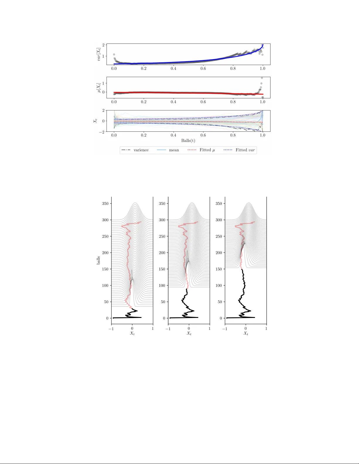
Sto c hastic differen tial theory of cric k et San tosh Kumar Radha Dep artment of physics *Case Western R eserve University Abstract A new formalism for analyzing the progression of crick et game using Sto c hastic differen tial equa- tion (SDE) is in tro duced. This theory enables a quan titative wa y of represen ting every team using three key v ariables which ha v e physical meaning asso ciated with them. This is in con trast with the traditional system of rating/ranking teams based on com bination of differen t statical cum ulants. F ur- ther more, using this formalism, a new method to calculate the winning probabilit y as a progression of n um b er of balls is giv en. Keywor ds: Sto c hastic Differen tial Equation, Cric ket, Sports, Math, Ph ysics 1. In tro duction Sp orts, as a social en tertainer exists b ecause of the unpredictable nature of its outcome. More recen tly , the w orld cup final cric ket match b et w een England and New Zealand serves as a prime example of this unpredictability . Ev en when one team is hea vily adv an tageous, there is a chance that the other team will win and that likelihoo d v aries by the particular sp ort as w ell as the teams in volv ed. There ha v e been man y studies sho wing that unpredictabilit y is an una v oidable fact of sports [ 1 ], despite which there has b een numerous attempts at predicting the outcome of sp orts [ 5 ]. Though differen t, there has b een considerable efforts directed to wards predicting the future of other fields including financial mark ets [ 4 ], arts and entertainmen t a w ard ev ents [ 6 ], and p olitics [ 7 ]. There has b een a wide range of statistical analysis p erformed on sp orts, primarily baseball and fo otball[ 8 , 2 , 3 ] but v ery few ha ve b een applied to understand crick et. Complex system analysis[ 9 ], mac hine learning mo dels[ 10 , 12 ] and v arious statical data analysis[ 13 , 14 , 15 , 16 , 17 ] hav e b een used in previous studies to describ e and analyze crick et. In this pap er, we hav e come up with statistical sto c hastic mo dels that describ e crick et. The adv antage of using DEs to mo del even ts is that, it leads to making physically realistic assumptions on the sp ort whic h leads to having v ariables in SDEs that ha ve describable meaning attached to it. W e introduce the concept of using SDE for the game of crick et using a very rudimen tary mo del in subsection 2.1 . This mo del has a very basic analytic form and introduces the ideas b ehind this pap er. Since SDE models the sp ort at its fundamen tal level, one can then use these mo dels as basis for adding more terms that tak e in to account the complexities of the game. As a example, in subsection 2.2 w e pro ceed to add sligh t mo difications to the same mo del to describ e in b etter the concept “wickets Email addr ess: srr70@case.edu (San tosh Kumar Radha) URL: www.santoshkumarradha.me (San tosh Kumar Radha) in hand” . Example uses of these mo dels are sho wn for a particular historic crick et game b et ween India-Srilanka . Finally a more sophisticated mo del that describ es the exact dynamics b et w een the t wo teams is developed and shown in subsection 2.3 . 2. F ormalism 2.1. Mo del 1 Cen tral Idea b ehind this entire theory relies on using the v ariable X defined as the difference b et w een Required run rate p er ball ( RR ) and Net run rate p er ball ( N R ) 1 giv en b y X ( t ) = N R ( t ) − RR ( t ) (1) t ∈ [0 , T ] Here, T refers to the total num b er of balls in the game. Since w e are using RR to define the v ariable, the mo del can b e used only after the first innings of the game. This v ariable X ( t ) is an quan tity that is typically in b etw een ± 3 and more negative the n umber is, the more the team batting in the second innings is lo osing. Figure 1 sho ws a typical plot X ( t ) for an ODI game tak en from a match b etw een India and Srilank a. Figure 1: t ypical X ( t ) from a cric ket match. Here it is sho wn for an ODI game and hence T = 300. Blue p oin ts represen t ev ery 4 th ball and red line, the entire game. One can write the distribution of the lead of one team ov er an other team ( X ( t )) at any p oin t in the game as a w einner pro cess. Let ( W t ) t ≥ 0+ denotes a standard Brownian motion satisfying • W 0 = 0 • With probability 1, the function t → W t is contin uous in t • The pro cess ( W t ) t ≥ 0+ has stationary , indep enden t increments • The increment W t + s − W s = N (0 , t ) then the equation X ( t ) = µt + σ W t ≈ N ( µt, σ 2 t ) (2) 1 RR (Required run rate) is defined as (runs sc or e d in first innings - runs til l curr ent b al l)/No. of b al ls left in this innings NR (Net run rate p er ball) is defined as the curr ent sc or e in se c ond innings/numb er of b al ls playe d 2 can b e used to describ e the distribution of X ( t ) with µ and σ generalizing the winner pro cess giving raise to mean and v ariance of the resulting normal distribution. Figure 3 shows actual data fitted to this kind of pro cess. Though the fit does not seem to b e perfect, this can be used to illustrate the idea b ehind this formalism (Better mo del is developed later in the pap er ). µ and σ , in sto chastic terms represent the drift and volatilit y in the pro cess. This immediately shows the h uge adv antage of mo deling the sp ort using this type of pro cess. µ ’s of eac h team would indicate quan titatively , the adv an tage(disadv antage) the team 1(2) has ov er team 2(1). σ v ariable indicates the degree of unpredictabilit y the team has while playing, in-fact often times, teams b ecome so unpredictable that they win(lo ose) a lo osing(winning) game. Equation 2 is nothing but a solution to the sto chastic differential equation dX t = µdt + σ dW t (3) The reason for choosing the ab o ve form of Equation 2 is the fact that this results in simple and elegan t analytical solutions of v arious derived quan tities while giving physically relev ant meaning to the used parameters and v ariables. Figure 2: Simulated tra jectories of Equation 3 and their corresp onding P ( X (1) | X ( t 1 ) = X t 1 ) > 0 for v arious v alues of µ . Red shaded region shows the v ariance of each individual tra jectories o verlaid on each other. One of the imp ortan t quantit y w e are in terested in is P T := P ( X ( T ) > 0). P T is the probability of the given path to reach a p oint ab ov e 0. This w ould mean that the N R is greater than RR at the end of the game, th us the probabilit y of team 2 winning. Without loss of generalit y , we can re-scale the time to [0 , 1] and notice that X (1) is nothing but N ( µ, σ ) and thus we get P 1 := P ( X (1) > 0) = 1 2  1 + erf  1 − µ σ √ 2  (4) One can use this to calculate the more interesting conditional probability P (( X (1) > 0 | X ( t 1 ) = α ). One can easily realize that X (1) = µ (1 − t 1 ) + σ ( W 1 − t 1 ) + α (5) 3 Equation 5 uses the fact that W 1 − W 1 − t 1 = W 1 − t 1 . Hence P ( X (1) | X ( t 1 ) = α ) is nothing but N ( µ (1 − t 1 ) + α, σ 2 (1 − t 1 )). Hence P ( X (1) | X ( t 1 ) = α ) > 0 and any t 1 < 1 is given by 1 2 " 1 + erf 1 − µ (1 − t 1 ) − α σ p 2(1 − t 1 ) !# (6) After few steps of calculations one can get a closed form solution for the v ariance of the ab o ve probabilit y as (7) 1 2 er f µ (1 − t ) + µ p σ 2 (1 − t ) + σ 2 ! + 1 ! −   1 4 er f µ (1 − t ) + µ p σ 2 (1 − t ) + σ 2 ! + 1 ! 2 + 2 T (1 − t ) µ + µ p (1 − t ) σ 2 + σ 2 − σ √ 1 − t p (1 − t ) σ 2 + 2 σ 2 !   where T is the Owen’s T function. It is interesting to note that the v ariance is indep enden t of the v alue at time t . Figure 2 shows the plot of tra jectories simulated using Equation 3 and their corresp onding v alues of probability of the tra jectory’s v alue b eing > 0 giv en the tra jectory’s v alue at time t is X t . T op panel sho ws the tra jectories for µ = 0, as one can see on an “aver age” the final path is equally split betw een b eing p ositiv e and negative and thus winning and lo osing. This w ould mean that the team has no adv an tage whatso ever compared to the other team it is pla ying and it is reflected clearly in the probabilit y graph to o. When plotted for high enough sim ulated tra jectories, num b er of tra jectories reaching probabilities 0 and 1 are the same. This symmetry in probability and tra jectory can also b e seen from Equation 3 by setting µ to 0. Con trastingly , b ottom t wo panels show for p ositiv e and negative v alue of µ and one can see the clear anisotrop y as exp ected in the probabilit y graphs with the final X (1) on a av erage b eing around µ . σ describ es the ability for how “tough” the comp etition is going to be. F or instance µ of 0.4 and σ of 3 would imply that team 2, even though b eing adv an tageous than team 1, has a high v ariance of either lo osing or winning compared to the team having σ = 1 with same µ . Figure 3: Actual distribution of team England of their last ball X 1 v ariable for ODI’s from year 2005 − 2017. This ends up with µ = -0.2 , σ = 1.12 Figure 3 sho ws the distribution of X 1 for team England for the p erio d of 2005 − 2017 for all their ODI games and fitting the normal curve as sho wn in previous paragraphs, one can see that England has µ = -0.2 and σ = 1.12. This might seem a bit o dd as this shows England, as a team, for the given 4 p eriod is at a disadv an tage. This is so b ecause we hav e fitted the normal curv e to all of England’s games but rather in actual scenario, one has to fit the data of team 1 against team 2 as relativ e difference b et ween µ and σ makes more sense. A test case of England against P akistan gives a µ of 0.17 whic h sho ws that when England and Pakistan play a game, England has an adv antage, at least according to our mo del. Figure 5 sho ws the calculated probabilit y for an actual game b et w een India and Sri lank a as an example. T op panel shows the progression of X ( t ) and the second from top sho ws P ( t ) using the mo del written ab ov e. Naiv ely one would exp ect that a negative v alue of X ( t ) would indicate a disadv an tage for the chasing team and a p ositiv e v alue, adv an tage. This plot shows the ro ot of the concept prop osed in this paper. W e hav e X , which is a measurable function X : Ω → S where Ω ∈ [0 , 1] and E ∈ [ −∞ , ∞ ]. W e then use the fact w e hav e a probabilit y measure on (Ω , F ) and then define P ( X ∈ E ) = P ( t ∈ Ω | X ( t ) ∈ E ) (8) w e then go to a new subspace which is made up of P ( t ) (given in Equation 6 ) as our random v ariable and use P ( X (1) | X ( t 1 ) = X t 1 ) > 0 as our measure. Th us w e hav e created a mapping of measure function from X → P where the measure space has mov ed from E ∈ [ −∞ , ∞ ] to E 0 ∈ [0 , 1]. This is clearly reflected in Figure 5 from comparing First and second panel (from top) as the shap e of the curv es remain essentially the same. Second panel sho ws the calculated probability with red and green shaded areas indicating a probability lesser or greater than 0 . 5. Probabilities are calculated using µ and σ fitted for all games of India and Sri lank a as explained ab ov e. This graph answers this question - Given that India is playing against Sri lank a, what is the probability of India winning the game given that the difference b et ween Net run rate and Required run rate is X t at ball t . 2.2. Mo del 2 V ertical lines in Figure 5 refer to the balls at which differen t wic kets ha ve fallen. This leads to the next mo dification that one can mak e to the mo del. Till now the mo del has b een represen ted by the Macr o effects of the game lik e the past wins and past data, but one do es kno w that loosing wic kets in middle of the game p erturbs the system and pushes it aw ay from equilibrium. Ideally this w ould lead to Equation 3 c hanging to dX t = µ ( t ) dt + σ ( t ) dW t (9) One can mo del µ ( t ) by the following metho d, µ ( t ) = µ − | ¯ µ | f ( ¯ w , w t ) (10) f ( x, λ ) = 1 − x X i =0 e − λ λ i i ! ¯ µ is called the disadvantage factor whic h is a universal constan t for the game, ¯ w the a verage n umber of wick ets lost b y the team in the past games and w t the n umber of wick ets remaining at time t . f is nothing but the surviv al function of the P oisson distribution. The assumption we hav e made here is that the fall of wick ets follows a P oisson distribution. 5 Figure 4: f ( ¯ w, w t ) from Equation 10 for v arious mean wick ets lost in a game. Figure 4 shows the function f for v arious av erage num b er of wick ets lost. One can lo ok at the extreme cases to understand the b eha vior of the function. F or av erage n umber of wick ets lost ( ¯ w ) = 10 the team starts with a high disadv an tage even when no wic ket is lost. But a team with ¯ w = 1 has a v ery low disadv an tage con tribution even when they hav e lost 9 wic kets. Thus for a given team ¯ w determines the p erturbation caused by the loss of a wick et when the remaining wick ets are w t at time t given b y f ( ¯ w , w t ). After p erturbing µ we make another simplification and consider a Born Opp enheimer appr oximation to Equation 8 and directly calculate the P t using previous equations. Figure 6 shows the distribution of wick ets lost for eac h game for team India from 2005 − 2017. India losses on an a verage 7.4 wic kets a game with a v ariance of 2.11. This would corresp ond to a curve in-b et w een 7 and 8 in Figure 4 . Figure 5 ’s third panel from top (mo del 2) shows the probabilit y calculated using this new sc heme. One can see immediately in the first ball that the probabilit y of winning is increased compared to mo del 1 as we kno w that India only loses an av erage of 7 wick ets every game and th us without loss of an y wick et, we hav e a higher c hance of winning. Second feature to notice is the sudden resp onse to the applied p erturbation after each wick et, sharp decrease in the probability follo wed by relaxation. Figure 6: Distribution of actual wick ets lost by team India from the p eriod 2005 − 2017. Red curve shows the normal fit. 2.3. Mo del 3 Previous mo dels relaid on using Equation 9 as the basis of ev olution of X t , though this ga v e us go od insights on ho w to use SDE’s to mo del cric ket, this rudimentary equation lacks detail. Previous mo dels fail to capture one imp ortan t fact of the game where eac h team tries to pla y b etter as they 6 Figure 5: X t and P t calculated using the mo dels shown in the pap er for a real game of India against Sri lank a ( ICC Cricket World Cup at Mumb ai, Apr 2 2011 ). Eac h vertical red line indicate the play er getting out. Dotted area shows the v ariance and the confidence level of the calculated probabilities. Final red line indicate the game finishing b efore 300 balls. b ecome more adv an tageous along the game. F or instance a team winning in mid game, w ould ha ve a b oosted morale to win the game than the opp osition who is in the lo osing sp ot . This translates in to ha ving the following SDE for X t dX t = x 0 x 1 − x 0 X t dt + σ dW t (11) This is almost a OrnsteinUhlenbeck[ 11 ] pro cess with slight mo difications and one can get the solution of it with few simple steps as X t = X t − 1 ( e − x 0 t ) + x 1  1 − e − x 0 t  + σ e − x 0 t Z t 0 e x 0 s dW s (12) F rom Equation 12 one can calculate the exp ectation v alue and v ariance of the same and easily arriv e at E [ X t ] = X t − 1 e − x 0 t + x 1 (1 − e − x 0 t ) (13) V ar [ X t ] = σ 2 2 x 0 (1 − e − 2 x 0 t ) (14) Similar to previous mo dels, w e can get the probabilit y of reac hing a positive n umber at t = 1 giv en that at time t the v alue is α , P ( X (1) > 0 | X ( t ) = α ) as (15) P ( X (1) > 0 | X ( t ) = α ) = 1 2 erf   α √ 2 e x 1 ( 1 − e x 0 ( t − 1) ) +( t − 1) x 0 σ q 1 − e 2( t − 1) x 0 x 0   + 1 2 7 Equation 15 is the final probabilit y of winning the game using this mo del. Note that w e deriv ed the probabilit y after rescaling t v ariable in Equation 11 from [0 , ∞ ] → [0 , 1]. One striking feature of this pro cess is that (from Equation 13 ) lim t →∞ (1) E[ X t ] = x 1 (16) lim t →∞ (1) V ar[ X t ] = σ 2 2 x 0 (17) This clearly elucidates the physical meaning of x 0 , x 1 and σ . Figure 7 shows the calculated probabilit y for v arious v alues of x 0 , x 1 and σ for a constant v alue of X t thorough out the game (for ex. X t is 0.4 from ball 1 to ball 300). One can no w use actual data to calculate v ar [ X t ] and µ [ X t ] as a function of n um b er of balls b y including all games ∀ t ∈ [0 , 1] and then fit it to Equation 13 and Equation 14 to extract x 0 , x 1 and σ . Figure 8 sho ws an example for this kind of fit for team India ( x 0 =1.18 x 1 =0.06 σ =-2.76). Bottom panel sho ws the fitted curve along with mean and v ariance of actual data with all the data ov erlaid for reference. As seen fro the fit, this mo del seems to mo del the dynamics of the game p erfectly than our previous one. Bottommost panel in Figure 5 shows the mo del applied to the game describ ed ab o ve with the fitted v ariables. This plot shows that from start, India, though seemed like are on the lo osing side just from X t (topmost panel), are actually not that bad with probability of 0.5 almost throughout the game Figure 7: Color map of P t calculated for v arious v alues of x 0 , x 1 , σ for Equation 11 with X t b eing constant across all balls. Dotted lines indicate P t when X t = 0 for all t . As mentioned earlier, this pap er b oils down to mapping X t : → P t . Mo del 3 developed in subsec- tion 2.3 can no w b e used in predicting the probability of winning the game at every ball. Figure 9 sho ws the mo del in action at ball 10 , 90 and 150 for the same game men tioned ab o ve. It shows the evolution of the probability from the curren t kno wn data. Black and red thic k line shows the actual data and the thin blac k lines sho w the exp ected distribution of X t for each ball. One can clearly see the evolution of the probabilit y starts with a δ function whic h slo wly stars to spread out with time(ball) v arying mean and v ariance. This essentially can b e derived from F okk erPlanc k represen tation of Equation 11 . 8 Figure 8: Fit for mean and v ariance for team India using Equation 13 and Equation 14 for the time p erio d of 2005 − 2017. T op and middle panels shows the fit for v ariance and mean. Low ermost panel shows the fitted curve along with actual curve with actual tra jectories of all games India has play ed from 2005 − 2017 ov erlaid on top of them Figure 9: Thic k black and red curves shows the actual X t from a crick et game b et ween India and Sri lank a. Black distributions are solutions to the equation of motion ov erlaid on top for ev ery ball from a)10 th b)90 th c)150 th 3. Conclusion W e hav e introduced a a new formalism for understanding the progression of crick et using under- lying v ariables in the game. W e show that it b oils down to using X t := RR − N R as the fundamental sto c hastic v ariable defining the progression of game and eac h team trying to either mak e X t > 0 or < 0. Using this premise, three mo dels of v arious complexities are developed to show the v ersatility 9 of using SDEs to mo del the sp ort. One interesting application of using the mo dels a predictiv e indi- cator by calculating probabilit y of winning is shown. One can no w use the v ariables defined in 2.3 ( ~ X := ( x 0 , x 1 , σ ) as a quantitativ e means of measuring the relative p erformance of eac h team in the sp ort, discussions ab out this w ould b e included in a future pap er. References References [1] Martin, T ravis, et al. “Exploring limits to prediction in complex so cial systems.” Pro ceedings of the 25th International Conference on W orld Wide W eb. International W orld Wide W eb Conferences Steering Committee, 2016. [2] P olson, Nicholas G., and Hal S. Stern. “The implied volatilit y of a sp orts game.” Journal of Quan titative Analysis in Sp orts 11.3 (2015): 145-153. [3] Stern, Hal S. “A Brownian motion mo del for the progress of sp orts scores.” Journal of the American Statistical Asso ciation 89.427 (1994): 1128-1134. [4] W ei-Sen Chen and Yin-Kuan Du. 2009. Using neural netw orks and data mining tec hniques for the financial distress prediction mo del. Exp ert Systems with Applications 36, 2 (2009), 40754086. [5] Sh uo Chen and Thorsten Joachims. 2016. Predicting match ups and preferences in context. In Pro ceedings of the 22nd A CM SIGKDD In ternational Conference on Kno wledge Discov ery and Data Mining. A CM, A CM, USA, 775784. [6] Dominique Haugh ton, Mark-Da vid McLaughlin, Kevin Mentzer, and Changan Zhang. 2015. Oscar Prediction and Prediction Mark ets. In Movie Analytics. Springer, -, 3739. [7] Andranik T umasjan, Timm Oliver Sprenger, Philipp G Sandner, and Isab ell M W elp e. 2010. Predicting elections with t witter: What 140 c haracters reveal ab out p olitical sentimen t. ICWSM 10, 1 (2010), 178185. [8] P ark, J. and M. E. J. Newman Journal of Statistical Mechanics : Theory and Exp er- iment, 10. (2005) [9] S. Mukherjee, Physica A 391, 6066 (2012) [10] P assi, Kalp drum, and Nira vkumar Pandey . “Increased Prediction Accuracy in the Game of Cric ket using Mac hine Learning.” arXiv preprint arXiv:1804.04226 (2018). [11] Sc hob el, Rainer, and Jianw ei Zhu. “Sto c hastic volatilit y with an OrnsteinUhlen b ec k pro cess: an extension.” Review of Finance 3.1 (1999): 23-46. [12] S. Mukherjee, “Quan tifying individual p erformance in Cric ket - A netw ork analysis of batsmen and b o wlers,” Ph ysica A: Statistical Mechanics and its Applications, vol. 393, pp. 624-637, 2014. 10 [13] D. Bhattacharjee and D. G. P ahink ar, “Analysis of Performance of Bo wlers using Combined Bo wling Rate,” International Journal of Sp orts Science and Engineering, vol. 6, no. 3, pp. 1750-9823, 2012. [14] S. Mukherjee, “Quan tifying individual p erformance in Cric ket - A netw ork analysis of batsmen and b o wlers,” Ph ysica A: Statistical Mechanics and its Applications, vol. 393, pp. 624-637, 2014. [15] P . Shah, “New p erformance measure in Cric ket,” ISOR Journal of Sp orts and Physical Educa- tion, vol. 4, no. 3, pp. 28-30, 2017. [16] D. P arker, P . Burns and H. Natara jan, “Play er v aluations in the Indian Premier League,” F rontier Economics, vol. 116, Octob er 2008. [17] M. Ovens and B. Bukiet, “A Mathematical Mo delling Approach to One-Day Cric ket Batting Orders,” Journal of Sp orts Science and Medicine, v ol. 5, pp. 495-502, 15 December 2006. 11