Improvements to Warm-Started Optimized Trajectory Planning for ASVs

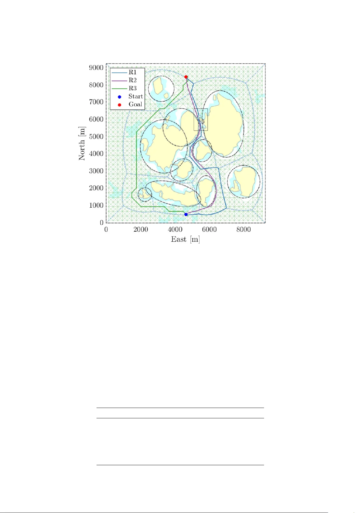
Impro v emen ts to W arm-Started Optimized T ra jectory Planning for ASVs Glenn Bitar B , Anastasios M. Lekk as and Morten Breivik Abstract W e present impro vemen ts to a recently dev elop ed metho d for tra jectory planning for autonomous surface v ehicles (ASVs) in terms of run time. The original metho d com bines tw o t yp es of planners: An A ? implemen tation that quickly finds the global shortest piecewise linear path on a uniformly discretized map, and an optimal con trol-based tra jectory planner which tak es into accoun t ASV dynamics. Firstly , we prop ose an improv ement to the discretization of the map by switching to a V oronoi diagram rather than the uniform discretization, which offers a far more sparse searc h tree for the A ? implemen tation. Secondly , mo difications to the path refinemen t are made, as suggested in a pap er by Bhattachary a and Gavrilo v a. The c hanges result in a reduction to the run time of the first part of the method of 85 % for an example scenario while maintaining the same level of optimalit y . 1 In tro duction Dev elopment of technology for autonomous surface vehicles (ASVs) is con tinuing at a rapid pace, moti- v ated by factors such as econom y , safety and the environmen t. In addition to academic interest, com- mercial organizations are diving in to the use of autonomous tec hnology . Among other use cases ASVs ha ve b een instrumen tal to reducing costs for o cean floor mapping surv eys, for instance in Alask a in 2016 (Orthmann, 2016). A t the base of any autonomous ship operation is a motion planning and control system. This type of system is resp onsible for planning and executing safe motion tra jectories that a void collision, and that promote some ob jectiv e, such as minimum time or energy consumption. Sev eral types of motion planners hav e been researched and dev elop ed for marine applications. In Figure 1 w e ha ve classified some t yp es of motion planning metho ds in to r o admap metho ds and optimal c ontr ol-b ase d metho ds . Roadmap methods build a path in the free space by exploring discrete points on the map. F urther, the roadmap metho ds can b e divided in to combinatorial metho ds that discretize all of the free space, and sampling-based metho ds that randomly explore p oin ts on the map. Optimal con trol-based metho ds build up on optimization, and are divided in to analytical methods that usually can only find solutions for very simple scenarios, and approximate metho ds which are more practical in real-w orld scenarios. A more in-depth background on these motion planning classes is provided in (Bitar et al., 2019). A com binatorial roadmap approach that is commonly used in path planning algorithms is the V oronoi diagram (Aurenhammer, 1991). The V oronoi diagram splits the workspace in cells according to gener- ator p oints, and is used in e.g. aerial (Bortoff, 2000) and marine (Candeloro et al., 2017; Gold, 2016) applications. Gold (2016) shows ho w V oronoi diagrams ma y b e used to build and dynamically up date 2D and 3D structures in geographic information systems. Bortoff (2000) prop oses a metho d where the path generated from the V oronoi diagram is used as an initial condition for a set of differential equations whic h at steady state optimize a fligh t path for a combination of distance to enem y radars and path length. The V oronoi diagram is also used as part of a more complex path planning scheme by Candeloro et al. (2017). Here the V oronoi diagram provides an initial path, which is subsequently refined, and then smo othed using F ermat’s spiral segmen ts. Despite the practical nature of such solutions, they cannot guaran tee that certain ob jectives, outside the shap e of the path itself, will b e satisfied. The authors are with the Cen tre for Autonomous Marine Op erations and Systems, and with the Department of En- gineering Cyb ernetics, Norw egian Univ ersity of Science and T echnology (NTNU), NO-7491 T rondheim, Norwa y . E-mails: { glenn.bitar,anastasios.lekk as } @n tnu.no, morten.breivik@ieee.org. The work is funded b y the Research Council of Norwa y and Innov ation Norwa y with pro ject number 269116. Additionally , the work is supp orted by the Centres of Excellence funding sc heme with pro ject num b er 223254. 1 Uniform decomp osition V oronoi diagram RR T PRM P ontry agin’s principle Dynamic programming Pseudosp ectral metho ds Multiple sho oting metho ds Com binatorial metho ds Sampling-based metho ds Analytical metho ds Appro ximate metho ds Roadmap metho ds Optimal control-based metho ds Pip elined optimization F ast, global Optimal, feasible Figure 1: Categorization of some motion planning algorithms. In (Bitar et al., 2019) w e hav e dev elop ed a pipelined tra jectory planning metho d that com bines adv antages from a roadmap metho d and optimal control. That metho d builds a tra jectory from a start p oin t to a goal p oint in a map of obstacles through three steps: Step 1: Discretize the obstacle map into a uniform grid, and p erform an A ? searc h to giv e the shortest path. Step 2: Refine path and add artificial temp oral information to conv ert it into a tra jectory . Step 3: Solve an optimal con trol problem (OCP) which gives an optimized tra jectory from start to goal, and warm start the solver with information from Step 2. This pap er presen ts improv ements to (Bitar et al., 2019) in terms of run time through the follo wing con tributions: • The uniform grid that discretizes the map in Step 1 of (Bitar et al., 2019) is replaced with a V oronoi diagram, which requires far fewer discrete nodes, increasing searc h sp eed. • The path refinement pro cess in Step 2 is improv ed with ideas from (Bhattachary a and Gavrilo v a, 2008). • The in tegration process in Step 2 that creates part of the initial guess for the OCP solv er is modified to increase sp eed. The improv ements cause a significant reduction in the run time of steps 1 and 2, while maintaining the same level of optimalit y . Preliminary topics are presented in Section 2. In Section 3 we briefly present the pip elined method from (Bitar et al., 2019), and describ e the improv ed metho d in more detail. Simulation scenarios and results are presented in Section 4, and we conclude the paper in Section 5. 2 Preliminaries In this pap er we utilize sev eral to ols that will b e briefly explained in this section. 2.1 V oronoi diagram A V oronoi diagram (Aurenhammer, 1991) partitions a plane in to regions based on distance to V or onoi gener ator p oints , or just generators for brevit y . These regions consist of all points closer to their generator than to any other generator. W e refer to those regions as V or onoi c el ls . A V oronoi diagram is useful in path planning since the edges of the V oronoi cells are distant to all obstacle in a map, if the generators lie along the obstacle b oundaries. The V oronoi cell edges are then candidates for paths in the map, and connect V or onoi vertic es in a searc hable graph. 2 A distinct adv antage of using V oronoi diagrams in path planning is that the graph can contain all p ossible paths b et ween obstacles, while the map is sparsely discretized (i.e. with a low n umber of V oronoi v ertices). An inherent disadv antage is that the V oronoi edges will b e placed far a wa y from the obstacle b oundaries, which increases path lengths. This disadv antage is addressed by using contributions from (Bhattac harya and Ga vrilov a, 2008). 2.2 A ? searc h T o be able to find an optimal (e.g. shortest) path in a map with the help of a V oronoi diagram, it is necessary to search the graph generated b y the V oronoi diagram in some w ay . In this paper we use A ? to search for the shortest path (Hart et al., 1968). A ? is a graph search algorithm guided b y a heuristic whic h quickly leads the search to the desired no de. 2.3 ASV mo deling W e use a mo del-based approach when generating our optimized tra jectory . The ASV is modeled mathe- matically by a set of differential equations which w e will present here. The equations are retrieved from (Bitar et al., 2019). A simple nonlinear 3-degree-of-freedom ship mo del is used, and the mo del has the form ˙ η = R ( ψ ) ν , (1a) M ˙ ν + C ( ν ) ν + D ( ν ) ν = τ ( u ) . (1b) The p ose vector η = [ x, y , ψ ] > ∈ R 2 × S contains the ASV’s p osition and heading angle in the Earth-fixed North-East-Do wn (NED) frame. The velocity vector ν = [ u, v , r ] > ∈ R 3 con tains the ASV’s bo dy-fixed v elo cities: surge, swa y and ya w rate, resp ectively . The rotation matrix R ( ψ ) transforms the b ody-fixed v elo cities to NED: R ( ψ ) =   cos ψ − sin ψ 0 sin ψ cos ψ 0 0 0 1   . (2) The matrix M ∈ R 3 × 3 represen ts system inertia, C ( ν ) ∈ R 3 × 3 Coriolis and centripetal effects, and D ( ν ) ∈ R 3 × 3 represen ts damping effects. The ASV is controlled b y the control vector u = [ X , N ] > ∈ R 2 , whic h con tains surge force and ya w moment. The control v ector is mapp ed to a force vector τ ( u ) = [ X, 0 , N ] > . 2.4 Optimal con trol problem T o find an optimized tra jectory , we solve an OCP , which is the challenge of finding a control and state tra jectory that minimizes an ob jective functional, while satisfying b oth differential and algebraic con- strain ts. In our case, w e p ose the tra jectory planning problem as an OCP in the following form, retrieved from (Bitar et al., 2019): min η ( · ) , ν ( · ) , u ( · ) Z t max 0 F ( η ( t ) , ν ( t ) , u ( t )) d t (3a) sub ject to ˙ η = R ( ψ ) ν ∀ t ∈ [0 , t max ] , (3b) M ˙ ν + C ( ν ) ν + D ( ν ) ν = τ ( u ) ∀ t ∈ [0 , t max ] , (3c) h ( η ( t ) , ν ( t ) , u ( t )) ≤ 0 ∀ t ∈ [0 , t max ] , (3d) e ( η (0) , ν (0) , η ( t max ) , ν ( t max )) = 0 . (3e) The solution of the OCP giv es state and input tra jectories that optimize the cost functional (3a), consisting of the cost-to-go function F ( η , ν , u ) = K e F e ( ν , u ) + K t F t ( ν ) , (4) with tuning parameters K e , K t > 0. The first term p enalizes energy usage and describes w ork done b y the actuators, while the second term is a disprop ortionate p enalization on turn-rate r , and prefers readily 3 Shortest piecewise linear path T ra jectory (initial guess) Energy- optimized tra jectory Scenario Ship mo del Step 1 Step 2 Step 3 A ? T ra jectory generation Optimal control Figure 2: Pip elined concept. observ able turns p erformed with high turn-rate. The idea for the turn-rate penalization is obtained from (Eriksen and Breivik, 2017). The same cost-to-go function is used in (Bitar et al., 2019). The solution will satisfy the dynamic constraints (3b) and (3c), as w ell as the inequality constrain t (3d) which enco des obstacles and state constraints, and (3e), which are the start and goal conditions. 2.5 T ranscription and solv er In order to solve the OCP from Section 2.4, it is transcrib ed to a nonlinear program (NLP) b y using a m ultiple sho oting approach. The transcription gives the follo wing NLP: min w φ ( w ) (5a) sub ject to g lb ≤ g ( w ) ≤ g ub , (5b) w lb ≤ w ≤ w ub . (5c) The details of the NLP structure are found in (Bitar et al., 2019). The NLP (5) is non-con vex, and a goo d solution is hard to find without a “goo d” initial guess. Solv ers generally find a lo cal optimum, and pro viding the solver with an initial guess is referred to as w arm-starting the solver. T o solve the NLP we use Casadi (Andersson et al., 2018) for Matlab, with the Ip opt solv er (W¨ ac hter and Biegler, 2005). 3 T ra jectory planning metho d with impro v emen ts In (Bitar et al., 2019) w e hav e dev elop ed a pipelined three-step metho d to obtain a dynamically feasible and optimized tra jectory b etw een a start and goal p osition in a map. Figure 2 shows ho w the pip elined concept w orks. In this pap er, impro vemen ts are made to the first tw o steps in terms of run time, and a comparative table of the steps in the metho d is pro vided in T able 1. The uniform grid discretization of Step 1 in (Bitar et al., 2019) is adv antageous in the sense that an arbitrary level of precision can b e obtained b y reducing the grid size ∆ d . Ho wev er, this leads to a large and dense search space, which results in a long run time of the A ? algorithm. As describ ed in Section 2.1, a V oronoi discretization of the map gives a sparse search tree, while still containing all p ossible routes. F or this reason, we switch to the V oronoi discretization. The V oronoi generators are p oin ts along the b oundary of each obstacle, as w ell as along the map edge. They are spaced with a distance of ∆ d , which is replacing the meaning of ∆ d in (Bitar et al., 2019). The disadv an tage of using a V oronoi discretization is also describ ed in Section 2.1; it leads to longer paths, since the V oronoi cell edges are inherently placed distan t from eac h obstacle. This motiv ates the adding of a path refinemen t pro cess to Step 2 of the method in order to shorten the path. The path refinemen t pro cess is the one developed by Bhattac harya and Ga vrilov a (2008), and consists of iteratively cutting corners of tw o edges b y trying to make collision-free connections b et ween intermediate points on the edges. W e also replace the w a yp oin t reduction process from (Bitar et al., 2019) with the more efficien t one describ ed in (Bhattac harya and Ga vrilov a, 2008). An additional improv ement to the run time of Step 2 from (Bitar et al., 2019) is achiev ed by c hanging the in tegration process for obtaining the w arm-started guess of the cost functional (3a). Instead of p erforming Runge-Kutta 4 integration of (4), we use the improv ed Euler method, removing the need for in terp olation of the warm-starting state and input tra jectories. 4 T able 1: Pip elined tra jectory planning metho d steps. Step Original metho d (Bitar et al., 2019) Impro ved method Qualitativ e changes 1 Discretize map into a uniform grid with cell sizes ∆ d × ∆ d . Search from start to goal with A ? . Discretize map into a V oronoi diagram using generators with spacing ∆ d on obstacle b oundaries. Searc h from start to goal with A ? . Impro vemen t results in a far more sparse search tree that still contains paths b et ween all obstacles, resulting in a faster A ? searc h. 2 P erform wa yp oin t reduction with a custom algorithm. Connect the path with circle arcs, and add artificial temp oral information. Use Runge-Kutta 4 integration for cost-to-go propagation. P erform wa yp oin t reduction and path refinement using algorithms from (Bhattachary a and Gavrilo v a, 2008). Connect the path with circle arcs, and add artificial temp oral information. Use improv ed Euler for cost-to-go propagation. Impro vemen t results in a go od and close-to-feasible initial guess for Step 3. The impro ved Euler propagation is muc h faster than Runge-Kutta 4, since there is no need for interpolation. 3 Solv e NLP (5) to retrieve a solution of the OCP (3), with the tra jectory from Step 2 as an initial guess for warm starting. Same as in (Bitar et al., 2019). No changes. 4 Sim ulation scenarios and results W e test the improv ed method on the example scenario presented in (Bitar et al., 2019), a small island group north of Sta v anger in Norw a y . First, w e presen t the difference in the discretization in Step 1 of the t wo results. T o demonstrate the adv an tage of using a V oronoi diagram discretization, w e also include a v ersion of the original method (Bitar et al., 2019) where the uniform grid size ∆ d is significantly increased. That results in a discretization that contains the same num b er of no des as the V oronoi diagram discretization in our example. F or conv enient referencing, w e enumerate the three differen t results as: R1: The improv ed metho d with V oronoi discretization. V oronoi generator spacing of ∆ d = 100 m. The discretized grid contains 833 non-colliding nodes. R2: The original metho d with dense discretization, as used in (Bitar et al., 2019). Grid size of ∆ d = 50 m. The discretized grid contains 22929 non-colliding no des. R3: The original method with sparse discretization. Grid size of ∆ d = 270 m. The discretize d grid con tains 843 non-colliding no des. Figures 3 and 4 sho w the discretized grids of the three results. W e see that the V oronoi diagram prop oses all p ossible routes b etw een the obstacles as paths. The dense grid from R2 also has all possible routes included in the searc h space, and the shortest piecewise linear path from those t wo grids go through the narro w passage in the cen tral part of the map. R3 has a muc h sparser discretization than R2, whic h causes the grid to be disconnected in the central narrow passage, leaving it out of the search space. This causes the searc h to find a differen t route in R3 than the routes from R1 and R2, to the left in the map. Figure 5 shows the tra jectories from the three results, along with their warm-start guesses. W e hav e used the same parameters as in (Bitar et al., 2019). Since the shortest piecewise linear paths from Step 1 in b oth R1 and R2 go through the central narrow passage, the OCP from Step 3 finds similar lo cally optimal tra jectories. On the other hand, Step 1 in R3 finds a path to the left in the map, causing a longer tra jectory . T able 2 sho ws how R1 and R2 give virtually equal energy consumption, but with a large reduction in run times for steps 1 and 2 in R1. The reduction in run time of Step 1 from R2 to R1 is attributed to the large reduction of nodes, simplifying the A ? searc h. The reduction in run time of Step 2 in the same comparison is attributed to the impro ved w a yp oin t reduction metho d, and the c hange of in tegration metho d, as detailed in Section 3. Comparing the run times of Step 1 in R1 and R3, w e see that it is 5 Figure 3: Grids and shortest piecewise linear paths from Step 1 of R1 and R3. The grid from R2 is not sho wn due to its high density , but is shown in a zo omed-in area in Figure 4. faster in R3. This may b e attributed to the increased complexity in p erforming the discretization with a V oronoi diagram, compared to the uniform grid. F or Step 3, the Ip opt solver uses more steps for R1 than R2, but also shorter time. These v ariations are due to the difference in initial guess. Ho wev er, we cannot say that this is a consistent effect from using the mo dified algorithms in steps 1 and 2, but state that they are arbitrary effects. Figure 6 shows the state tra jectories for the three results. It is w orth noting the higher a v erage surge v elo city u in R3 compared to the other tw o results. This is of course due to the increased length of the tra jectory , with the same amoun t of time to complete it. 5 Conclusion W e ha ve presen ted impro vemen ts in the pip elined tra jectory planning algorithm developed in (Bitar et al., 2019). The first improv emen t is to Step 1 of the algorithm, namely the discretization of the map in T able 2: Results. R1 R2 R3 Energy cost 2 . 75 · 10 7 [J] 2 . 74 · 10 7 [J] 3 . 85 · 10 7 [J] Run time 17 . 4 [s] 26 . 7 [s] 18 . 5 [s] Step 1 0.7 [s] 3 . 4 [s] 0.3 [s] Step 2 0.1 [s] 2 . 2 [s] 2 . 3 [s] Step 3 16 . 6 [s] 21 . 1 [s] 15 . 9 [s] Step 3 iterations 72 58 43 6 Figure 4: A zo omed-in version of Figure 3 with the grids from R1, R2 and R3. whic h to search for a global shortest path to goal. The uniform grid used in (Bitar et al., 2019) is c hanged to one based on V oronoi diagrams, which results in a sparse discretization of the search space that still con tains paths b et ween all obstacles. Run time for Step 1 is reduced from 3 . 4 s to 0 . 7 s in an example scenario. Because of the longer paths resulting from the use of V oronoi diagrams, a path refinement pro cess is added to Step 2, which shortens the path. Changes to the wa yp oin t reduction algorithm, and to the integration scheme used for finding an initial guess for the cost functional in Step 2, result in a reduction in Step 2 run time from 2 . 2 s to 0 . 1 s. T ogether this results in a reduction of 85 % in run time for steps 1 and 2 in the comparison scenario. As with the original method from (Bitar et al., 2019), the metho d is complete in terms of the shortest path, since this is the ob jective of the global A ? searc h. The V oronoi diagram k eeps paths b et ween all obstacles in the search space even when they are coarsely discretized. The implemented OCP provides lo cal optimality in the sense of a given ob jective function. Alone, the OCP solver will not find a global optim um, but guided by the initial guess, the OCP solver finds a lo cal minimum whic h may be close to the global optimum, dep ending on the ob jective function. The OCP will also return a feasible tra jectory , as the ASV dynamics are taken in to account. 7 Figure 5: Map and resulting tra jectories for R1, R2 and R3. W arm-starting tra jectories from Step 2 are sho wn in dashed lines. Figure 6: Heading, surge and sw ay v elo cit y and ya w rate tra jectories for R1, R2 and R3. 8 References Andersson, J. A. E., J. Gillis, G. Horn, J. B. Rawlings, and M. Diehl (2018). “CasADi – A softw are framew ork for nonlinear optimization and optimal control”. In: Mathematic al Pr o gr amming Compu- tation . Aurenhammer, F. (1991). “V oronoi Diagrams – A Survey of a F undamen tal Geometric Data Structure”. In: ACM Computing Surveys 23.3, pp. 345–405. Bhattac harya, P . and M. Gavrilo v a (2008). “Roadmap-Based P ath Planning - Using the V oronoi Diagram for a Clearance-Based Shortest Path”. In: IEEE R ob otics & Automation Magazine 15.2, pp. 58–66. Bitar, G., V. N. V estad, A. M. Lekk as, and M. Breivik (2019). Warm-Starte d Optimize d T r aje ctory Plan- ning for ASVs . Accepted to the 12th IF AC Conference on Con trol Applications in Marine Systems, Rob otics, and V ehicles. arXiv: 1907.02696 [eess.SY] . Bortoff, S. A. (2000). “Path planning for UA Vs”. In: Pr o c e e dings of the ’00 Americ an Contr ol Confer enc e . Chicago, IL, USA: IEEE, pp. 364–368. Candeloro, M., A. M. Lekk as, and A. J. Sørensen (2017). “A V oronoi-diagram-based dynamic path- planning system for underactuated marine vessels”. In: Contr ol Engine ering Pr actic e 61, pp. 41–54. Eriksen, B.-O. H. and M. Breivik (2017). “MPC-based Mid-lev el Collision Avoidance for ASVs using Nonlinear Programming”. In: Pr o c e e dings of the 2017 IEEE Confer enc e on Contr ol T e chnolo gy and Applic ations (CCT A) . Mauna Lani, HI, USA, pp. 766–772. Gold, C. (2016). “T essellations in GIS: Part II–making changes”. In: Ge o-sp atial Information Scienc e 19.2, pp. 157–167. Hart, P ., N. Nilsson, and B. Raphael (1968). “A formal basis for the heuristic determination of minimum cost paths”. In: IEEE T r ansactions on Systems Scienc e and Cyb ernetics 4.2, pp. 100–107. Orthmann, A. (2016). “Bering Sea ASV F orce Multiplier”. In: Hydr o International . url : https://www . hydro - international . com / content / article / bering - sea - asv - force - multiplier (visited on 2019-08-16). W¨ ac h ter, A. and L. T. Biegler (2005). “On the implemen tation of an in terior-p oin t filter line-searc h algorithm for large-scale nonlinear programming”. In: Mathematic al Pr o gr amming 106, pp. 25–57. 9