Joint Blind Identification of the Number of Transmit Antennas and MIMO Schemes Using Gerschgorin Radii and FNN
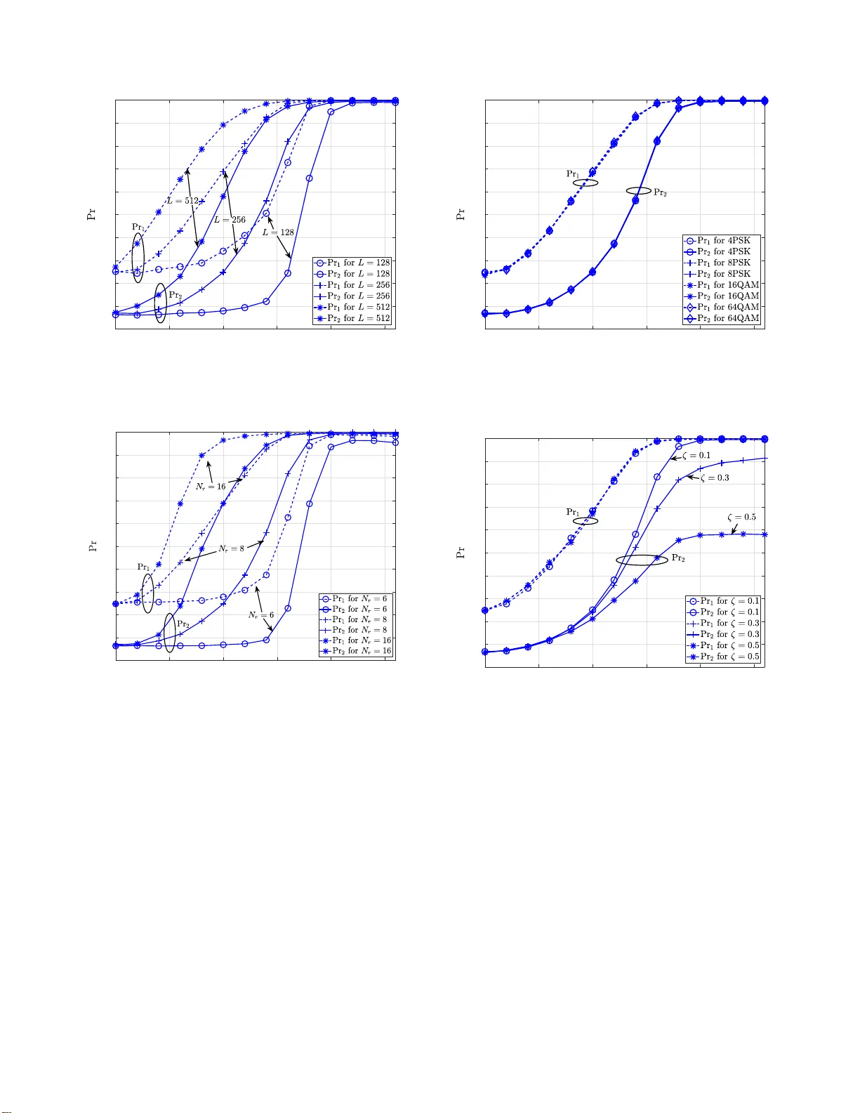
Blind enumeration of the number of transmit antennas and blind identification of multiple-input multiple-output (MIMO) schemes are two pivotal steps in MIMO signal identification for both military and commercial applications. Conventional approaches …
Authors: Mingjun Gao, Yongzhao Li, Octavia A. Dobre
1 Joint Blind Identification of the Number o f T ransmit Antennas and MIMO Schemes Using Gerschgorin Radii and FNN Mingjun Gao, Student Membe r , IEEE, Y ongzhao Li, Senior Memb er , IEEE, Octavia A. Dob re, S enior Me mber , IEEE, and Na ofal Al-Dhah ir , F ellow , IEEE Abstract —Blind enumeration of the number of transmit an- tennas and blind identifi cation o f multiple-inp ut multiple-outp u t (MIMO) schemes are two pivota l steps in MIMO signal ident i fica- tion f or b oth military and commer cial app lications. Con v entional approaches treat them as two i ndependent problems, namely the source number enu meration and the presence detection of space-time redund ancy , respectively . In this paper , we develop a joint blin d identi fication algorithm to determine the number of transmit antennas and MIMO scheme simultaneously . By restructuring the recei ved signals, we deriv e t hree subspace- rank features based on the signal subspace-rank to determine the number of transmit antennas and identify space-time re- dundancy . Th en, a Gerschgorin radii-based method and a feed- fo rward n eural network are employed to calculate these three features, and a minimal weighted norm-1 distance metric is utilized f or decision making . In particular , our approach can identify additional MIMO schemes, which most prev ious works hav e not considered, and is compatible with both sin gle-carrier and orthogonal frequency division multip lexing (OFDM) systems. Simulation results verify the viability of our p roposed approach fo r single-carrier and OFDM systems and demonstrate its fav or - able identification performance for a short observation period with acce ptable complexity . Index T erms —Joint b lind id entification, nu mber of transmit antennas, space-time b lock codes, orthogonal frequency division multiplexing, feed-f orward neural netwo rk (FNN). I . I N T R O D U C T I O N B LIND identification of info rmation signals’ parameter s of a tran smitter f rom r eceiv ed signals h as important applications both in m ilitar y an d c ivilian communica tion sys- tems. In the context o f militar y ap plications, th is p arametric knowledge can help an attacker to carry out electron ic warfare operation s, suc h as surveillance and jamming sign al selection. Moreover , blind ide ntification has fou nd wide applications in civilian r econfigur able systems inclu d ing software-defined and cognitive radios [1] . Multiple-in put mu ltip le-output (MIMO) and orth ogonal frequen cy d i vision multiplexing (OFDM) tech- nologies are adopted in cellular and WiFi standard s because they achieve h igh spectral ef ficien cy . Different fro m the iden- tification of single-an tenna systems, the b lind iden tification of MIMO or MIMO-OFDM signals requires the enu m eration o f the nu mber of transmit antennas [2]– [ 6] and identification o f MIMO schemes [7]–[2 3] f o r single- carrier or OFDM systems. The identificatio n of MIMO sch emes is the pro cess o f classifying th e spatial mu ltip lexing (SM) or tr ansmit diversity (TD) codes, namely space-time block codes (STBC), which utilize space - time redun dancy to reduce the error rate. Previous works on the identification of MIMO schemes in clude [7]–[1 6] for sing le-carrier systems a n d [17]– [23] for OFDM systems. Regarding the id entification of MIMO sch emes for single- carrier systems, previous works fo llow either likeliho o d-based [7] or feature- based [8]–[16] me th ods. The former relies on the likelihood f unction o f the r eceiv ed signa ls to quan tify the space-time red undancy and classify dif ferent STBCs. The latter detects the presence of the sp a c e-time redund ancy at some spe c ific time-lag locations based on the featur es of signal statistics or cyclic statistics; howe ver, it can on ly identify a small numb er of STBC typ es due to identical featu res for se veral SFBCs. Althoug h [1 6] can id entify 11 types of STBCs utilizing the fea ture of seco nd-ord er cyclostationary statistics, it req uires the numb er of transmit anten nas and channel coefficients as a priori inform ation. As for OFDM systems, there are two m ain app r oaches to combine the TD codes with OFDM signals. Th e first appr o ach is STBC-OFDM, where the diversity STBC is implemen ted over c onsecutive OFDM symbol intervals. STBC-OFDM has been adopted in several in d oor MIM O wireless standar ds, such as WiFi [24], [25], owing to its excellent p erforman ce. Anoth er TD coding scheme used in OFDM system s is spac e-freque n cy block codin g (SFBC)-OFDM, where th e diversity SFBC is employed over consecutive subca rriers of a n OFDM symbo l. Sev e r al cellular wireless stand ards suppo rting h ig h mobility , such a s L TE [26] and W iMAX [27], fav or SFBC-OFDM over STBC-OFDM bec a use of its superior perfo rmance in a high mob ility en v ironmen t [28]. The id entification appr oaches for single-carr ier systems fail to id entify MI MO schemes of OFDM systems under freq uency-selective fading chann e ls due to mu ltipath effects. Previous work s on th e identification of STBC-OFDM systems include [ 17]–[19], which detect the presence of spa c e-time redundancy b ased o n th e peaks of the cross-corre lation func tions betwe e n two recei ve antennas in the time -domain. Specifically , [1 7], [18] u se different cro ss- correlation function s, while [19] employs a cyclic cro ss- correlation fu nction with a specific time-lag durin g ad jacent OFDM symb ols to detect the sp a c e-time redu n dancy . Howe ver, the ap proaches f or id e ntifying STBC-OFDM signals cannot be dire ctly applied to SFBC-OFDM signals since the pe a ks of the cross-co r relation fun ctions b etween two adjacent OFDM symbols are difficult to detect. The pr evious w o rks on the identification of SFBC-OFDM systems in clude [2 0]–[23]. In [20], the id ea of d etecting the p eak o f the cross-correlation function between two r eceiv e an tennas is extend e d to id entify 2 SFBC-OFDM signals, whic h u ses a specific time-lag du ring the same OFDM symbo l. In [21], [22], we utilize a cross- correlation f unction betwee n two receive ante n nas at adjacent OFDM subcarr iers to improve the iden tificatio n per f ormance by d etecting bo th the space and frequency redun dancy . In [23], we use the random matrix theo ry to identify 5 types of SFBCs b y detectin g the space- f requency r edundan cy at adjacent OFDM subcarriers. Ho wever , most pre v ious works can only discriminate betwe e n a few MIMO schem e s since they only co nsider d etecting th e p r esence of th e re dundan cy . Specifically , a widely-used TD code, namely the frequency switched tr a nsmit diversity ( FSTD) [26], [27], and sev e r al non- orthog onal ST BCs/SFBCs can no t b e discrimin ated by the pre- vious n on-likelihood -based methods. Althoug h the likelihood- based method [7] can ide n tify more STBCs, it doe s not work in a freque n cy-selecti ve fading en viro nment. In the existing literature, th e enumeration of the number of transmit anten nas and identification of MIMO schemes are hand led as two ind e pendent pro blems. T he en umeration problem of th e num ber of transmit antenn as is formula te d as the enum e r ation of indepen dent channel pathways between transmit a n tennas and receiv e antennas in genera l. Pr e vious works on the identification o f the numbe r of tran smit an- tennas mainly fall into two classes, namely second- [ 2]– [5] and higher-order statistics-based meth ods [6]. Basically , the second-o rder statistics-based method s analyze eigenvalues or eigenv ectors of the covariance matrix of the received signals to determine th e n u mber of tran smit antenn as by disting u ishing between the signal and noise subspaces. These method s also fall under two categories, information -theoretic criter ia - based algorithm s [2] and hypo thesis-testing-based algorithms [3]– [5]. Methods in the first category determin e the number of transmit an tennas b y minimizing the Kullback-Leibler distan ce metric. Referen c e [2] introduces two classical calcu lations of the Kullback-Leibler metric, th e Akaike in f ormation criterion (AIC) and the minimum description len gth (MDL), for the enumera tio n of the number of transmit anten nas. Methods in the second category tra n sform the problem in to a detection problem , which compares an elab orately constru cted statis- tic with a th reshold. Fur thermore, for the class o f hig h er- order statist ics-based methods, the sole existing algo rithm [6] constructs a fo u rth-ord er de c ision statistic of the rec e i ved signals with only one receiv e a ntenna by using the feature of time-varying block fading cha nnels. T o the best of our knowledge, no meth od exists in the literature f or the joint blind identification of the number of transmit antennas and MIMO schemes. It is our main go al in this paper to fill this research gap. Artificial neural n etworks (ANN) h ave been applied to signal identification pr o blems, such a s autom atic modu lation classification (AM C) [29]–[32], since they ar e suitable fo r non- linear fitting an d classification problems an d do no t impo se any restrictions on the input variables, un like other p rediction technique s. Traditional ANNs require e xpert featu res, while modern deep learn ing neu r al networks ca n directly learn the statistical featu res fro m training data. References [31], [32] use deep lea r ning neural network s on the r aw in- phase and quadr ature ph ase (IQ) data to solve the AMC prob lem. Howe ver, their goal is to classify the single-an te n na system. For the MIMO system, it is difficult to dir ectly emp loy deep learning o n th e r aw IQ data since MIMO overlapped signals destroy the statistical featur es. Giv e n that the feed-f orward neural network (FNN) is a popular family of ANN o wing to its simple structu re and stro ng fitting ability , it is used to develop high performan ce signal identification solution s [ 29], [30]. As mentioned earlier , the quantification of the space- time/frequ e ncy redun dancy can classify more STBCs/SFBC s since th e redu n dancy of some STBCs/SFBCs is in the same location. On th e oth er h and, this quantification is also n eeded in the enumer ation of the nu mber of tran smit antenn a s. In this paper, a subspace- r ank fea ture-based join t blind iden tification algorithm of the numb e r of transmit antennas and MIMO schemes is p roposed. Th r ee different subspace- rank feature s for the number of transmit an tennas an d re dundan cy ar e derived from th e eige n value analysis of the cov arian c e matrix of th e received sign als at adjacen t symb ols or OFDM sym- bols/subcarr iers w ith mu ltiple recei ve antenn as. A Gerschg orin radii-based metho d and an FNN are app lied to ca lc u late th ese features, an d a m inimal weighted norm -1 distance metric is propo sed to deter mine the n umber o f transmit antenn a s a n d MIMO schem es. The p roposed algor ith m d oes not require a priori kn owledge of the sign al param eters, such as chann el coefficients, mod ulation type or noise p ower . The main contributions o f this paper a r e the following: • The prop osed algorith m jointly ide ntifies the numb er of transmit anten nas and MIMO sch emes, which has no t been considered in the previous works. • The scenarios of sing le-carrier a nd OFDM, inclu d ing STBC-OFDM and SFBC-OFDM ar e all investigated in this paper, unlike previous works. • Unlike the existing algorithms, more STBC/SFBC types, such as th e ortho gonal STBCs/SFBC s (OSBC) with the same rate, FSTD, qu asi-orthog onal STBC/SFBC (QOSBC) and no n -ortho g onal STBCs/SFBCs (SBC), ar e identified by the p roposed alg orithm thanks to the a nal- ysis of subspace-rank features. • A Gerschg o rin r adii-based method and an FNN are efficiently combined to calculate the subspace-ran k fea- tures. Fu r thermore , we extend the investigation to OFDM systems. • The co mputationa l co mplexity of th e prop osed algorith m is analyzed and shown to be co m parable to the enu mera- tion algorithm of th e number o f tran smit antennas in [2] or identification algorithm of MIMO schemes in [7]. • Simulation results are presented to demon strate the v ia- bility of the p roposed algorithm both in single- carrier and OFDM systems, with different system par a meters. This pa per is organized as follows. In Section I I , the system model is introdu ced. Then , Sectio n III der i ves the th ree subspace-ra n k features. The propo sed algor ith m is describe d in Section IV . Th e simulations resu lts are pr esented in Section V . Finally , conclusion s are drawn in Section VI. Notatio n: The following nota tio n is used throughou t th e paper . Th e superscripts ( · ) ∗ , ( · ) T and ( · ) H denote the complex conjuga te , tran sposition and conjugate tr ansposition, respec- ti vely . P r ( B ) r e p resents the prob ability of the event B . E [ · ] 3 Fig. 1. System s tructures and signal mappings of STBC/SFBC. indicates the statistical expectatio n. ℜ {·} and ℑ {·} den ote the real and imag inary parts, respectiv ely . I , 0 and O d e n ote the identity matrix , ze ro vector and zero matrix, re sp ecti vely . N , Z + and C are the set of natural numbe r s, positiv e integers and complex num b ers, resp e cti vely . The notation ca r d( A ) den o tes the cardina lity of th e set A . T r( · ) denote s the trace o f a matrix. Con ventionally , e an d log denote th e Euler con stant and natural logarithm , r espectiv ely . Fin ally , O ( · ) deno tes the complexity order . I I . S Y S T E M M O D E L A. S ignal Model of MIMO Single-Carrier System W e co nsider a M I MO single-carr ier wireless commu nication system employing TD or SM with N t transmit antenn a s and N r ( N r > N t ) recei ve a n tennas, as shown in Fig. 1 (a). As a special case, single-ante n na systems a re also considered . Th e transmitted data symbo ls are drawn from an M -PSK (Phase- Shift-Keying) or M -QAM (Quadratu re Amplitud e Modula- tion), M ≥ 4 , sign al co nstellation. Subsequen tly , th e modu - lated symbo l stream is p arsed into a data blo c k of N s symbols, denoted by the vector x b = [ x b, 0 , · · · , x b,N s − 1 ] T ( b ∈ N ) . A TD/SM encod er takes the row of an N t × T codeword matrix, denoted by C ( x b ) , to span T co nsecutive time slots and maps every co lumn of the ma trix into N t different transmit antennas. In this paper, the codewords include the single- antenna, Alamo uti (AL), SM , 7 types o f OSBC [33]–[ 35], one type of QOSBC [36], FSTD in L TE [ 2 6] and 3 typ es of SBC in W iMAX [27] (see Appendix A). T hen, mapped signa ls are tran sm itted after the p ulse shaping an d carr ier modulation operation s. The receiver is assumed to successfu lly synchron ize the received signals at th e b eginning to simplify the analysis; howe ver, later we analyz e the sen siti v ity to model mismatch es in Section V . W e co nstruct an N t × 1 tr a nsmit vector and an N r × 1 receive vector, denoted by s ( n ) a n d y ( n ) , which represent the transm itted and receiv ed signals at th e n -th ( n ∈ Z + ) time slot, respectively . The chan nel is assumed to be flat-fading and char acterized by an N r × N t matrix of Rayleigh fading coef ficients, denoted by H = h (1 , 1) · · · h ( N t , 1) . . . . . . . . . h (1 ,N r ) · · · h ( N t ,N r ) (1) where h ( f 1 ,f 2 ) represents the chann e l coefficient be twe en the f 1 -th tran smit antenn a an d f 2 -th rece i ve anten na. The channel matrix H is assumed to be of full-c olumn ran k an d the chan nel gains remain con stant over th e observation in terval. Then, th e 4 n -th received signal is described by the following mo del y ( n ) = Hs ( n ) + w ( n ) (2) where the vector w ( n ) represents a white Gaussian noise vector with zero- mean an d covariance σ 2 w I N r . T h e first pro - cessed sam p le is assumed to b e the start of a TD cod e blo ck, which allows simplification s of the following mathematical expressions. However , extension s of the pro p osed metho ds c a n be easily obtained when this assumption does not hold. B. S ignal Model of MIMO-OFDM S ystem 1) STBC-OFDM System: Consider a MIM O-OFDM wire- less comm u nication system with N sub carriers and a cyclic prefix (CP) o f length ν , as shown in Fig. 1 ( b ). Different from th e single-car r ier system, the TD/SM en coder p uts N data block s, de n oted b y x b , · · · , x b + N − 1 , on N con secutiv e subcarriers with the same oper ation as the single- carrier sys- tem. At the receiver side, assume tha t the car rier type is successfully estimated which can b e a c hiev ed based on th e cyclic cumu lant [37]. the received OFDM sym bol is converted into a frequ ency-domain block via an N -point fast Fourier transform (FFT) after removing the CP . W e constru ct an N t × 1 transmit vector and an N r × 1 receiv e vector , denoted by s k ( n ) , and y k ( n ) , which represen t the transmitted and received signals at the n -th time slot and k -th ( 1 ≤ k ≤ N ) subcarrier, respectively . The chann e l is assumed to be fr e q uency-selective fading an d the k -th sub c hannel is characte r ized by an N r × N t full-rank matrix of fading coefficients, denoted by H k . Then, the n -th r eceiv e d sign al at the k -th subcarrier is described by the following mod el y k ( n ) = H k s k ( n ) + w k ( n ) (3) where the N r × 1 vector w k ( n ) repre sents a freq u ency-doma in white Gaussian noise vector at the k - th subcarrier . 2) SFBC-OFDM System: The SFBC-OFDM system mo del is similar to the STBC-OFDM system model, with the differ- ence that th e SFBC encod er takes the row of the co dew ord matrix C ( x b ) to span T consecutiv e sub carriers d irectly ( T is the nu m ber of th e column of C ( x b ) ). The thr ee mappin gs are shown in Fig. 1 (c) . I I I . S U B S PAC E - R A N K F E A T U R E S O F D I FF E R E N T N U M B E R S O F T R A N S M I T A N T E N NA S A N D M I M O S C H E M E S In this section, three subspace -rank fea tures are defined as d iscriminating fe a tures of different MI MO scheme s, by considerin g the dimension of the subspa c e of restru c tured received sign als. Wi thout lo ss o f gener ality , we consider the single-carrier system first and th e n extend the analysis to the OFDM system. A. Numb er of T ransmit Antennas F eature Let us construct a time- domain recei ve window to observe the received sig n als at adjacent time slots. The wind ow leng th is set to two since it is the fin est gr a n ularity to q uantify the features of different MIMO schemes, while a larger window length results in failure to d istinguish many MIMO schemes. By u sing (2), the l -th rece i ved sign al b lo ck inside the window is expressed as Y ( l ) = HS ( l ) + W ( l ) (4) where the tr ansmitted signal block of adjacent time slots is denoted by an N t × 2 matrix S ( l ) = [ s ( l ) , s ( l + 1)] , a nd the noise vector is denoted by W ( l ) = [ w ( l ) , w ( l + 1)] . The covariance matrix of the received block is Σ Y ( l ) = E [ Y ( l ) Y H ( l )] = H Σ S ( l ) H H + 2 σ 2 w I N r (5) where Σ S ( l ) = E[ S ( l ) S H ( l )] is th e covariance matrix of the l -th transmitted block. De n oting the eigenv alues of Σ Y ( l ) by in descen ding order, we have the eigen values ϕ 1 ( l ) ≥ ϕ 2 ( l ) · · · ≥ ϕ N r ( l ) . Pr oposition 1: The smallest N r − N t ordered e igen values of Σ Y are all equal to 2 σ 2 w , i.e., ϕ N t +1 = · · · = ϕ N r = 2 σ 2 w if the rank of Σ S is N t . Pr oof: See Appen d ix B. The correspo n ding eigen vector s of the eigenv alu e s ϕ 1 ( l ) , ϕ 2 ( l ) · · · , ϕ N r − N t ( l ) form a b asis f or the signa l subspace. Define the following subset of signa l su bspace eigenv alues of Σ Y ( l ) A l = { ϕ 1 ( l ) , ϕ 2 ( l ) · · · , ϕ N r − N t ( l ) } . (6) By slidin g the window , the cardinality o f th e set A l with even subscript ( l = 2 m , m ∈ Z + ) can be u sed a s the first ty pe of the subsp ace-rank feature since the cardinality of A 2 m − 1 for FSTD is eq ual to two. Theref ore, we d efine this cardin a lity as the number of transmit-antenna feature (NT AF), deno ted b y α = card( A l ) , l = 2 m, m ∈ Z + . (7) Note that the NT AF , α , is th e discrimin a ting feature for different n umbers of transmit antennas. B. Numb er of Independen t Comp le x Symbols F eature Let us vector ize the l -th sig n al and no ise block inside the window in (4) as follows ¯ y ( l ) = y ( l ) y ( l + 1) , ¯ s ( l ) = s ( l ) s ( l + 1) ¯ w ( l ) = w ( l ) w ( l + 1 ) . (8) Then, the l - th r eceiv e d vector ized b lock is re written as ¯ y ( l ) = ¯ H ¯ s ( l ) + ¯ w ( l ) (9) where the 2 N r × 2 N t matrix ¯ H is ¯ H = H O O H . (10) Like (5), the covariance ma trix o f the l -th received vectorized block is Σ ¯ y ( l ) = E[ ¯ y ( l ) ¯ y H ( l )] = ¯ HΣ ¯ s ( l ) ¯ H H + σ 2 w I 2 N r (11) where Σ ¯ s ( l ) = E[ ¯ s ( l ) ¯ s H ( l )] is the covariance ma trix o f the l -th transmitted vectorized blo ck. The e ig en values of Σ ¯ y ( l ) are φ 1 ( l ) ≥ φ 2 ( l ) · · · ≥ φ 2 N r ( l ) . 5 Next, we define the no tion of linearly indepen dent ran- dom symbols. Let v 1 , · · · , v n be the vector observa- tions of the rand om variables v 1 , · · · , v n . T hen, we de- fine v 1 , · · · , v n as linearly indepen dent rando m symbols if the eq uation c 1 v 1 + c 2 v 2 + · · · + c n v n = 0 can only be satisfied by c i = 0 for i = 1 , · · · , n [38]. For example, assuming u = [ v 1 , v 2 , v 3 / √ 2 , − v ∗ 2 , v ∗ 1 , v 3 / √ 2] T whose eleme n ts are com plex random v ariables, then u has fiv e linearly indepen dent co mplex r andom sym- bols, i.e., v 1 , v 2 , v 3 / √ 2 , v ∗ 1 , − v ∗ 2 . Assumin g u = [ ℜ ( v 1 ) , ℑ ( v 1 ) , ℜ ( v 2 ) , ℑ ( v 2 ) , ℜ ( − v ∗ 2 ) , ℑ ( − v ∗ 2 ) , ℜ ( v ∗ 1 ) , ℑ ( v ∗ 1 )] T , then u has fo ur linearly ind ependent real random symbols, i.e., ℜ ( v 1 ) , ℑ ( v 1 ) , ℜ ( v 2 ) , ℑ ( v 2 ) . Pr oposition 2 : Assume that M c is the n u mber of line arly indepen d ent complex rando m sym bols o f a transmitted vec- torized b lock. T h e smallest 2 N r − M c ordered e ig en values of Σ ¯ y are all equal to σ 2 w , i.e., φ M c +1 = · · · = φ 2 N r = σ 2 w . Pr oof: See Appen d ix B. Similarly , let us define a su b set of the sign al subspace eigenv alues of Σ ¯ y as B l = { φ 1 ( l ) , φ 2 ( l ) · · · , φ M c ( l ) } . (12) By sliding the window , we can select the car dinalities of three sets, namely B l 1 , B l 2 and B l 3 with subscripts l 1 = 4 m − 3 , l 2 = 4 m − 2 , an d l 3 = 4 m − 1 ( m ∈ Z + ), respec tively , as the second typ e of subspace- r ank features to iden tify more MIMO schemes in the MIMO scheme p o ol. T hen, we define th ree linearly indepen dent c omplex ra n dom-sym bol f eatures (ICSF), which represent the cardinalities of the three sets, denoted by β 1 = card ( B l 1 ) , l 1 = 4 m − 3 , m ∈ Z + (13a) β 2 = card ( B l 2 ) , l 2 = 4 m − 2 , m ∈ Z + (13b) β 3 = card ( B l 3 ) , l 3 = 4 m − 1 , m ∈ Z + . (13c) C. Number of Independ ent Real Symbo ls F e atur e By stacking the r eal a nd imaginar y parts of the block inside the wind ow in (8), we ob tain a tran smitted, a rec e i ved stacked block and the noise block as ˜ y ( l ) = ℜ ( y ( l )) ℑ ( y ( l )) ℜ ( y ( l + 1)) ℑ ( y ( l + 1)) , ˜ s ( l ) = ℜ ( s ( l )) ℑ ( s ( l )) ℜ ( s ( l + 1)) ℑ ( s ( l + 1)) ˜ w ( l ) = ℜ ( w ( l )) ℑ ( w ( l )) ℜ ( w ( l + 1)) ℑ ( w ( l + 1)) . (14) Similarly , the l -th received stacked block is rewritten as ˜ y ( l ) = ( I 2 ⊗ ˜ H ) ˜ s ( l ) + ˜ w ( l ) (15) where the 2 N r × 2 N t matrix ˜ H is gi ven by ˜ H = ℜ ( H ) −ℑ ( H ) ℑ ( H ) ℜ ( H ) (16) and ⊗ corr esponds to the Krone c ker prod uct. Then , the covariance matrix of ˜ y ( l ) is Σ ˜ y ( l ) = E [ ˜ y ( l ) ˜ y T ( l )] = ( I 2 ⊗ ˜ H ) Σ ˜ s ( l )( I 2 ⊗ ˜ H T ) + σ 2 w 2 I 4 N r (17) where Σ ˜ s ( l ) = E [ ˜ s ( l ) ˜ s T ( l )] is the covariance matr ix of the l -th tran smitted stacked b lo ck. Th e eig en values o f Σ ˜ y ( l ) are η 1 ( l ) ≥ η 2 ( l ) · · · ≥ η 4 N r ( l ) . Pr oposition 3 : Assume that M r is the n u mber o f lin early indepen d ent real random symb ols o f a transmitted stacked block. The smallest 4 N r − M r ordered eigenv alue s of Σ ˜ y ( l ) are all equal to σ 2 w / 2 , i.e., η M r +1 = · · · = η 4 N r = σ 2 w / 2 . Pr oof: See Appen d ix B. Let us d efine th e fo llowing sub set o f the signal subspace eigenv alues of Σ ˜ s ( l ) as C l = { η 1 ( l ) , η 2 ( l ) , · · · , η M r ( l ) } . (18) By sliding the window , the card inalities of the sets C l 1 and C l 2 with subscripts l 1 = 4 m − 3 an d l 2 = 4 m − 1 ( m ∈ Z + ), respectively , are chosen to be the third ty pe of subspace-rank features since the cardinalities of the o th er sets ca n not be used to identif y several TD cod es with dif f erent tran smission rates. Then, we defin e two linearly indepen d ent real rand om-symb o l feature (IRSF) representing these cardinalities gi ven by γ 1 = card ( C l 1 ) , l 1 = 4 m − 3 , m ∈ Z + (19a) γ 2 = card ( C l 2 ) , l 2 = 4 m − 1 , m ∈ Z + . (19b) Actually , the I CSF and IRSF can qu antify the space-time redund ancy . For different MIMO scheme s with the same number o f tran smit antenn as, the transmitted signal b lock inside the wind ow has more spac e-time r edundan cies, or in other words, the blo ck transmits some identical symbols due to the structure of the codew o rd matrix . Therefore, smaller ICSFs and I RSFs values are calculated a t the r eceiv e r since these symbols are linearly dependent. All signal featur es using d ifferent n u mbers of transmit antennas an d com mon MIM O schemes are listed, and a representative exam ple ar e described in Appendix C. D. S ubspace-R ank F eatu r es in the OFDM System 1) STBC-OFDM Case: Since STBC-OFDM is a direct extension o f ST BC single-car rier , we can use the l -th re c ei ved signal b lock at the k - th subc arrier, d enoted by Y l ( n ) , to der i ve the NT AF , I CSFs and IRSFs as w e d escribed previously . 2) SFBC-OFDM Case: Regarding the SFBC-OFDM sy s- tem, we constru c t and slide a fr equency-do main re c ei ve w in - dow to ob ser ve the r eceiv ed signals at ad jacent subcarr iers an d calculate the sub space-rank fe atures. T hus, th e l -th received block, vectorized bloc k and stacked block in ( 4), (8) and (14) inside the window are, respectively , modified to Y l ( n ) = [ y l ( n ) , y l +1 ( n )] , ¯ y l ( n ) = y l ( n ) y l +1 ( n ) ˜ y l ( n ) = ℜ ( y l ( n )) . . . ℑ ( y l +1 ( n )) . (20) 6 I V . P RO P O S E D B L I N D I D E N T I FI C A T I O N A L G O R I T H M In this section, we use a Ger schgorin r adii-based m ethod and an FNN to calculate th e subspace-ra n k featu res and employ a minimal weighted n orm-1 distance metric to discrim- inate between these fea tu res. Different from the original Ger- schgorin radii- based method in [ 39], the r adii of th e circles are compressed after a similarity transforma tion, and then, an FNN is used to calculate the subspace-r ank fe atures. Additiona lly , extensions to the ST BC-OFDM and SFBC-OFDM systems are p r oposed by combinin g the calculations from different subcarriers after an analysis of the channel response. A. P r o posed Algorithm for Single-Carrier System The cov ariance matrices estimators ar e giv en b y ˆ Σ α = 1 L/ 2 − 1 L/ 2 − 1 X m =1 Y (2 m ) · Y H (2 m ) (21a) ˆ Σ β 1 = 1 L/ 4 L/ 4 X m =1 ¯ y ( 4 m − 3) · ¯ y H (4 m − 3) (21b) ˆ Σ β 2 = 1 L/ 4 L/ 4 X m =1 ¯ y ( 4 m − 2) · ¯ y H (4 m − 2) (21c) ˆ Σ β 3 = 1 L/ 4 L/ 4 X m =1 ¯ y ( 4 m − 1) · ¯ y H (4 m − 1) (21d) ˆ Σ γ 1 = 1 L/ 4 L/ 4 X m =1 ˜ y (4 m − 3) · ˜ y T (4 m − 3 ) (21e) ˆ Σ γ 2 = 1 L/ 4 L/ 4 X m =1 ˜ y (4 m − 1) · ˜ y T (4 m − 1 ) (21f) where L is th e numbe r o f symbols. For convenience, we employ a com m on notation, ˆ Σ , to represent the estimated covariance matrices in (21). Assume that ˆ Σ is a J × J matrix . First, we partition the estimated cov ar iance matrix as ˆ Σ = a 11 a 12 · · · a 1 J a 21 a 22 · · · a 2 J . . . . . . . . . . . . a J 1 a J 2 · · · a J J = Σ 1 a a H a J J (22) where the red u ced covariance matrix Σ 1 is a ( J − 1) × ( J − 1) leading p r incipal su b matrix of ˆ Σ obtained by removing the last row and co lumn o f ˆ Σ . Then, the reduced covariance m atrix Σ 1 can be decomp o sed by its eigen structure as fo llows Σ 1 = Q 1 Λ 1 Q H 1 (23) where Λ 1 is a d iagonal matrix constructed f rom the eigen val- ues of Σ 1 as Λ 1 = diag( µ 1 , µ 2 , · · · , µ J − 1 ) (24) and Q 1 is a ( J − 1) × ( J − 1) unitary matrix form ed by the correspo n ding eigenvectors as follows Q 1 = [ q 1 , q 2 , · · · , q J − 1 ] . (25) Then, we construct the following J × J unitary transfor mation matrix Q 2 = Q 1 0 0 T 1 (26) where Q 2 Q H 2 = I . The transformatio n of ˆ Σ is R = Q 2 ˆ ΣQ H 2 = Λ 1 Q H 1 a a H Q 1 a J J = µ 1 0 · · · 0 ρ 1 0 µ 2 · · · 0 ρ 2 . . . . . . . . . . . . . . . 0 0 · · · µ J − 1 ρ J − 1 ρ ∗ 1 ρ ∗ 2 · · · ρ ∗ J − 1 a J J (27) where ρ i = q H i a for i = 1 , 2 , · · · , J − 1 . Th us, the radius of the i -th Gerschgorin circle is r i = | ρ i | = | q H i a | . (28) In o rder to scale the rad ii of Gerschg orin circles in propo rtion, we construct the diagonal matrix P = dia g( µ 1 , µ 2 , · · · , µ J − 1 , µ J ) (29) where µ J is the mean of th e eigen values µ 1 , · · · , µ J − 1 giv en by µ J = 1 J − 1 J − 1 X i =1 µ i . (30) The matrix R can be similarly transformed into R ′ = PRP − 1 = µ 1 0 · · · 0 µ 1 µ J ρ 1 0 µ 2 · · · 0 µ 2 µ J ρ 2 . . . . . . . . . . . . . . . 0 0 · · · µ J − 1 µ J − 1 µ J ρ J − 1 µ J µ 1 ρ ∗ 1 µ L µ 2 ρ ∗ 2 · · · µ J µ J − 1 ρ ∗ J − 1 a J J . (31) Practically , the centers of the Gerschg orin circles are fixed while their r adii are relatively sque e zed by th e factor µ i /µ J . The Gerschgor in circles of the noise su b space ar e squee z ed more th an those of the sig n als since the noise circles radii are generally smaller than µ J . Then , the radii of the comp ressed Gerschgor in circles for i = 1 , · · · , J − 1 , ar e den o ted by R i = µ i ρ i µ J = µ i µ J r i . (32) After extracting the radii of the com pressed Gerschgorin circles, the iden tificatio n prob lem can b e considered as a fitting problem of the Gerschg orin circles which determine s h ow many Gerschgorin circ le s a re those of the signal subspace. Howe ver, the r a d ii of the Ger schgorin cir cles of th e signal and noise subspaces have a wide range un der different condition s, including signal-to-noise r atio (SNR), th e nu m ber of pro c e ssed samples a nd nu mber o f receive an tennas, which results in the non-lin e arity between the inp uts an d outpu ts of the lea r ning system. In this pap er , since an FNN can fit a ny finite inp ut-outpu t mapping problem a nd has a simple stru cture, we use a three- layer FNN, as shown in Fig. 2, to de te r mine the numbe r of 7 Ă Ă Ă Ă Ă Fig. 2. FNN for the calculati on of the Gerschgorin radii. the signal-sub space Gerschgor in circles. The FNN in cludes an input layer, a h idden la y er and an output layer . The h id den layer has 10- 2 0 neu rons using the sig moid tran sf e r fu nction while the o utput layer only has o n e linear neu r on. Af ter th e SNR is normalize d , the Levenberg-Marquard t b a c kpropa g ation algorithm [40] is utilized to train the FNN by using test data. T o av o id overfitting, we use a large set of data to train th e FNNs, which is descr ibed later o n in Section V . Then, the feature value is a fitting function o f the radii of co mpressed Gerschgor in circles given by Q = f ( R 1 , R 2 , · · · , R J − 1 ) . (33) The quantity Q represents the calculated feature, ˆ α , ˆ β 1 , ˆ β 2 , ˆ β 3 , ˆ γ 1 or ˆ γ 2 depend ing on the corr e sp onding covariance matrix in Eq uations (2 1a)-(21f). Since the sizes of the covariance matrices and the eigenv alues after d ecomposition have large differences for the three su bspace-ran k featu res, the nu mbers and values (the distributions of values of the radii) of the FNN inpu ts are significan tly different for different features. T o enhance p erform a n ce, we use th ree train e d FNNs to determ ine { ˆ α } , { ˆ β 1 , ˆ β 2 , ˆ β 3 } and { ˆ γ 1 , ˆ γ 2 } , respectively . Finally , since the MIMO scheme C contains the infor mation on the number of transmit antenn as N t , they are simultan eously determined by a minimal weighted norm-1 distance metric gi ven by ˆ N t , ˆ C = a rg min C ∈ { CODE } (24 · | ˆ α − α | + 4 · X i ˆ β i − β i + 3 · X i | ˆ γ i − γ i | ) (34) where th e notation {CODE} ref ers to the set of all scheme s listed in T ab le I V (see Append ix C). The reason for em ploying a no r m-1 distance metric is th at it is more r obust again st outliers than oth er distance metrics [4 1]. Th e weig hting co ef- ficients are cho sen to eliminate the bias ca used by the features with larger values and equal to th e least commo n multip le of the NT AF , sum of ICSFs and sum of I RSFs for single-anten n a, which is equal to 24, di vid ed b y these values resulting in the weighting coefficients of 1, 6, 8, r espectiv ely . 1 For clarity , the ma in steps of the proposed algorithm ar e summar ized subsequen tly . Summary of t he proposed a lgorithm Input: The observed sequ ence y . Output: The number of transmit an te n nas ˆ N t and MIMO scheme ˆ C . 1: Con struct the received block Y , th e vectorized blo ck ¯ y and th e stacked b lock ˜ y using ( 4), (8) and (14), re spec- ti vely . 2: Com p ute the cov arian ce matrices defin ed in (21). 3: Com p ute Λ 1 and Q 1 using the eigenv alue decom p osition. 4: Com p ute the r adii o f th e original Gerschgor in c ir cles r i using (28). 5: Com p ute the radii of th e compressed Gerschgorin circles R i using (32). 6: Calculate the subspace-r ank f eatures { ˆ α } , { ˆ β 1 , ˆ β 2 , ˆ β 3 } and { ˆ γ 1 , ˆ γ 2 } by three trained FNNs, respecti vely . 7: Com p ute ˆ N t and ˆ C using the we ig hted no rm-1 distance formu la in (34). 8: return ˆ N t , ˆ C . B. E xtension to OFDM Systems For an OFDM system, each frequ ency sub channel can be reasonably assumed to be a quasi-static flat-fadin g channel since the subc h annel width is designe d to be much less th an the cha n nel’ s coheren c e ban dwidth constraint. Th e frequen cy responses of adjacen t subch annels are close to each other, especially wh en increasing the n umber of su b channels un der a giv en total bandwidth constraint. Therefore , we can rewrite the subch annel frequen cy respon se at the ( k + 1) -th subcarr ie r as H k +1 = H k + ∆ H (35) where the tiny in c rement, ∆ H , has the form ∆ H = ∆ h (1 , 1) · · · ∆ h ( N t , 1) . . . . . . . . . ∆ h (1 ,N r ) · · · ∆ h ( N t ,N r ) . (36) Fig. 3 shows the fr equency r esponse for a f requency- selecti ve fading ch annel whic h consists of 3 ind ependen t taps with an e xponen tial power delay profile [1 8], σ 2 t = e − t/ 5 . In th is figure, the numb er of subchannels is set to 64 , and the two y-a xes repr esent th e amplitud e an d phase resp onses, respectively . From the figure , we can reasonab ly assume that four con secutiv e subcar riers have similar respo nses, expressed as H k ≈ H k +1 ≈ H k +2 ≈ H k +3 . (37) 1 It is unfair for the coeffici ent of the NT AF if the MIMO scheme with the space-t ime redundanc y is chosen here, since the NT AF does not quantify the space-t ime redundancy and has the same value for differen t MIMO schemes with the same number of transmit antennas. 8 10 20 30 40 50 60 0 0.5 1 1.5 -3 -2 -1 0 1 2 3 Amplitude response Phase response Similiar response at 4 consecutive subcarriers Fig. 3. Channel response of a frequenc y-selecti ve fading channel consisting of 3 indepe ndent taps for N = 64 . 1) STBC-OFDM Case: For convenience, let us use a n ew variable to rearran ge the subscr ip t indices of su bcarriers, denoted by p = ⌈ k / 4 ⌉ , where ⌈ ·⌉ repr e sen ts th e c eiling function . Assume that N b OFDM sym bols are observed at the receiver . Sign als at fo u r co nsecutive subcarrier s are serially incorpo rated into a data blo ck and th e p -th data block is denoted by ˙ y p = [ y k (1) , · · · , y k ( N b ) , y k +1 (1) , · · · , y k +3 ( N b )] . (38) According to the assumption o f (37), the blo ck ˙ y p can be restructured into a received blo c k, vectorized b lock and stacked block via (4), (8) an d (14), respectively , a n d be processed by the op erations fro m (2 2) to (32) to compute the r a dii of the comp ressed Gerschg orin circle s, den oted by { R 1 ,p , R 2 ,p , · · · , R J − 1 ,p } . Different data blocks transmit over indepen d ent chan nels and h a ve independ ent data so that we can co mbine results from d ifferent de te c to rs of th e data blocks ˙ y with different p , expressed as R i = 1 N d N d X p =1 R i,p (39) where N d is the number of detectors. Finally , the minimal weighted norm- 1 distan ce metric in (34) decid e s on the number of transmit anten n as and the MIMO scheme using the trained FNNs. 2) SFBC-OFDM Case: Here, we use ˙ y to rep r esent Y , ¯ y and ˜ y . The estimator s of different c ovariance matr ice s need to be rewritten as follows ˆ Σ l = 1 N b N b X n =1 ˙ y l ( n ) · ˙ y H l ( n ) (40) where th e sub script l is c o nstrained by the con ditions 1 ≤ l ≤ N and h as different values for d ifferent features as in (21). W e use detecto rs to calculate the ra d ii of th e comp ressed Ger- schgorin circles, { R 1 ,l , R 2 ,l , · · · , R J − 1 ,l } f o r each ad jacent subcarriers and combine N d detectors as R i = 1 N d N d X l =1 R i,l . (4 1) Then, the radii are input into the trained FNNs and the features are co mputed. Finally , the n umber of transmit antenn as and MIMO scheme ar e d etermined b y the m inimal weig hted n orm- 1 distance metric in (34). V . S I M U L A T I O N R E S U LT S A. S imulation Setup 1) T raining: The training data fed to FNNs ar e the r adii of the compressed Gerschgor in circles and the targets are the NT AF , ICSFs and IRSFs. For the single-carrier system , equipro bable 0/1 data are gene rated and fed to th e transmit div ersity encod er after being mo dulated as 4 -PSK symb ols. Then, the symbols are tran smitted th r ough MIMO Ray leigh fading channels. After timing and frequen cy synchronization , the receiver deco mposes the rece i ved signals and gen e rates the training d ata via (21)-(32). For th e OFDM system, the dif- ferences are add itional OFDM o perations, fr equency-selective fading c h annels, and generating the final radii via (39). T o achieve a b etter perfor mance, we retrained th e FNNs for the OFDM system since the radii h av e different distrib u tions between the sing le - carrier system and OFDM system. This process was repea te d 20 0 times using the Monte Carlo method for e a ch scheme at each SNR. The SNR was varied from -5 dB to 20 dB. The training parameter s of the numb er of receive antennas, observed samp le s and OFDM symbols, subcarriers, detectors, CP length, modulation type, MIMO scheme po ol and channel parameters are as listed in T a ble I. 2) Simulation Setting: Mon te C arlo simulations are con - ducted to evaluate the p erform a nce of the propo sed algorithm . W e c onsider three systems, namely , th e single-c a rrier , STBC- OFDM, and SFBC-OFDM systems. Unless otherwise men- tioned, th e default system parameter s ar e as listed in T able I. The n oise is assumed zero-mean add iti ve white Gaussian with variance σ 2 n . The total po wer of tran smitted signals is constrained to P = (1 /L ) E T r C ( x b ) C H ( x b ) regardless of th e n umber o f tr ansmit anten nas N t and the SNR is defined as 10 log 10 P /σ 2 n [7]. Th e average p robabilities of cor rect identification P r of th e num ber o f tran sm it antenn a s an d MIMO scheme, respectively , are calcu lated a s fo llows Pr 1 = 1 4 X Pr( ˆ N t | N t ) (42a) Pr 2 = 1 17 X Pr( ˆ C | C ) (42b) respectively , and used as perform ance measures. Th e MI MO scheme pool is define d to con ta in the 1 7 ty pes of MIMO schemes listed in T able IV (see Append ix C). The simulation of each MIMO scheme w as run for 1000 trials. B. S imulation Results for Single-Carrier S ystem W e com pare the pro posed algorithm with the conventional algorithm s first, and th en ev aluate the validity o f the pro posed 9 T ABLE I D E FAU LT S Y S T E M PA R A M E T E R S U S E D I N T H E T R A I N I N G A N D S I M U L A T I O N S . System N r L / N b N N d CP Modulati on Scheme pool Channel Single- 8 2048 * - - - 4-PSK 17 types Flat-f ading with Rayleigh fadin g coeffic ients carrie r 256 ** OFDM 8 500 * 256 64 * 10 4-PSK 17 types Frequenc y-selecti ve f ading consisting of 4 independ ent comple x Gaussian taps with power delay profile σ 2 t = e − t/ 5 100 ** 32 ** * Defau lt parameters used in the training. ** Defau lt parameters used in the simulations. T ABLE II C O M PA R I S O N O F S I Z E O F M I M O S C H E M E P O O L B E T W E E N E X I T I N G A L G O R I T H M S A N D T H E P RO P O S E D A L G O R I T H M . System Algorith m MIMO scheme pool single-c arrier [8]–[15] ≤ 5 types [16] 11 types [7] 13 types Proposed algorithm 17 types STBC-OFDM [17]–[19] ≤ 3 types Proposed algorithm 17 types SFBC-OFDM [20]–[23] ≤ 5 types Proposed algorithm 17 types algorithm with different system par ameters and transmission impairmen ts. 1) P erformance Evalu ation: First, we com pare the size o f the MIM O scheme po ol between existing algorithm s and the propo sed algorithm , as shown in T able II. The data on the existing algorithm s are based o n the survey [1]. T able II shows that th e feature-b ased algorithms [8]– [15] ar e on ly able to identify less tha n 5 type s of MIMO schem e s sin c e many MIMO schemes have the same redu n dancy locations. The algorithm in [ 16] can iden tify 1 1 types of MIMO schemes owing to the pre- processing op eration which leads to a finer discriminator y capa b ility . Howe ver , this capab ility d epends on a priori information including the num ber of transmit antenn as and chan nel coefficients. The algor ith m in [7] u tilizes the c o de rate to construct a likelihood functio n which qua n tifies MIMO schemes with dif f e r ent cod e ra tes. There ar e th r ee appr oaches introdu c ed in [7]. The first two appr oaches requ ire a priori in- formation inclu d ing the number o f transmit anten nas, channel coefficients and noise p ower , while th e third appr oach refe r red to as codes-parameter (COP) based, only req uires the number of transmit a ntennas. The pr oposed algorithm can identify 17 types of MIMO schemes, and thus has a wider applicability . T ABLE III C O M P L E X I T Y O F T H E P R O P O S E D A L G O R I T H M A N D C O M PA R I S O N . Algorith m Computati onal comple xity Matlab runtime (A verage) AIC+COP 2 O ( L + N 3 r ) 2 . 97 ms MDL+COP 2 O ( L + N 3 r ) 3 . 12 ms Proposed O ( L + N 3 r ) 1 . 55 ms Proposed (OFDM) O ( N d ( L + N 3 r )) 31 . 48 ms For a fair com parison, we com pare the comb ination of -10 -5 0 5 10 15 SNR(dB) 0 0.1 0.2 0.3 0.4 0.5 0.6 0.7 0.8 0.9 1 Fig. 4. Performanc e comparison between the proposed algorit hm and the algorit hms AIC/MDL combin ed with COP based on ave rage probab ility of correct identificati on Pr . AIC/MDL [2] an d COP [7] with the pr oposed algorithm for the identification o f b oth the n u mber of tran smit antenn as and MIMO scheme using the same parameters of the single-car rier system described in T ab le I. Fig . 4 sho ws that the alg orithms in [2], [7] ha ve a better pe r forman c e in th e lo w- SNR regime. The re ason is that th ese algo rithms use precise mathematical expressions to d escribe an d classify the discriminating features under R ayleigh fading ch annels w h ich lead s to an accurate eigenv alue analysis, while the p roposed algorithm employs the h euristic method so th at it has a wider applicability . In addition, the p robabilities of correct ide n tification of AI C a nd COP do n ot co n verge to one d ue to the incon sistency o f AI C [2] and COP has a smaller poo l size (o nly id e ntifies 1 3 typ e s). From a practica l p oint of view , it is im portant to a n alyze th e computatio nal complexity o f the pro posed algo rithm, w h ich is O ( L + N 3 r ) , where N 3 r floating po int operations are neede d for the eige n value d ecomposition . It is worth noting that th is com- plexity has the same orde r as those of AI C/MDL or COP , sinc e they r equire similar oper ations inclu ding the cov ariance matrix construction an d eigenv alue deco mposition. W e also verify the practical runtime of these a lgorithms using a com puter with a Core i7-7 700T CPU, 16 GB RAM (the simu lation software is M A TLAB c 2017b ). The runtime is evaluated using the default p arameters listed in T able I thr o ugh 1 000 trials. W e recorde d the ru ntime for the pro p osed algorithms, AIC+COP 10 -10 -5 0 5 10 15 SNR(dB) 0 0.1 0.2 0.3 0.4 0.5 0.6 0.7 0.8 0.9 1 Fig. 5. Effect of the number of processed samples on the av erage probabil ity of correct identificati on Pr . -10 -5 0 5 10 15 SNR(dB) 0 0.1 0.2 0.3 0.4 0.5 0.6 0.7 0.8 0.9 1 Fig. 6. Effe ct of the number of recei ve ant ennas on the av erage probability of correct identificati on Pr . and MDL +COP for each trial and then averaged the run times. The average runtime o f the prop osed algorithm is about 1.55 ms , while the combinatio n of AIC/MDL and COP takes a b out 2.97 ms or 3. 12 ms . Th e complexity r esults are shown in T able III. 2) Effect of the Number o f Pr ocessed Sample s: Fig. 5 shows the perfo rmance of the prop osed algorith m for different observation intervals. I n th e thre e cases, the p e rforman ce improves with the number of processed samples L , bec a use the estimation of the sample covariance matr ix in (19) beco mes more accurate when L increases. 3) Effect of the Number o f Receive Antennas: Fig. 6 demo n- strates that the prob ability of co rrect identification increases with the nu mber of receive antennas for the a ssum ed default simulation parameter s. In fact, a large nu m ber of receive antennas en hances the estimatio n per forman c e of the signal subspace dim ension, since signals ar e mapped into a highe r -10 -5 0 5 10 15 SNR(dB) 0 0.1 0.2 0.3 0.4 0.5 0.6 0.7 0.8 0.9 1 Fig. 7. Effe ct of the modulation type on th e ave rage probability of correct identi ficatio n Pr . -10 -5 0 5 10 15 SNR(dB) 0 0.1 0.2 0.3 0.4 0.5 0.6 0.7 0.8 0.9 1 Fig. 8. E f fect of the timing offse t on the averag e probability of correct identi ficatio n Pr . dimensiona l space where it is easy to discriminate between the features. 4) Effect of Modulatio n T ype: Fig. 7 shows the effect of the modulatio n ty pe on the identification perform ance. W e ev al- uate th e per formance with f our mo dulation schemes: 4PSK, 8PSK, 16QAM, 64QAM. These mod ulations are m andatory for most of the wireless standards. T he re su lts dem onstrate that the perfo r mance do e s not d e pend on the mod ulation ty pe. The reason is that the modu lation ty pe does not af f ect the Gerschgor in cir cles of the signal sub space since th e rank of signal subspace is independen t of the modu latio n type. 5) Effect of T imin g Offset: Results presente d so far as- sumed p erfect timing synchron ization. Now , we evaluate th e perfor mance of the propo sed algo rithm under timing of fset. The effect of the timing o ffset can b e modeled as a two- path chan nel [1 − ζ , ζ ] [4 2], where 0 ≤ ζ < 1 is the normalized timing offset when the who le sam p ling p eriod 11 -10 -5 0 5 10 15 SNR(dB) 0 0.1 0.2 0.3 0.4 0.5 0.6 0.7 0.8 0.9 1 Fig. 9. Effect of the fre quenc y offset on the av erage probability of correct identi ficatio n Pr . -10 -5 0 5 10 15 0 0.1 0.2 0.3 0.4 0.5 0.6 0.7 0.8 0.9 1 Fig. 10. Effect of the maximum Doppler frequenc y on the av erage probabil ity of correct identificati on Pr . is one. Fig. 8 shows that the timing o ffset has a small effect on the perfor m ance of th e identification of the numb er of tr ansmit antennas, while the e ffect ca n be significant on the per f ormance o f th e identification o f MIMO schem e. T he reason is that th e timin g offset de stroys the orthogo nality of the STBC, which in troduces extra terms for the I CSF and IRSF and lead s to the overestimation of the features. The timing synchronizatio n pa rameters ca n be blind ly recovered by algorithm s as in [43], [44] fo r single- c a rrier system s and [45], [46] for OFDM systems using the cyclostationarity p r inciple. 6) Effect of F r equ ency Offset: Fig. 9 illustrates th e identi- fication per f ormance of the propo sed alg orithm for different frequen cy offsets. The frequency offset, ∆ f , is normalized to the signal ba n dwidth. The id entification of the MIM O scheme is impa c ted b y the frequency offset, while th e enum eration o f the number of transmit anten nas is robust with respect to this model mismatch. This is becau se the frequency offset rotates -10 -5 0 5 10 15 SNR(dB) 0 0.1 0.2 0.3 0.4 0.5 0.6 0.7 0.8 0.9 1 Fig. 11. Effec t of the non-Gaussian noise on the aver age probabil ity of correct identi ficatio n Pr . complex signals an d destroys the ortho gonality o f STBCs, while it do es n ot impa c t the independ e nce o f channels between transmit and receive antenna s. In ad dition, the frequen cy o ffset can also be blin dly com pensated b y an algorithm utilizing th e kurtosis-typ e criterion as in [47]. 7) Effect of Doppler F requency: The previous analysis assumed con stant channel coefficients over the observation period. Next, we co nsider the effect of the Do ppler spr eads on the propo sed algorithm. Fig 10 shows th e identification perfor mance of the prop osed algorithm for different Do ppler frequen cies. Here, the maximu m Doppler frequen cy | f d | is normalized to the signal bandwidth. The results sho w a good robustness fo r | f d | < 10 − 4 . In add ition, the Doppler frequen cy for MIMO signals can a lso be estimated using a m aximum likelihood estimator as in [48]. 8) Effect of Non-Gaussian Noise: Fig. 11 sh ows the effect of non -Gaussian noise on the pro posed algorithm . Here the impulsive noise is mod eled a s the Gaussian mixture noise with the probab ility density fu nction ( PDF) given by p ( t ) = (1 − ε ) N (0 , σ 2 ) + ε N (0 , η σ 2 ) , wh ere ε is the p robability of impulses in no ise and N (0 , σ 2 ) a n d N (0 , η σ 2 ) d enote zero mean Gau ssian PDFs with variances σ 2 and η σ 2 , r espectiv ely [49]. The results indicate th at the p roposed algorithm has a relativ ely g ood ro bustness against the impulsi ve no ise sin c e the Gerschgo rin c ircle-based method can reduc e the effect of non-Gau ssian noise. C. Simu lation Results for OFDM System Our propo sed algorithm can id entify a larger MIMO scheme pool than existing algorith ms, as shown in T able I I. In addition, the complexity of the proposed alg orithm is O ( N d ( L + N 3 r )) due to the use of N d detectors, as shown in T able II I. 1) STBC-OFDM Case: Fig. 12 d emonstrates th e viability of the proposed algor ithm for STBC-OFDM systems an d presents the id e ntification perfo rmance fo r d ifferent numb ers of d etectors, deno ted by N d . The per f ormance improves signif - icantly as the nu mber of dete c tors increases fro m 1 to 16 with 12 -10 -8 -6 -4 -2 0 2 4 6 8 SNR(dB) 0 0.1 0.2 0.3 0.4 0.5 0.6 0.7 0.8 0.9 1 Fig. 12. Effec t of the number of detectors on the average probabil ity of correct identific ation Pr for S T BC-OFDM system. -10 -8 -6 -4 -2 0 2 4 6 8 SNR(dB) 0 0.1 0.2 0.3 0.4 0.5 0.6 0.7 0.8 0.9 1 Fig. 13. Effec t of the number of detectors on the average probabil ity of correct identific ation Pr for S F BC-OFDM system. diminishing perf ormance gains beyon d 16 detecto rs. This re- sult indicates th at th e combination in (36) conv erges fast with increasing N d . It sh o uld also b e mention ed that employing one detector makes the proposed algorithm degenerate into the single-carr ier system. 2) SFBC-OFDM Case: Fig. 13 verifies the v iability of the proposed algo rithm for the SFBC-OFDM system and illustrates the iden tificatio n per formanc e for different num bers of detectors. It can be ob served that the pro posed algor ithm for the SFBC-OFDM system h as a close performa nce to that for the STBC-OFDM system. This is b ecause th e detec to r combinatio ns (see E quations (36) and (39)) are the same for these two systems with the same p arameters. V I . C O N C L U S I O N A N D F U T U R E W O R K W e pro posed a n ovel joint blin d identification alg o rithm for the num ber of tran smit anten nas an d MIMO schemes. After restructurin g the received signa ls, three sub space-rank features based on th e dimen sion of the sign al subspac e , namely , NT AF , ICSF and IRSF , are deriv ed to discriminate between different number s of transmit antennas and MIMO schemes. Then , we propo sed a neural-n etwork Gerschgorin radii- based m ethod to calculate th e three featu res an d used a m inimal weighted norm- 1 d istan ce metric for decision mak ing. T akin g advan- tage of the sub space-rank features and the neural-n etwork Gerschgor in radii- b ased method, th e pr oposed algo rithm can identify a large nu mber of MIMO sche m es and app lies to both single-c a rrier and OFDM systems. In add ition, the pro- posed algorithm h as an acc e ptable co mputationa l co mplexity and does no t r equire a priori inf ormation on the cha n nel coefficients, modu lation type or no ise power . The simulation results demon strated the via b ility of the proposed algorithm for a short observation period b oth in the single-carr ie r an d OFDM systems, and showed an ac ceptable p erform a nce in the presence of no n-Gaussian noise, small timin g and frequ ency offsets and Dop pler ef fects. The tr ansmission im pairments are very c h allenging prob- lems fo r the blind identification of MI M O signals an d limit their app licability . Future work s include de visin g rob ust iden- tification alg o rithms for MI M O signals unde r relati vely large timing and fr equency offsets and Dopp le r effects. Since the analytical expression s of th e MIMO sign a l model fall apart under the se impairmen ts, we belie ve that heuristic appr oaches are better to addr ess th ese issues. In addition , deep learn ing can be a promising ap proach to the MIM O blind identifica- tion p roblem and we will investigate it in o ur f uture work. Furthermo re, off-the-air d ata are plann ed to be used in future work. A P P E N D I X A T D E X A M P L E S The code matrix of the SM and AL are, respecti vely , d efined as C SM ( x b ) = [ x b, 0 , · · · , x b,N t − 1 ] T C AL ( x b ) = x b, 0 − x ∗ b, 1 x b, 1 x ∗ b, 0 . The SBCs u sing N t = 3 tran smit antenna s are d e fined by the following cod in g m atrices [24], [33], [34] C OSBC3 1 ( x b ) = x b, 0 x b, 1 x b, 2 − x b, 1 x b, 0 − x b, 3 − x b, 2 x b, 3 x b, 0 − x b, 3 − x b, 2 x b, 1 x ∗ b, 0 x ∗ b, 1 x ∗ b, 2 − x ∗ b, 1 x ∗ b, 0 − x ∗ b, 3 − x ∗ b, 2 x ∗ b, 3 x ∗ b, 0 − x ∗ b, 3 − x ∗ b, 2 x ∗ b, 1 T C OSBC3 2 ( x b ) = x b, 0 0 x b, 1 − x b, 2 0 x b, 0 x ∗ b, 2 x ∗ b, 1 − x ∗ b, 1 − x b, 2 x ∗ b, 0 0 C OSBC3 3 ( x b ) = x b, 0 − x ∗ b, 1 x ∗ b, 2 0 x b, 1 x ∗ b, 0 0 − x ∗ b, 2 x b, 2 0 − x ∗ b, 0 x ∗ b, 1 13 C OSBC3 4 ( x b ) = x b, 0 x b, 1 x b, 2 √ 2 − x ∗ b, 1 x ∗ b, 0 x b, 2 √ 2 x ∗ b, 2 √ 2 x ∗ b, 2 √ 2 − x b, 0 − x ∗ b, 0 + x b, 1 − x ∗ b, 1 2 x ∗ b, 2 √ 2 − x ∗ b, 2 √ 2 x b, 1 + x ∗ b, 1 + x b, 0 − x ∗ b, 0 2 T C SBC3 ( x b ) = x b, 0 − x ∗ b, 1 x b, 2 x b, 1 x ∗ b, 0 x b, 3 T . The SBCs and FSTD using N t = 4 transmit an te n nas are defined by the following coding matrices [24], [26], [33], [35], [36] C OSBC 4 1 ( x b ) = x b, 0 x b, 1 x b, 2 x b, 3 − x b, 1 x b, 0 − x b, 3 x b, 2 − x b, 2 x b, 3 x b, 0 − x b, 1 − x b, 3 − x b, 2 x b, 1 x b, 0 x ∗ b, 0 x ∗ b, 1 x ∗ b, 2 x ∗ b, 3 − x ∗ b, 1 x ∗ b, 0 − x ∗ b, 3 x ∗ b, 2 − x ∗ b, 2 x ∗ b, 3 x ∗ b, 0 − x ∗ b, 1 − x ∗ b, 3 − x ∗ b, 2 x ∗ b, 1 x ∗ b, 0 T C QOSBC 4 ( x b ) = x b, 0 x b, 1 x b, 2 x b, 3 − x ∗ b, 1 x ∗ b, 0 − x ∗ b, 3 x ∗ b, 2 − x ∗ b, 2 − x ∗ b, 3 x ∗ b, 0 x ∗ b, 1 x b, 3 − x b, 2 − x b, 1 x b, 0 C SBC4 1 ( x b ) = x b, 0 − x ∗ b, 1 x b, 2 − x ∗ b, 3 x b, 1 x ∗ b, 0 x b, 3 x ∗ b, 2 T C SBC4 2 ( x b ) = x b, 0 − x ∗ b, 1 x b, 2 x b, 4 x b, 1 x ∗ b, 0 x b, 3 x b, 5 T C FSTD ( x b ) = x b, 0 x b, 1 0 0 0 0 x b, 2 x b, 3 − x ∗ b, 1 x ∗ b, 0 0 0 0 0 − x ∗ b, 3 x ∗ b, 2 . A P P E N D I X B P RO O F O F T H E P RO P O S I T I O N S A. P r o of of Pr oposition 1 Clearly , the rank of Σ S is N t , which implies that the rank of the fir st term on the right h a n d side of ( 4) is equa l to N t . Thus, all of th e smallest N r − N t ordered e ig en values of Σ Y are equal to 2 σ 2 w . Q.E.D. B. P r o of of Pr oposition 2 & 3 Assume that an N × 1 rand om vector s h a s M lin- early independent rand o m symbo ls, and is deno ted by s = [ x 1 , · · · , x M , x ′ 1 , · · · , x ′ N − M ] T . Then, Σ s is gi ven by Σ s = E ss H = E | x 1 | 2 · · · E h x 1 x ′ N − M ∗ i . . . . . . . . . E x ∗ 1 x ′ N − M · · · E | x ′ N − M | 2 . (43) According to the d efinition of the lin early indep endent ran- dom symb ol, the vector ob servations X ′ 1 , · · · , X ′ N − M of the random variables x ′ 1 , · · · , x ′ N − M can be r e presented by th e linear combin ation of X 1 , · · · , X M , i. e . , X ′ i = P N j =1 c j · X j for i = 1 , · · · , N − M , where c j is any real con stant. Then, Σ s is transfor m ed into a matrix of rank M by elementar y row operation s resultin g in the matrix Σ s = E | x 1 | 2 · · · E h x 1 x ′ N − M ∗ i . . . . . . . . . E [ x ∗ 1 x M ] · · · E h x M x ′ N − M ∗ i 0 O 0 . (4 4) Assume that H is a P × N full-ran k matr ix and y = H s + w , where E ww H = σ 2 I P . Clearly , all o f the smallest P − M ordered eigenv alu e s of Σ y = E yy H are equal to σ 2 . Q.E.D. A P P E N D I X C S U B S P A C E - R A N K F E A T U R E S F O R C O M M O N M I M O S C H E M E S A N D A R E P R E S E N TA T I V E E X A M P L E T able IV shows all signal features using different number s of transmit antennas and common MIMO schemes. Case of AL: Assuming m = 1 , we have S (2) = [ − x ∗ 2 , x ∗ 1 ; x 3 , x 4 ] ( l = 2 ). Then, the covariance matrix Σ S (2) = 2 σ 2 s I 2 (assume that th e av e r age power of signals is σ 2 s ). From Pr op osition 1 , the ra nk of the covariance matrix Σ Y (2) and the cardinality of the set A 2 are bo th equal to two. Hen ce, we have α = 2 . Subsequ ently , ¯ s (1) = [ x 1 , x 2 , − x ∗ 2 , x ∗ 1 ] T ( l 1 = 1 ). T he covariance matrix Σ ˜ s (1) = σ 2 s I 4 . From Pr op osition 2 , the rank of the covariance matrix Σ ˜ y (1) and the car d inality o f the set B 1 are both equal to fou r . Thus, we have β 1 = 4 . Further more, ˜ s (1) = [ ℜ ( x 1 ) , ℜ ( x 2 ) , ℜ ( − x ∗ 2 ) , ℜ ( x ∗ 1 ) , ℑ ( x 1 ) , ℑ ( x 2 ) , ℑ ( − x ∗ 2 ) , ℑ ( x ∗ 1 )] T ( l 1 = 1 ) . The n, we h av e Σ ˜ s (1) = σ 2 s I 4 / 2 , O 4 ; O 4 , O 4 . Clearly , the ran k of the cov ariance matrix Σ ˜ y (1) a nd the C OSBC 4 2 ( x b ) = x b, 0 x b, 1 x b, 2 √ 2 x b, 2 √ 2 − x ∗ b, 1 x ∗ b, 0 x b, 2 √ 2 − x b, 2 √ 2 x ∗ b, 2 √ 2 x ∗ b, 2 √ 2 − x b, 0 − x ∗ b, 0 + x b, 1 − x ∗ b, 1 2 x b, 0 − x ∗ b, 0 − x b, 1 − x ∗ b, 1 2 x ∗ b, 2 √ 2 − x ∗ b, 2 √ 2 x b, 1 + x ∗ b, 1 + x b, 0 − x ∗ b, 0 2 − x b, 0 − x ∗ b, 0 − x b, 1 − x ∗ b, 1 2 T C OSBC 4 3 ( x b , x b +1 ) = " C AL ( x b ) C AL ( x b +1 ) − C AL ( x b +1 ) ∗ [ C AL ( x b +1 ) ] ∗ C AL ( x b ) C AL ( x b +1 ) k x b +1 k 2 # 14 T ABLE IV F E A T U R E S O F S I G N A L S U S I N G D I FF E R E N T N U M B E R S O F T R A N S M I T A N T E N N A S A N D M I M O S C H E M E S . N t MIMO Code α β 1 β 2 β 3 γ 1 γ 2 N t MIMO Code α β 1 β 2 β 3 γ 1 γ 2 schemes rate schemes rate 1 Single- 1 1 2 2 2 4 4 3 SM 3 3 3 6 6 6 12 12 antenna 4 OSBC4 1 1/2 4 4 4 4 8 8 2 AL 1 2 4 4 4 4 4 4 OSBC4 2 3/4 4 5 5 5 6 6 2 SM 2 2 2 4 4 4 8 8 4 OSBC4 3 1 4 8 6 8 8 8 3 OSBC3 1 1/2 3 4 4 4 8 8 4 QOSBC 1 4 8 4 8 8 8 3 OSBC3 2 3/4 3 3 5 5 6 6 4 FSTD 1 4 4 4 4 4 4 3 OSBC3 3 3/4 3 5 3 3 6 6 4 SBC4 1 2 4 8 8 8 8 8 3 OSBC3 4 3/4 3 5 5 3 6 6 4 SBC4 2 3 4 8 8 8 12 12 3 SBC3 2 3 6 6 6 8 8 4 SM 4 4 4 8 8 8 16 16 cardinality of the set C 1 are both equ al to four . Thus, we have γ 1 = 4 . R E F E R E N C E S [1] Y . A. Eldemerdash, O. A. Dobre, and M. Öne r , “Signal identi fication for multip le-ant enna wireless systems: Achie vement s and chal lenges, ” IEEE Commun. Surveys T uts. , vol. 18, no. 3, pp. 1524–1551, 3rd Quart 2016. [2] O. Somekh, O. S imeone, Y . Bar- Ness, and W . Su, “Detecting the number of transmit antennas with unauthorize d or cogniti ve recei vers in MIMO systems, ” in Pr oc. IEEE Mi l. Commun. Conf. (MILCOM) , Oct. 2007, pp. 1–5. [3] M. Shi, Y . Bar-Ness, and W . Su, “ Adapti ve estimation of the number of transmit antennas, ” in Proc . IE EE Mil. Commun. Conf. (MILCOM) , Oct. 2007, pp. 1–5. [4] K. Hassan, C. N. Nz ´ l ˛ eza, R. Gautier , E. Radoi, M. Berbineau, and I. Dayoub, “Blind detecti on of the number of transmitting antennas for spatial ly-corre lated MIMO systems, ” in Pr oc. IEEE ITST , Aug. 2011, pp. 458–462. [5] T . Li, Y . Li, L. Cimini , and H. Zhang, “Hypothesis testin g based fast-c onv erged blind estimation of transmit-a ntenna number for MIMO systems, ” IE EE T rans. V eh. T echnol. , vol. PP , no. 99, pp. 1–1, 2018. [6] M. Mohammadkarimi, E. Karami, O. A. Dobre, and M. Z . W in, “Number of transmit an tennas de tecti on using t ime-di versity of the fadi ng chann el, ” IEEE T rans. Signal Proc ess. , vol. 65, no. 15, pp. 4031– 4046, Aug. 2017. [7] V . Choqueuse, M. Marazin, L. Collin, K . C. Y ao, and G. Burel, “Blind recognition of linea r space time block codes: A lik elihood -based approac h, ” IEEE Tr ans. Signal Proc ess. , vol. 58, no. 3, pp. 1290–1299, Mar . 2010. [8] M. Shi, Y . Bar-Ne ss, and W . Su, “STC and BL AS T MIMO modulation recogni tion, ” in P r oc. IEEE GLOBECOM , Nov . 2007, pp. 3034–3039. [9] M. R. DeY oung, R. W . H. Jr ., and B. L . E v ans, “Using highe r order cyc lostati onarity to identify space-time block codes, ” in Proc . IEEE GLOBECOM , Nov . 2008, pp. 1–5. [10] V . Choqueuse, K. Y ao, L. Collin, and G. Burel, “B lind recognitio n of linea r space time block codes, ” in Proc . IEE E Int. Conf. Acoustics, Speec h, Signal Proce ss. (ICASSP) , Mar . 2008, pp. 2833–2836. [11] ——, “Hierarc hical space-time block code recogniti on using correl ation matrice s, ” IEEE Tr ans. W ir eless Commun. , vol. 7, no. 9, pp. 3526–3534 , Sept. 2008. [12] Y . A. Eldemerdash, M. Marey , O. A. Dobre, G. K. Karagiannidi s, and R. Inko l, “Fourth-orde r statistic s for blind cla ssificati on of spat ial multiple xing and Alamouti space -time block code signals, ” IEE E T rans. Commun. , vol. 61, no. 6, pp. 2420–2431, Jun. 2013. [13] M. Marey , O. A. Dobre, and R. Inkol, “Classificati on of s pace-t ime block codes based on second-order c yclostationar ity with transmission impairment s, ” IEEE T rans. W ireless Commun. , vol. 11, no. 7, pp. 2574– 2584, Jul. 2012. [14] M. Mohammadkarimi and O. A. Dobre, “Blind identifica tion of spatial multiple xing and Alamouti space-time block code via Kolmogorov- Smirnov (K-S) test, ” IEEE Commun. Lett. , vol. 18, no. 10, pp. 1711– 1714, Oct. 2014. [15] M. Marey , O. A. Dobre, and B. Liao, “Classificat ion of STBC systems ov er frequenc y-selecti ve channe ls, ” IEEE T rans. V eh. T echnol . , vol. 64, no. 5, pp. 2159–2164, May 2015. [16] M. Tura n, M. Oner, and H. Cirpan, “Space time block code classification for MIMO signals exploitin g cyclostat ionari ty , ” in Pr oc. IEEE Int. Conf. Commun. (ICC) , Jun. 2015, pp. 4996–5001. [17] M. Marey , O. A. Dobre, and R. Inkol, “Blind ST BC identificati on for multiple -antenna OFDM systems, ” IEEE T rans. Commun. , vol. 62, no. 5, pp. 1554–1567, May 2014. [18] Y . A. Eldemerdash, O. A. Dobre, and B. J. Liao, “Blind identifica tion of SM and Ala mouti ST BC-OFDM signals, ” IE EE T rans. W ire less Commun. , vol. 14, no. 2, pp. 972–982, Feb . 2015. [19] E. K arami and O. A. Dobre, “Identific ation of SM-OFDM and AL- OFDM signals based on the ir second-or der c yclostationa rity , ” IEEE T rans. V eh. T ech nol. , vol. 64, no. 3, pp. 942–953, Mar . 2015. [20] M. Marey and O. A. Dobre, “ Automatic identifica tion of space-frequ enc y block coding for OFDM systems, ” IEEE T rans. W irele ss Commun. , vol. 16, no. 1, pp. 117–128, Jan. 2017. [21] M. Gao, Y . Li, L . Mao, H. Zhang, and N. Al-Dhahir , “Blind ide ntifi- catio n of SFBC-OFDM signals using two-di mensional space-frequen cy redundan cy , ” in Proc . IEEE GLOBECOM , Dec. 2017, pp. 1–6. [22] M. Gao, Y . Li, O. A. Dobre , and N. Al-Dhahir , “Blind identificat ion of SFBC-OFDM signals based on the central limit theorem, ” arXiv pre print , arXiv:18 07.03348. [23] ——, “Bli nd identi fication of SFBC-OFDM signals using subspace decomposit ions and random matrix theory , ” IEEE T rans. V eh. T echnol. , vol. 67, no. 10, pp. 9619–9630, Oct. 2018. [24] “Information technology –tele communications and information exchange betwee n systems local and metropolitan area netw orks–specific re- quirement s part 11: Wire less LAN m edium access control (MA C) and physical layer (PHY) specifications, ” ISO/IEC/IEEE 8802-11:2012(E) , pp. 1–2798, Nov . 2012. [25] A. Stamoulis and N. Al-Dhahir , “Impact of s pace- time block codes on 802.11 netw ork throughput, ” IEE E T rans. W ire less Commun. , vol. 2, no. 5, pp. 1029–1039, Sept. 2003. [26] S. Sesia, I. T oufik, and M. Baker , LTE: The UMTS Long Term Evolutio n . W iley Online Library , 2009. [27] “IEEE standard for wirelessman-a dv anced air interf ace for broadband wireless access systems, ” IEEE Std 802.16.1-2012 , pp. 1–1090, Sept. 2012. [28] S. Lu, B. Narasimhan, and N. Al-Dhahir , “ A nov el SFBC-OFDM scheme for doubly selecti ve channel s, ” IEE E T rans. V eh. T echnol . , vol. 58, no. 5, pp. 2573–2578, Jun. 2009. [29] M. D. W ong and A. K. Nandi, “ Automatic digital m odulat ion recognition using artificia l neural network and genetic algorithm, ” Signal Pr ocessing , vol. 84, no. 2, pp. 351–365, Feb . 2004. [30] K. Hassan, I. Dayoub, W . Hamouda, C. N. Nzeza, and M. Berbineau , “Blind digital modulat ion ide ntifica tion for spat iall y-correl ated MIMO systems, ” IE EE T rans. W ir eless Commun. , vol. 11, no. 2, pp. 683–693, Dec. 2012. [31] N. E. W est and T . O’Shea, “Deep architec tures for modulation recog- nition, ” in Proc . 2017 IEEE Internatio nal Symposium on Dynami c Spectrum Access Network s (DySP A N) , Mar . 2017, pp. 1–6. [32] S. Rajendr an, W . Meert, D. Giustiniano, V . Lenders, and S. Pollin, “Deep learni ng models for wir eless signal cl assificat ion with distrib uted lo w- cost spectrum sensors, ” IEEE T rans. Cogn. Commun. and Netw . , vol. 4, no. 3, pp. 433–445, Sept. 2018. [33] V . T arokh, H. Jafarkhani , and A. R. Calderban k, “Space-t ime block codes from orthogon al designs, ” IEEE T rans. Inf . Theory , vol . 45, no. 5, pp. 1456–1467, Jul. 1999. 15 [34] G. Ganesan and P . Stoica, “Space-time block codes: A maximum SNR approac h, ” IEEE T rans. Inf . Theory , vol . 47, no. 4, pp. 1650–16 56, May 2001. [35] R. Calde rbank, S . Das, N. Al-Dhahir , and S. Diggavi, “Construction and analysi s of a ne w quate rnionic space-time code for 4 transmit antennas, ” Communicat ions in Information & Systems , v ol. 5, no. 1, pp. 97–122, Jan. 2005. [36] H. Jaf arkhani , “ A quasi-o rthogona l space-time block code , ” IEE E T rans. Commun. , vol. 49, no. 1, pp. 1–4, Jan. 2001. [37] O. A. Dobre, “Signal identificati on for emer ging intelligen t radios: Classica l problems and ne w challe nges, ” IEEE Instrum. Meas. Mag. , vol. 18, no. 2, pp. 11–18, Apr . 2015. [38] J. L. Rodgers, W . A. Nice wander , and L. T oothak er , “Linearly indepen- dent, orthogona l, and uncorrelated vari ables, ” The A merican Statisti cian , vol. 38, no. 2, pp. 133–134, May 1984. [39] H. -T . Wu, J .-F . Y ang, and F .-K. Chen, “Sourc e number estimators using transformed Gersch gorin radii , ” IEEE T rans. Signal Pr ocess. , v ol. 43, no. 6, pp. 1325–1333, Jun. 1995. [40] J. J. Moré, “The Le venberg -Marquard t algorithm: Impl ementat ion and theory , ” in Numerical analysis . Springer , 1978, pp. 105–116. [41] P . J. Rousseeuw and A. M. Leroy , Rob ust Regr ession and Outlier Detect ion . John wiley & sons, 2005, vol. 589. [42] A. Swami and B. M. Sadler , “Hierarchi cal digital modulation classi- fication using cumulants, ” IEEE T rans. Commun. , vol. 48, no. 3, pp. 416–429, Mar . 2000. [43] P . Ciblat, P . L oubaton, E. Serpedin, and G. B. Giannakis, “ Asymptotic analysi s of blind c yclic correlation- based symbol-rate estimators, ” IEEE T rans. Inf. Theory , vol. 48, no. 7, pp. 1922–1934, Jul. 2002. [44] Y .-C. W u and S.-C. Chan, “On the symbol timing recov ery in space- time coding systems, ” in Pr oc. IEEE W irele s s Commun. Netw . Conf. (WCNC) , vol. 1, Mar . 2003, pp. 420–424 vol.1. [45] A. Punchihe wa, Q. Z hang, O. A. Dobre, C. Spooner , S. Rajan, and R. Inkol , “On the cyclosta tionari ty of OFDM and single carrier linear ly digita lly modulate d signals in time di spersi ve channel s : Theoretica l de velopments and applicat ion, ” IEEE T rans. W irele s s Commun. , vol. 9, no. 8, pp. 2588–2599, Aug. 2010. [46] A. Punchihe wa, V . K. Bharga va, and C. Despins, “Blind e stimatio n of OFDM parameters in cogniti ve radio netw orks, ” IEEE T rans. W ire less Commun. , vol. 10, no. 3, pp. 733–738, Mar . 2011. [47] Y . Y ao and G. B. Giannakis, “Blind carrier frequenc y offset estimation in SISO, MIMO, and multiuser OFDM systems, ” IEEE T rans. Commun. , vol. 53, no. 1, pp. 173–183, Jan. 2005. [48] M. Mohammadkarimi, E. Karami, O. A. Dobre, and M. Z. W in, “Doppler spread estimation in MIMO frequenc y-selecti ve fading chan- nels, ” IEEE T rans. W irele s s Commun. , vol. 17, no. 3, pp. 1951–1965, Mar . 2018. [49] D. Middleton, “Man-made noise in urban en vironments and trans- portati on systems: Models and m easureme nts, ” IEEE T rans. Commun. , vol. 21, no. 11, pp. 1232–1241, Nov . 1973.
Original Paper
Loading high-quality paper...
Comments & Academic Discussion
Loading comments...
Leave a Comment