Comparison of coupled nonlinear oscillator models for the transient response of power generating stations connected to low inertia systems

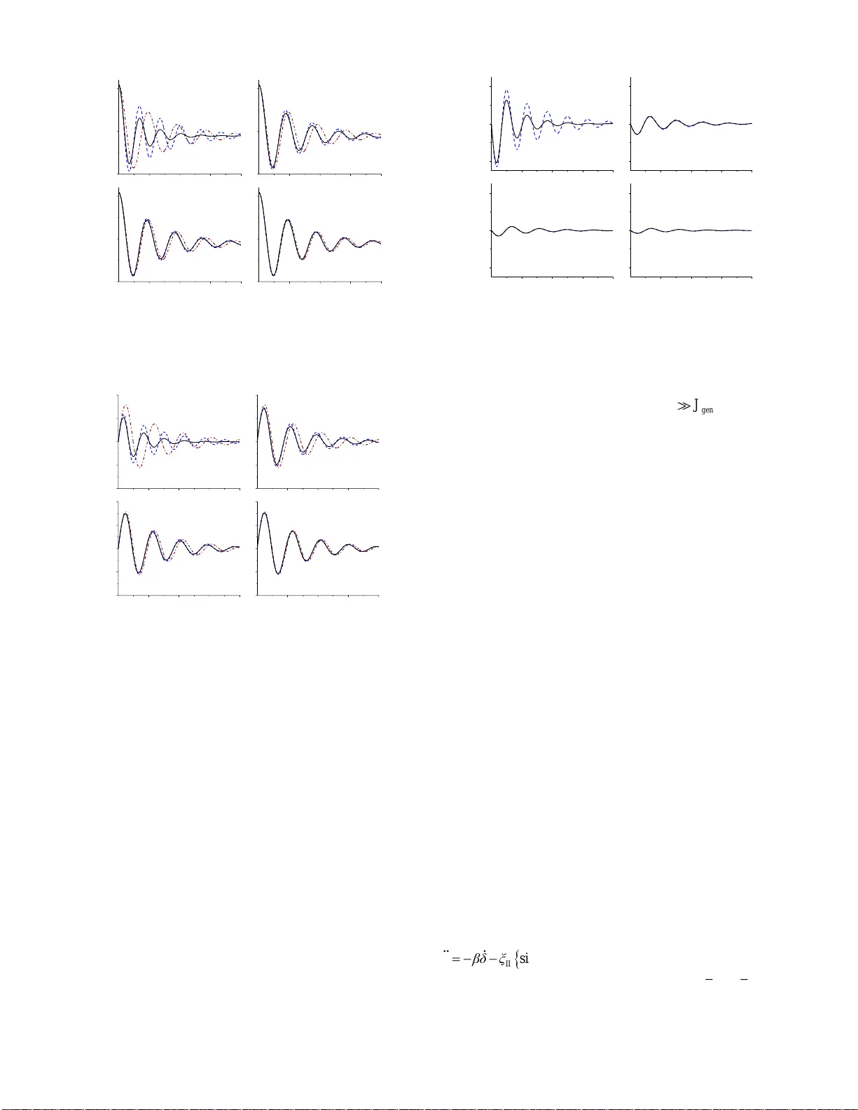
Title: Com parison of coupled nonlinear oscillator models for the transient response of p ower generating sta tions connected t o low inertia sy stems Authors: Mario s Zarifakis, Declan Byrne, William T. Coffey, Yuri P. Kalmykov, Serguey V . Titov, Stephen J. Carrig Published in: IEE E Transactio ns on Power Sy st em s (Early Access) URL: https://ieee xplore.ieee.or g/abstract/doc ument/8782568 Date of Publica tion: 31 July 2019 Print ISSN: 088 5-8950 Electronic ISSN: 1558-0679 DOI: 10.1109/TPW RS.2019.2932376 Publisher: IEEE Funding Agency : Electricity Supply Board; Scienc e Foundation Ireland © 2019 IEEE. Personal use of this material i s perm it ted. Perm i ssio n from IEEE must be obtained fo r all other uses, in any current or future media, including reprinting/re publishing this materia l fo r advertising or promotional purposes, creating new collective works, for resale or redistrib ution to servers or lists, or reuse of any copy righted com ponent of this w ork in other work s. 1 Abs tr a ct — Cou pled no nlin ear o scil la tors , e.g ., Ku ramo to mo del s, are commo nly used to an al yze e lec tri cal power syst ems . The cage m odel from stat isti cal m echani cs ha s also been used to desc ribe the dy nam ics of sync hro nou sly con nec ted gen erat ion sta tion s. Wherea s th e Kura mo to mo del is go od fo r des cribin g hi gh inerti a grid sys tem s, the cage one a llows both h igh an d low in ert ia grid s to be m odel led . Th is is illust rat ed by co mp arin g bo th the s ynchron izat ion tim e and re laxati on t owar ds synch roniz atio n o f eac h mod el b y tr eat ing the ir equ ati ons of m otion in a com mon fram ework roo ted in the dyn ami cs of ma ny coup led pha se osci llat or s. A solu tion of th ese equ at ion s via m atr ix con tinu ed fractio ns is im plem ented ren der in g the cha ract er isti c re laxat ion tim es of a grid -gen era tor sys tem over a w id e ran ge of in ert ia and dam ping. Fo llo wing an ab rup t chan ge in t he d ynam ical s yst em, the power outpu t and bo th gen erator and grid freque nc ies al l exhib it dam ped osci lla tion s n ow dep end ing on the (fin ite) grid iner tia . In prac tic al app lication s, it ap pear s tha t f or a sm all ine rtia system the ca ge m odel is pr efe rable . Index Terms — Power system stability, Power system tr ansients , Power system protection, Ra te of ch ange o f frequency or ROCOF , Renewable energy sources , Synchronous generators. I NT RODUCTION LECTRIC po wer grids have lo ng served as one of the principal motivations f or the s tudy of synchronization phenomena [1]. Nevert heless, the largely unexplored problem of how p ower generat ing stations themselves influence the dynamics o f lo w- inertia po w er grids remains largely unsolved. Since that topic has become pr ogressively more important due to increas ing use of Renewa ble Energy Sources (RES), theoretical studies ro oted in dynamical models of this power g rid-specific problem [ 1],[ 2] are of significa n t interest to Manuscript received xxx, 2019; revised xxx, 201 9 ; accepte d xxx, 2019. Date of publication xx x, 2019. (Correspond ing author: De clan J. Byrne.) S. V. Titov a cknowle dges the Electricity Supply Board for financial support. D. J. Byrne acknowledges Science F oundation I r e land for f inancial sup port. This publication has emanate d fr om rese arch co nducted with the financial support of Science F oundation Ireland under G rant number 17/I FB/5420. M. Zarifa kis and S. J. Carrig are with the Electricity Supply Board, Engineering and Major Projects, Dublin 3, Ireland (e -mail: marios.zarifakis@e sb.ie , stephen.carr ig@esb.ie ). W. T . Coffey an d D. J. Byrne are with th e Department of Electronic and Electrical Enginee ring, Trinity Coll ege, Dublin 2, Ireland (e-mail: wcoffey @mee.tcd.ie ; byne d12@tcd.ie ). Yu. P. Kalmykov is w ith the Laboratoire d e Mathématiques et Physique (EA 4217), Université de Perpig nan Via Domitia, F-66860, Perpignan, F rance (e - mail: kalmykov @univ-perp.fr ). S. V. Titov is with the Kotel’nikov I nstitute of R adio Engineering and Electronics of the Russian A cademy of Sciences, Vvedenskii Square 1, Fry azino, M o scow Region, 141190, Russi a (email: pashkin1212@y andex.ru ). the energy generatio n industr y . Recent publications exist exp loring the effect of increasing grid RES levels on its rotational inertia and dynamics following a distu rbance. This h as usually bee n achieved by f inding relevant physical characteristi cs using simulations on various classical multimachine model testbeds, e.g., si m ulating the dynamic respo ns e [3]-[6], analys ing the eigenvalue sensitivity [4], investigating th e effects on the rate of change of rotor speed [7], and investigating inter-area power-flow oscillations (using a five-machine red uced m od el to represent The Western Electric Coordinating co uncil trans mission grid) [5] . Another method is Koop m an mode deco m position [8],[ 9] which is relevant to the current paper as the nonlinear dynamic response of the s ys tem is represented as a sum o f eigenfunctions i n both cases, although the methods for obtaining them differ significantly. Analysis o f these s ys tems is usuall y per formed via a numerical sol ution of a many b ody s y stem [3] -[7]. To ob t ain analytic results, ho wever, th e many bo dy s ystem must be reduced to a two body o ne, representing two coupled nonlinear phase oscillators. Here o ne ( tagg ed) o scillator models the generator dynamics, w hereas the remainin g generators on the grid are regarded as simply a large inertia oscillator . The latter assumption is merely an idealized rep resentation used to yield two tractable coupled equations. The advantage of th is Ansatz is that the two coupled nonlinear differential eq uations describing the combined dynamics of the generator and grid can be solved analytically. T herefore even a relatively si mple physical m odel may still sug gest qualitative design rules for the network. This can the n be used to reduce th e effects of tra nsient events. Furthermore many methods for analyzing the dynamics of a system of two coupled nonlinear oscillato rs exist. Here we shall co m pare t w o physically acceptab le two-bod y coupled oscillator models, namely, a Kuramoto -like [ 10 ]- [1 2] and a cage m odel [ 13 ],[ 14 ]. Both yield insights into the general phase behavior of a generator connected to a pow er grid with fi nite inertia suc h as prevails in Ir eland. Our solu tion is based on th e transformation of nonlinear differential equatio n s to an infinite system of d ifferential- recurrence equations (see (A3) and ( A 4)) . T his ultimately yields the time dependent dyn amic respo ns e of various characteristics of the ge nerator and grid a s sums o f eigenfunctions (see ( 29 )) . Additionally, t he spectra o f t hese characteristics are describ ed using matrix continued fractio n s. One of th e advantages of our method is that th e results derived are analytic, yielding an intuitive understanding of the Comparison of coupled nonlinear oscillator models for the transient response of power generating stations connected to low inertia systems Marios Zarifakis, D eclan J. By rne, William T. Coffey, Yuri P. Kalm ykov, Serguey V. Titov and Stephen J. Carrig E 2 effects of the n onlinear dynamics on the system. Our solution is based o n the equations o f m otion f or a low inertia grid. Hence , we are not co ns trained by system parameters. Moreo ver, as the solution co mpletely describes the nonlinear dynamics, we can consider any size of fault. Further m o re, our method d oes not require a simulation to b e run. Thus we believe that thi s method will be useful to prac tical en gineers i n the area o f energy generation seeking to anal ys e the dynamics of lo w inertia grids. E QU ATIONS OF M OTI ON FOR THE K URAMOT O - LIKE M ODEL W e first model t h e generator -g rid interactions using Kuramoto oscillators [ 10 ]- [1 2]. Th ese characterize the collective dynamics of many phase oscillator systems and have been used to analyze many dynamical syste m s in p hysics, chemistry, b iology, and engineering rep resenting coup led interacting bodies r otating or torsionall y oscillatin g in time (e.g., chemical reactio ns [1 5], neural ne tw or k s [ 16 ], [ 17 ], coupled Josep hs on junctions [ 18 ], optomechanical s ys tems [ 19 ], laser arrays [ 20 ], and m ean-field qua ntum s ys tems [ 21 ] ). In a po w er grid each machine t y pically op erates with a frequency near the grid reference frequency  = 2  f ( f = 50 or 60 Hz) . Here we describe the dynamics o f t he angles j θ of th e j th ele m ent of the power plan ts (generator and motor) each in accordance w it h a Kuramoto-l ik e model for t h e phase e volution and governed b y the same swing eq uation [ 15 ]     ma x 1 sin , N K j j j j jl j l j l J θ K θ τ θ θ τ         (1) ( 1 , 2,..., ) jN  f or a grid consisting of N units . Here j J are the moments of inertia, K j K are the damping coefficients characterizing the damping to rques o f synchronous machines, ma x ma x jl lj ττ  denotes the electromagnetic torq u e (i.e., the coupling (interaction) strength of t wo machines j and l ), and j τ is th e resulting to rque applied to the generator. Clearly from (1) under n ormal (unperturbed) conditions, all th e generators in the grid operate with the same frequency  . We m a y now reduce (1 ) to a two body proble m as discu ssed in the Introductio n. Here a p articular element , sa y j = N , is designat ed as a generator , i.e., j N gen JJ   , j N gen θθ   , j N g en ττ   , and the remaining machines are then r egarded as identical, i.e., j N grid θθ   and ma x ma x j gen ge n j ττ  . Thus we have     1 ma x 1 sin , , N K gen g e n g e n g e n genl gen grid gen l J θ K θ τ θ θ τ j N           (2)     m ax sin , . K j g r i d j g r i d j gen gri d g en j J θ K θ τ θ θ τ j N        (3) By summing all eq uations (3), we then hav e     11 ma x 11 sin . NN K j g r i d j g r i d j ge n grid gen j jj J θ K θ τ θ θ τ            (4) Equations (2) and (4) can now be rewritten in the simulta neous form:     sin K ge n g e n g e n g e n el ge n grid ge n J θ K θ τ θ θ τ       , (5 )     sin K grid g r i d g r i d g r i d el gr id g en grid J θ K θ τ θ θ τ       , (6) where 1 1 N grid j j JJ     , 1 1 N KK grid j j KK     , 1 1 N grid j j ττ     , 11 11 NN el j gen gen j jj τ τ τ     . Next, we rewrite ( 5) and (6) in the generic f orm     sin K i i i i i j i θ β θ ξ θ θ τ       , (7) where, , i g rid ge n  , , j g en gr id  , / i el i ξ τ J  , / i i i τ τ J  , and in this case, / KK i i i β K J  . If the condition // KK gr id g en grid gen J J K K N  (8 ) is i m posed (i.e., the g rid consists o f N identical generators) then by subtractio n of (7 ) when i=gen f rom ( 7) when i=grid we ha ve the evolution eq uation for the rotor angle (namely the eq uation of motion of a d riven damped pendulum ), viz., s i n δ β δ ξ δ τ    , gri d g en δ θ θ  , (9) where gri d g en ξ ξ ξ  , gri d ge n τ τ τ  , and in this case // K K K K gr id ge n gen ge n gr id g rid β β β K J K J     . T his pendulum model i s also co mmonly use d for the dynamic respo nse of a synchronous ge nerator in an infinite grid [ 22 ],[ 23 ]. N ow , t o describe the effects o f fin ite grid inertia we i ntroduce a ne w variable x , namely the ratio of the grid inertia to th e generator inertia , / gri d ge n x J J  so that in (9)   1 1/ el g en ξ τ x J   ,   1 1/ ge n ge n τ τ x J     , ( 10 ) and x has n o effect on  f or the Kuramoto-like model. Equation (9) can be solved using t he matrix co ntinued fractio n sol ution of the damped pendul um equation (see Appendix), y ielding the general solution of ( 7) for arbitrary K i β , i ξ and i τ . We now seek th e evol ution eq uation for the grid and generator angles in terms o f the rotor angle. Here one must in general solve the (simultaneo us ) system of (5) and (6) . However, by i mposing the condition pro posed in (8) , the solution simplifies. First b y adding (5) and ( 6), w e have   K K K K gri d g r i d g e n g e n g r i d g r i d g e n g e n g r i d ge n J θ J θ K θ K θ K K       ( 11 ) Solving ( 11 ) subject to the condition ( 8) and with (0 ) i θ  , we have 0 gri d g r i d g e n g e n J θ J θ  . ( 12 ) Then by integrating ( 12 ) t w ice subj ect to the init ial co ndition (0 ) i θ  , cor responding to u nperturbed (i.e., stead y ) ro tation of grid and generator , we have     ( ) (0 ) ( ) (0) ( ) , grid grid grid gen gen gen grid gen J θ t θ J θ t θ J J t       ( 13 ) so that the time evolution of t he angles () i θt is explicitly (0) (0) ( ) ( ) grid grid gen ge n ge n grid grid gen grid gen J θ J θ J θ t t δ t J J J J       , ( 14 ) (0) (0) ( ) ( ) grid grid gen gen grid gen grid gen grid gen J θ J θ J θ t t δ t J J J J       . ( 15 ) 3 E QUATIONS OF M OTION FO R THE C AGE M ODEL For comparison, we al so a nalyze the grid and generator dynamics using the alternative cage model [13], [ 14 ], wh ere the dynamics of the a ngles j θ are d escribed by the ma ny body equation     m a x 11 sin NN C j j j l j l j l j l j ll J θ K θ θ τ θ θ τ        . ( 16 ) The essential d ifference bet w een ( 16 ) and ( 1) per tainin g to the Kuramoto-like model i s t hat there [ 12 ] the damping torque is proportional to the deviation of the grid/ge nerator freq u enc y from t he re f erence frequency  , namely   K j j K θ  , w hereas in the cage model [2], [ 13 ] the damping torq u e of the j -th generator (say) is proportio n al to the difference b etween its particular frequency and all o th er generator freq u encies, namely   1 N C jl j l l K θ θ    . The cage (itinerant oscilla tor) model is widely used in c hemical physics ( for a detail ed summary of its app lications see [ 14 ] and references therein) . Following the method used to analyze the K uramoto-like case, we again red uce ( 16 ) to a two body system so that 11 ma x 11 ( ) sin( ) , NN C gen g e n g e n l g e n g r i d gen l ge n grid gen ll J θ K θ θ τ θ θ τ         ( 17 )     11 m a x 11 sin . NN C j g r i d j g e n g r i d g e n j g e n grid ge n j jj J θ K θ θ τ θ θ τ           ( 18 ) Then via the sub stitutions 11 11 NN C C C ge n l j g en lj K K K     , 1 1 N grid j j JJ     , 1 1 N grid j j ττ     , 11 m ax m ax 11 NN el g en l j gen lj τ τ τ     , we have the equation s of m ot ion rendered as     sin C ge n g e n g e n g r i d e l gen grid gen J θ K θ θ τ θ θ τ      , ( 19 )     s in C grid g r i d g r i d g e n e l gri d gen grid J θ K θ θ τ θ θ τ      . ( 20 ) W e now rewrit e ( 19 ) and ( 20 ) as     s i n C i i i j i i j i θ β θ θ ξ θ θ τ      , ( 21 ) where i ξ and i τ ar e defined a s in (7 ) but in t his case / CC ii β K J  . Then b y subtractio n of ( 21 ) when i=gen from ( 21 ) when i=grid we no w have (9) where in this instance CC grid ge n β β β  , or in ter m s of the grid to generator inertia ratio,   1 1/ C ge n β K x J   . ( 22 ) Equation ( 22 ) is ver y important because it e mphasizes the essential difference bet w ee n the cage and Kura m oto-like models for finite inertia grids. To find the evolution eq uation for the grid and generato r angles in terms of the rotor angle, we follow the m ethod for the Kuramoto-like model. B y addition of ( 19 ) and ( 20 ) we again have ( 12 ), thus leading to ( 14 ) and ( 15 ). T R A NSIENT R ESPO NSE F UNCTION Supposing that a disturbance to the motion occurs at the instant 0 t  whereupon the interaction pa rameter el τ alters from an initial value I el τ to II el τ so tha t we require t he transient behavior, starting f ro m an eq uilibrium state I with rotor angle I (0) δδ  to a new equilibrium state II with II () δ t δ    . Both I δ and II δ depend on the app lied torque of the turbine because II I si n / / ge n el gri d el δ τ τ τ τ    and II II II si n / / ge n el gri d el δ τ τ τ τ    . The initial value of I (0 ) δ δ  is zero . To find  ( t ), w e introduce the complete set of function s   II ( ) s i n nq nq at δ δ δ  , ( 23 )     II II ( ) s i n 1 co s nq nq bt δ δ δ δ δ       . ( 24 ) Thus,  ( t ) ca n then b e expressed in terms o f () nq at and () nq bt as 00 II 01 II c o s ( ) ( 1 ( )) c o s ( ) s in δ t b t δ a t δ    , ( 25 ) or 01 ( ) ( ) δ t a t dt    . ( 26 ) We have ( v. A ppendix) from (9) a set of differential-rec u rrence equatio ns governing the evol ution of () nq at and () nq bt (see (A3) and (A4)) . The behavi or of any selected functio n is coupled to that of all the others, so generating an infinite hierarchy o f equations. Numerical solutions for () nq at and () nq bt m ay b e obtained via matrix continued f ractio ns ( v. Appendi x) or else via d irect diagonalization by writing (A3) and (A4) as a first-order matrix differential equation, viz., =0 d dt  C XC . ( 27 ) Here C is the super column vector w it h elements co m prised of the vectors n C and X is the ti m e independent infinite system matrix defined as 11 1 2 2 2 2 3 3 3 44 , ,                              Q Q 0 0 C Q Q Q 0 C C X 0 Q Q Q 0 0 Q Q where the matrices n Q and n  Q and the vector n C are given by (A6) in the Appendix . Equation ( 27 ) can then be solved using the standar d inversion met hods of linear al gebra, i.e., by progressively i ncreasing t he size L o f X until co nvergence is attained. We then have 1 ( ) (0 ) (0 ) tt t e e     X Λ C C U U C , ( 28 ) where 1   Λ U X U is a diagonal matrix with elements composed of all the eigenvalues k λ of X and U reduces X to diagonal form. The columns o f U ar e the co mponents of t he column eigenvectors of t he matr ix X . Equat ion ( 28 ) can then be used to find δt  and δ t  , viz., II ( ) , ( ) , jj L L λ t λ t jj jj δ t c e δ δ t d e       ( 29 ) where j c and j d ar e the elements o f the vectors (v. ( 26 ) and ( 28 )) 4 ma x m a x 1 1 T 1 T 2 3 2 3 ( ) ( ( 0 ) ) , ( ) ( ( 0 ) ) , q q        cU Λ U C d U U C ( 30 ) with max 23 q  U denoting r ow ma x 23 q  of U ( max q is defined in the Appendix). To analy ze the dynamics of system immediately following an alteration of el τ via Fourier transformation, we now introduce the normali zed rotor angle, II I II () () N δ t δ δt δδ    , ( 31 ) describing t h e evolution of () δt from a state I, where (0) 1 N δ  , to the stationary state I I, where ( ) 0 N δt    , after the removal of the disturbance. Analysis of () N δt is preferable in comparison to th at of  ( t ) as it is already nor m alized , viz. (0) 1 N δ  , and has fi nite area under the decay curve . T hus its spectrum (see Fig.1) has no singular points so th at Fourier transformation may be used to analyze it . By one-sided Fourier transformation the se t of dif f erential -recurrence evoluti on equations for () nq at and () nq bt is then c onv erted to a set of algebraic equations for the one-sided Fourier transforms () nq a i ω and () nq b i ω (see Appendix). T hese are solved via matrix continued fractions so yielding a f ormal analytical result for the one-sided Fo u rier trans form of N δt  , viz., 10 I II 0 () 1 ( ) l im ( ) 1 st N N si ω a i ω δ i ω δ t e dt i ω δ δ            . ( 32 ) () N δt can then be recovered from () N δ i ω via inverse Fo urier transformation, v. [2]. Figs. 1 and 2 show the spectr um () N δ i ω and δt  . C HARACTERISTIC F REQUENCI ES AND T IMES If δt  represents a d ecaying oscillatory f unction as exhibited in Fi g. 2, the frequency of the oscillations δ ω of δt  can be roughly esti m ated either from the ( linear) respo n se for small disturbances [24] as 2 II co s / 4 sm ω ξ δ β  , ( 33 ) or from the unda m ped pendu lum equation s i n 0 δ ξ δ   (  =  = 0) yielding [2] 2 ( ) un πξ ω Km  , ( 34 ) where K ( m ) is a co m plete elliptic integral of t he first kind [ 25 ] with modulus 2 0 sin ( / 2) m δ  and 0 δ is the amplitude. T he frequency m a y also be extracted from the spec trum of δt  (see Fig. 1). Fig . 3 shows the behavior of δ ω vs. the parameter II ξ corresponding to the f in al state II. Clearly both d istinct metho ds of estimating the f requency yield similar results. Now, synch ronization dyn amics in p ower-grid ne tw orks is o f great prac tical significance. For example, s y nchro nization o f all power generators in t he sa me interconnection is a n absolute requirement for a power grid to operate. One of the parameters characterizing the sync hronization p rocess is the synchronization time , i.e., the time need ed to recov er synchronized op eration of the grid follo wing a desynchronizatio n event . Thus, we shall use the concept of the integral relaxation tim e of a relaxation function ( from statistical mechanics) to estimate the ti m e scale of a synchronization process. We begin with the Ansatz that a given n ormalized function / () tT N q t e   has exponential behavior with relaxation time T , so that the integral relaxation time may be rigorousl y defined as int 0 () N T q t dt T    . ( 35 ) However, we may also introduce int T for an arbitrary normalized response functio n N δt  which in general is n ot exponentia l [ 13 ] . Th is ti me characterizes t he general p rocess whereby a ph ysical syste m , following cha ng es i n a particular system p arameter, evolv es from one stationary state to another stationary one and there fore may be regarded as a characteristic time o f a synchronization process . Thus i f N δt  simultaneously oscillates and decays, w e can approximate the curve by the envelope crossing all positive m axima as the 0 1 2 3 4 0 1 2 ~ ~ Im[  N ( i w )]  = 0.5, x I = 1, x II = 1.5,  = 0.5 Re[  N ( i w )] w un w sm 0 1 2 3 4 1 0 1 w Fig. 1. Frequency dependence of the real an d imaginary pa rts of () N δ i ω , II I II ( ) ( ) ) / ( ) N δ t δ t δ δ δ     , ( 32 ) , for da m ping paramete r  = 0.5, torque parameter  = 0.5, initial coupling p arame ter I 1 ξ  , and final coupling parameter II 1.5 ξ  . 5 10 -0.5 0.0 0.5 1.0 (d)  I =  /3,  =1, x I =1, x II =5 5 10 15 20 -0.5 0.0 0.5 1.0 q ( t ) (c) t , [s] t , [s]  I =  /3,  =0.3, x I =1, x II =5 p ( t ) 5 10 0.0 0.5 1.0 (b)  I =  /3,  =1, x I =1, x II =2 5 10 15 20 0.0 0.5 1.0 (a)  ( t )  ( t )  I =  /3,  =0.3, x I =1, x II =2 Fig. 2. (Color online) Time dependence of t he function δt  for initial coupling parameter I 1 ξ  and initial angle I /3 δπ  and various values of damping parameters  and final coupling para meters II ξ . Dashed lines: δt  via ( 29 ) . Dotted lines: numerical solution of (9 ). Dashed-dotted lines: exponential approximation for the main maximu m of δt  , viz ., int / I II II ( ) ( ) tT qt δ δ e δ     with int T given by ( 36 ). Solid lines: linear response /2 I II II ( ) ( ) βt pt δ δ e δ     . 5 exponential / () tT N q t e   . Then the integral relaxation time ca n be ap proxim ately e valuated via the time to reach the first maximum int / ( ) ( ) os TT N os N os δ T q T e   at os tT  so that int / ln ( ) os N os T T T δT    . ( 36 ) For a linear respo nse the time of the first m axim um is simply the time interval bet w een two ad jacent m axima , is given by 2/ os δ T πω  , ( 37 ) where δ ω m a y be ap proximated via ( 33 ) , ( 34 ) or else fro m the spectrum of N δt  (see Figs. 1 and 3). Now, for a nonlinear response os T can be ev aluated exactly using ( 29 ) from the smallest nonzero root of 0 δ t    , i.e., 0 j L λt j j de    . ( 38 ) The curve cro ssing all po sitiv e maxima o f () δt is then int / I II II ( ) ( ) tT qt δ δ e δ     . For th e linear respo ns e this curve can be explicitly expr essed as [ 24 ] /2 I I I II ( ) ( ) βt pt δ δ e δ     . R ESULTS AND D ISCUSSI ON Fig . 2 shows the time depend ence of δt  via ( 29 ) for initial coupling I 1 ξ  and initial an gle I /3 δπ  and various values of damping  and final coupling II ξ . By using ( 36 ) we have a rather accurate exponential appr oximation, viz., int / I II II ( ) ( ) tT qt δ δ e δ     f or the m ai n maxim um of δt  . Thus int T can be safely regarded in thi s insta nce as a characteristic time of the relaxation process. Fig. 4 shows the i n tegr al relaxation time extracted via the exponential approxi m ation for the main maxim um o f the relaxation function. Clearly for a highly nonlinea r s ituation (large II I ξξ  and small  ) the approximation ( 37 ) f ails to describe the relaxation effectively. To model the ef f ects of finite grid inertia w e use the definitions of the s y stem parameters i n terms of the grid to generator inertia ratio x , ( 10 ) and for the cage model ( 22 ). The ratio x has no effect on  for the Ku ramoto -like model. Figs. 5- 7 show the tim e dependence of () δt , () gen ωt , and () grid ωt for various x using both the ca ge and Kuramoto-like models. Here () δt is calculated via ( 29 ) and gen g e n ωθ  , grid g r i d ωθ  are calculated via ( 14 ), ( 15 ), and ( 29 ). The m ain effect of the lo w inertia grid is an increase i n the frequency of the oscillatio ns (which ca n b e intuitively p redicted fro m ( 10 ) , ( 33 ), and ( 34 )) . Additionally, the amplitudes of the oscillations of () δt and () gen ωt for the cage model are reduced for low i n ertia ( as expected f rom ( 22 )). For a small, virtually isolated grid like that of Ireland where 10 x , these results ar e highly relevant. C ONCLUSIONS We have presented a comparative study of the electromechanical dynamics o f a generator connected to a low- inertia power grid using coupled p hase oscillators in the form of the cage and Kura m oto models. We conclude that both yield comparable results, wh ich may serve as analytical guidelines for qualitative studies o f the dynamical response of a generator connected for a lo w inertia tra nsmission system . This paper also extends our p revious work o n energ y grid dynamics [2 ] incorpor ating many improveme nts . For example, [2] only considers the dynamics described b y the cage model, whereas here we also treat the dynamics via the Kuramoto -like model (commonly used to analyze grid s ystems [10]- [1 2]) . Als o we have g iven a new d escription of the ti m e dep endent dynamics derived in an ana lytic manner directly fro m the system matrix describing the generator and grid (see ( 27 )-( 30 ) ). Moreover the effects of low grid inertia are now shown explicitly in the equations via a grid to generator inertia ratio (see ( 10 ) and ( 22 )). W e have also provided anal y tic equations describing t he dynamics o f the grid and generato r frequencies (see ( 14 ) , ( 15 ), and ( 29 )). F urthermore w e have introduced different met hods of describing b oth the character istic frequencies and times of the grid -g enerator dynamics following a disturbance (see Sectio n 5). The ad v antage of the Kuramoto -like model is that the damping on a ge nerator can be calculated dir ectly from t h e 0 2 4 6 8 10 0 1 2 3 (a) 1:  1 =  /8 2:  1 =  /4 3:  1 =  /3 w   = 0.5 w  1 2 3 0 2 4 6 8 10 0 1 2 3 (b)  1 =  /3 1:  = 0.1 2:  = 0.6 3:  = 1 x II 1 2 3 Fig. 3. (Colo r onl ine) F requency of oscillation of the relaxation functi on δt  vs. the fi nal coupling parameter II ξ for in iti al coupling parameter I 1 ξ  and various initial angles ( a) I / 8 , / 4 , / 3 δ π π π  and dam ping paramete rs (b)  = 0.1, 0.6, 1. Solid line: un ω , ( 34 ), dashed line: sm ω , ( 33 ) and circles: frequency of maximum value of Re [ ( ) ] N δ i ω (see F ig. 1). 2 4 6 8 10 0 0 1 2 3 4 5 6 1:  = 0.3 2:  = 0.6 3:  = 1 x I = 1,  =0.87 T int x II 1 2 3 Fig. 4. (Color online) I ntegral relaxatio n time int T , ( 36 ) , of th e function q ( t ) v s. final coupling parameter II ξ for torque parameter  = 0.87 initial coupling parameter I 1 ξ  and vario us damping parameters  = 0.3, 0.6, 1 . Solid li nes : δ sm ωω  , ( 33 ); circles: ma x δ ωω  , where max ω i s freque ncy of maximu m value of Re [ ( ) ] N δ i ω (see Fig. 1); d ashed lines: os T via ( 38 ); dott e d l ines: linear response, int 2/ T β  [24]. 6 generator rotor frequency and so does not req u ire know ledge o f the d yn amics o f the grid. This is approp riate if all the generator s in the grid have iden tical frequencies (i.e., frequenc y is synchronized) and th is frequency is constant (and chosen as the reference freque ncy ). This constraint is almost fulfilled in a large-scale power grid (e.g., the Euro pean grid) with high inertia, where t he common frequ ency is so tightly controlled as to be ve ry n ear the nominal frequency . Then usin g the Kuramoto-like model with the nominal frequenc y as the reference frequency i s justified. Ho w ever, t he disadvantage of using this model is tha t it is i nappropriate for analysing sm all inertia systems where t he grid dynamics cannot be so tigh tly controlled. The ad van tage of t he cage model in this i nstance is that it does not r ely at all on the assumption that the grid ha s a constant re ference frequency and therefore is appropriate for analysing these small inertia systems. Moreover, it ca n also be used to anal y ze high inertia grid systems because for infinite grid inertia the damping to inertia ratio coefficient β defined for the ca ge model, 11 () C gri d ge n β K J J   , simply reduces to / C ge n β K J  which is eq uivalent to the Kuramoto-like definition. In a t ypical e nergy grid gri d g e n J J so that b oth solutions will not si gnificantly differ. We have de monstrated ho w the two de gree of freedo m dynamical equations corresponding to bo th models may be solved analytically. The ad v antage o f such sol utions ov er numerical i ntegration metho ds is that t hey yield res ults in closed form, allo w ing one to transparently analyze t he relatio n between the input variables and the response . We have also proposed an accurate technique for calculating the characteristic times of both mod els over a wide range of inertia and friction. T he analytical solution so yielded m ay serve as a basis f or a qualitative understanding of how act ual generat ors behave following a disturbance resulting in a grid- f requen cy change a s well a s revealing m ore general fea tures of co mplex multi-degree o f freedom syste m s. T hey could also be extended to two or m o re grid connected g enerators , or to consider a system o f non-identical generators (b y a veraging over appropriate distribution functions), yielding qua ntitatively better results. Thus we have d emonstrated how lo w ering t he inertia of a grid (e.g., by increasi ng the proportion o f renewable energy sources) may lead to undesirable b ehav ior (see Fig. 7). Therefore w e must also consider methods to counteract such effects, e.g., using Po w er System Stabilizers (PSS) and Automatic Voltage Regulators (AVR) to d am pen the oscillations on the grid. Recently [ 26 ] w e explored this using the co nventional IEEE PSS 1A, where the nonlinear grid- generator d ynamics derived in this pap er (see ( 29 )) are used as inputs to the PSS and A VR. A PPENDIX A. Ma trix Continued Fraction Solution of (9) We rewrite (9) as     I I II II II I I s i n ( ) co s co s( ) 1 sin δ β δ ξ δ δ δ δ δ δ        , ( A 1) where II gr id ge n ξ ξ ξ ξ    and II II si n gr id gen ξ δ τ τ τ    . The time derivatives o f the functions () nq at given by ( 23 ) are 5 10 15 20 0.0 0.5 1.0 5 10 15 20 0.0 0.5 1.0 t , [s] t , [s] 5 10 15 20 0.0 0.5 1.0 (b) x =5 5 10 15 20 0.0 0.5 1.0  ( t )  ( t ) K C / J gen = K K gen / J gen =0.3,  I =  /3,  el I / J gen =1,  el II / J gen =2 (a) x =1 (d) x =20 (c) x =10 Fig . 5 . (Col or online) Time dependence of th e angle  ( t ) for the cage (solid lines) and Kuramoto-like (dashed line s) models and an infinite grid inertia system (dashed-dotted line) for / / 0 .3 , CK gen gen gen K J K J  I / 3 , δπ  I / 1 , el gen τJ  II /2 el gen τJ  and var ious values of the grid inertia to generator i n e r t i a r a t i o x . 5 10 15 20 49.2 49.6 50.0 50.4 50.8 K C / J gen = K K gen / J gen =0.3,  I =  /3,  el I / J gen =1,  el II / J gen =2 5 10 15 20 49.2 49.6 50.0 50.4 50.8 t , [s] t , [s] 5 10 15 20 49.2 49.6 50.0 50.4 50.8 (b) x =5 5 10 15 20 49.2 49.6 50.0 50.4 50.8 w gen ( t ) w gen ( t ) (a) x =1 (d) x =20 (c) x =10 Fig . 6. (Col or online) Time dependen ce of the ge nerator frequen cy () gen ωt for the cage (sol id line) and Kuramoto-like (dashed line) models and an i nf inite grid inertia syste m (d ashed-dot ted line) for / / 0 .3 , CK gen gen gen K J K J  I II I / 3 , / 1 , / 2 el gen el ge n δ π τ J τ J    and various values of the grid in e rtia to generator inertia r atio x . 5 10 15 20 49.6 50.0 50.4 5 10 15 20 49.6 50.0 50.4 t , [s] t , [s] 5 10 15 20 49.6 50.0 50.4 (b) x =5 5 10 15 20 49.6 50.0 50.4 K C / J gen = K K gen / J gen =0.3,  I =  /3,  el I / J gen =1,  el II / J gen =2 w grid ( t ) w grid ( t ) (a) x =1 (d) x =20 (c) x =10 Fig . 7. (Color online) Time dependen ce of the grid frequency () grid ωt fo r the cage (solid lines) and Kuramoto-like (dashed line s) model s for / / 0.3 , CK gen gen gen K J K J  I II I / 3 , / 1 , / 2 el gen el gen δ π τ J τ J    and various values of the gr id inertia to gene rator inertia ratio x . 7       11 I I II II ( ) s i n s i n co s . n q n q nq d a t n δ δ δ δ q δ δ δ δ δ dt       (A2) By sub stituting ( A 1) into (A2), we then have differential - recurrence relations for the () nq at , viz., 1 1 1 1 II 1 1 II 1 II cos sin , n q n q n q n q n q n q d a βna qa qb dt ξ n a δ b δ               (A3) whence 1 1 1 1 II 1 2 II 1 1 II 1 II ( 1 ) sin cos 2 sin . n q nq n q n q n q n q n q d b βnb q a qb dt ξ n a δ b δ b δ                    (A4) Equations (A3) and (A4) can be transfor m ed into the tri - diagonal matrix for m 11 ( ) ( ) ( ) ( ) n n n n n n n d t t t t dt      C Q C Q C Q C (A5) with the initial conditio n s               I II I II I II I II 1 2 I II 2 I II I II 1 1 cos sin sin 1 cos (0) , sin sin 1 cos (0) 0, 2. n δδ δδ δ δ δ δ δδ δ δ δ δ n                            C C Here the infinite column vectors n C and the m atrices n Q and n  Q are 10 10 11 11 0 0 0 0 0 0 0 1 0 0 1 1 0 0 0 , , ( 1 ) , 0 1 0 0 2 0 0 2 2 0 n n n n n n n a b βn a b                                          C Q Q I II II II II II II II II II 0 sin cos 0 0 0 2 sin 0 cos sin 0 0 0 sin cos ( 1 ) 0 0 0 2 sin 0 n δδ δ δ δ δδ ξn δ                           Q (A6) and I is the unit matri x of infinite dimension. Equation (A5) m ay b e solved in the frequency do main via matrix continued fractions [ 13 ],[27]. Using the initial conditions I (0) δδ  and (0 ) 0 δ  and ta king the Laplace transformation of ( A5), we have the following matr ix recurrence relations for () n s C 1 1 2 1 ( ) ( ) ( 0 ) s s s      C Q C C , (A7)   11 ( ) ( ) ( ) 0 n n n n n n s s s s        Q C Q I C Q C , ( n > 1). (A8) The solution of ( A 7) and ( A 8) for () n s C is 1 1 1 ( ) (0 ) s  C Δ C , ( A 9) where n Δ is defined b y the recurrence equation 1 11 n n n n n s         Δ I Q Q Δ Q , (A 10 ) so rep resenting n Δ itself as an infinite m atr ix co ntinued fraction [ 13 ]. Our solutio n is ver y a menable to computation (variou s algorithms for calculating matrix co n tinued fractions are discussed in [ 13 ]). As far as the calculation of the (infinite) n Δ is concerned, we first approximate it by some matrix continued fraction o f finite order (by putting 1 0 n   Q at some n = n max ). Simultaneously, we confined th e di m e nsions of n Q and n  Q to some finite n um ber 2( q max +1). Both n max and q max depend on the model parameters selected and m ust also be chosen tak ing account of the desired degree of accuracy of the calculatio n. We note that the so lu tion of t he damped pendulum eq uation (9) in terms of continued fract ions has been given in [2] via an alternative complete set of relaxation f unctions. However, the new functions () nq at and () nq bt have the significant adva ntages that they are both real, have finite area under th eir curves in the time do m ain and that their Fourier transforms have no singular points. R EFERENCES [1] T. Nishikawa and A. E. Motter, “Comparat ive analysis of existing models for powe r- grid synchron ization”, New J. Phys . vol. 17 , no. 1, p p . 015012, Jan 201 5. [2] M . Zarif akis, W. T. Coffey , Yu. P. Kalmykov, and S. V. Titov, “Mathematical mo dels for the t ransient stability of conve ntional powe r generating stations connected to low in e rtia sy stems”, Eur. Phys. J. Plus , vol. 132, no. 6, p p. 289-301, Jun. 20 17. [3] A. Ulbig, T . S. Borsche, and G. Ander sson, “I mpact of low rotational inertia on power system stability and o peration” in Proc. IFAC World Congr. , vol. 47, no. 3, pp. 7290 – 729, A u g . 2014. [4] S. Eftekharnejad, V. Vittal, G. T. Heydt, B. Keel , and J. L oehr, “Smal l signal stability assessment of powe r s y stems w ith increased penetra tion of photovo ltaic gene ration: A case stu dy,” IEEE Tr ans. Sust ain. Energy , vol. 4, no. 4, pp. 960 – 967, Oct. 2013 [5] G. Chavan, M. W eiss, A. Chakrabortty , S. Bhattachary a, A. Salazar, and F. H abibi- Ashrafi, “I d e ntification an d p re dictive analy si s of a multi-area wecc pow er sy stem model using sy nchrophasors”, IEEE Trans. Smart Grid , vol. 8, no. 4, July 2017. [6] T. Sad amoto, A. Chakrabortty, T. Ishizaki, and J.- I. Imura, “Retrofit control of wind- integrated pow er systems,” IEEE Trans. Power Syst. , vol. 33, no. 3, pp. 2804 – 2815, May 2018. [7] M . Bakh tvar, E. Vittal, K. Z heng, and A. Keane, “Synchronizi ng torque impacts on rotor spee d in power systems”, I EEE T rans. Power Syst. , vol. 32, no. 3, pp. 1 927-1935, May 2017. [8] M . A. Hernández-Orte ga and A. R. Messina, “Nonlinear pow er system analysis using Koopman mode decom position and perturbation t heory ”, IEEE Trans. Pow er Syst. , vol. 33, no. 5, Sept. 2018. [9] A. Mauroy and I. Mezić, “Global stability analy sis using the eigenfunctions o f the Ko opman operator ,” IE EE Trans. A utom. Control , vol. 61, no. 11, p p. 3356 – 3369, Nov. 2016. [10] D. Mani k, M . Rohden, H. Ronellenfitsch, X. Zhang, S. Halle rberg, D. Witthaut, and M . Timme , “Network susceptibil ities: theory and applications”, Phys. Rev. E , vol. 95, n o . 1, pp. 012319-012331, Jan. 2017. [11] J. Machowski, J. Bialek, and J. Bumby, Power System Dynamics, Stability, and C ontrol . New York, USA: John Wil ey & So ns, 2008. 8 [12] G. Filat rella, A. H. Nielse n, and N. F. Pedersen, “Analysis of a power grid using a K uramoto- like model”, Eur. P hys. J. B , vol. 61, no. 4, pp. 485-491, Feb. 2008. [13] W. T. C of fey and Y. P. Kalmykov, The Lange vin Equation , 4th ed. Singapore: World Scientific, 20 17. [14] W. T . Coffey, M. Zarifakis, Yu. P. Kalmykov, S. V. Titov, W. J. Dowling and A. S. Titov, “Cage model of polar fluids: finite cage i ner tia general ization”, J. Chem. Phys ., vol. 147, no. 3, pp. 034509-034517, Jul. 2017. [15] Y. K uramoto, Chemical Os cillations, Wave s, and T urbulence . G ermany, Berlin: Springe r, 1984. [16] H. Sompol insky, D. Golomb, and D. Kleinfeld, “ Global processing of visual stimuli in a neural netw ork of coupled oscillators ” , Proc. Natl. Acad. Sci. U.S.A , vo l. 87 , no. 18, pp. 7200-7204, Se p 1990. [17] C. Kirst, M. T imme, and D. Battaglia, "Dynamic information routing in complex netw orks.", Nat. Commun. , vo l. 7, pp. 11061, Apr 20 16. [18] K. Wiesenfe ld, P. Colet, an d S. H. Strogatz, "Synchronization transitions in a disordered Jose phson series array", Phys. Re v . Lett. , vol. 76 , no. 3, pp. 404-407, Ja n 1996. [19] G. Heinrich, M. Ludw ig, J. Qian, B. Kubala, and F. Marquardt, "Collective dynamics i n optomechanical array s", Phys. Rev. Lett. , vol . 107, no. 4, pp. 04 3603, Jul 2011. [20] A. G. Vladimirov , G. Ko zireff, and P. Mandel, "Sy n chroniz ation of weakly stable oscillators and semiconduc tor lase r arr ays" Europhys. Lett. , vol. 61 , no. 5, pp. 613-619, Mar 200 3. [21] D. Witthaut and M. Timme, "Kuramoto d y n amics in Hamiltonian systems" , Phys. Rev. E , vol. 90 , no. 3, pp. 0 32917, Sep 2014. [22] P. Kundur , Power System Stability and Control . New York, USA: McGraw Hill Inc., 1994. [23] M. Zarifa kis, W.T . Coffey , “ I mpact of el evated Rate of Change o f Frequency (RoCoF) on co nventional powe r generation plant in the I sland of Ireland ” , VGB PowerTech 8 , pp. 47 - 53 , 2014. [24] K.R. Padiyar, Power System Dynamics: Stability and Control , 2nd Ed. India, Hyde rabad: BS Publica tions, 2008. [25] M. Abramowitz and I . A . Stegun (Ed s.), Handb ook of Mathematical Functions . New Yo rk, USA: Dover, 1972. [26] M. Z arifakis, W. T. Coffey, Yu. P. Kalmykov , S. V. Titov, D. J. Byrne, and S. J. Carrig, “ Active damping of power oscillations following frequency changes in low inertia power systems ”, IEEE Tra n s. Power Syst. , in press, A pril 2019. [27] H. Risken, The Fokker – Planc k Equation. Berlin, Ge rmany: Springer, 1984 (Second E dition, 1989).