Leader-Follower Network Aggregative Game with Stochastic Agents Communication and Activeness

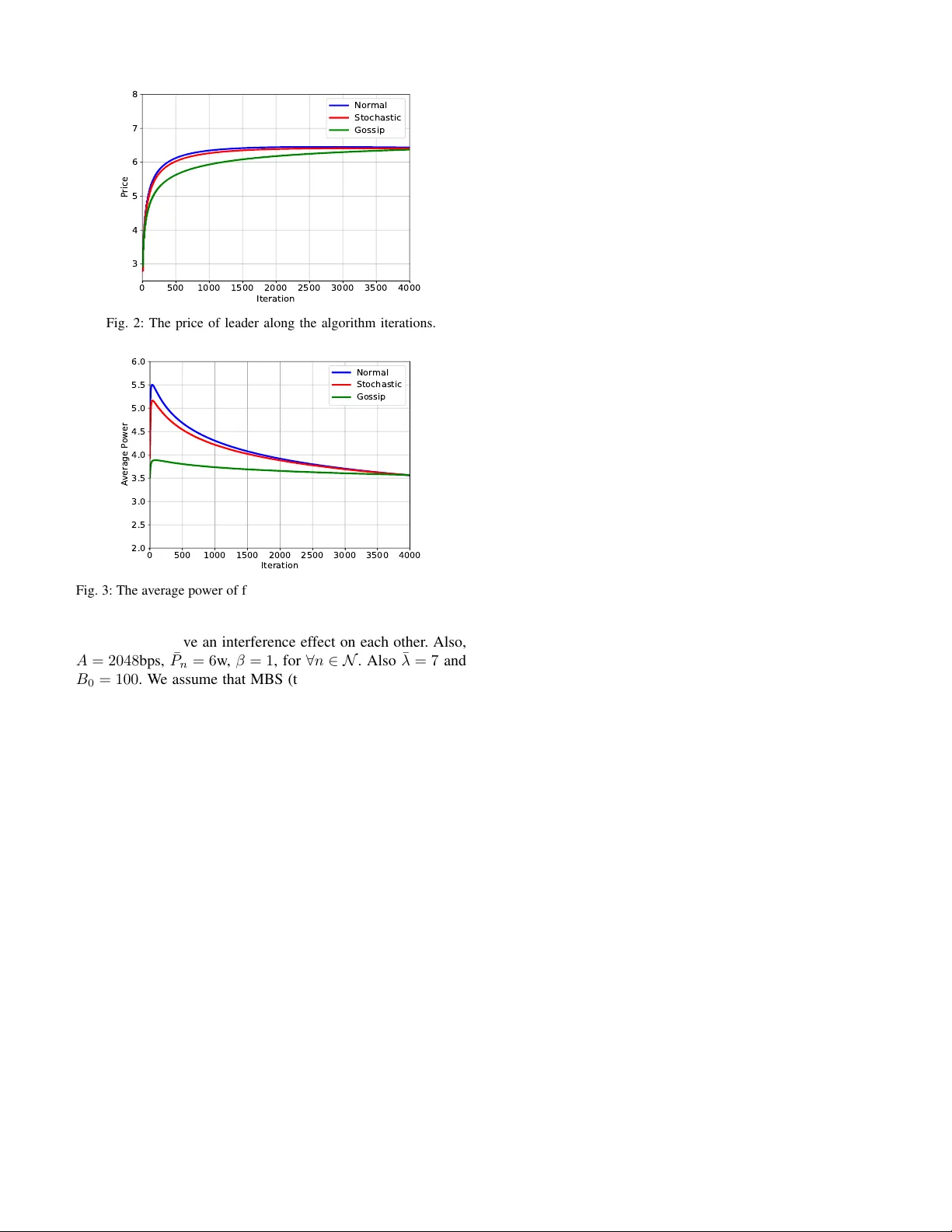
1 Leader -F ollo wer Network Aggre gati v e Game with Stochastic Agents’ Communication and Acti veness Mohammad Shokri, and Hamed K ebriaei, Senior Member , IEEE Abstract —This technical note presents a leader -f ollower scheme for netw ork aggregative games. The f ollowers and leader are selfish cost minimizing agents. The cost function of each follo wer is affected by strategy of leader and aggr egated strategies of its neighbors through a communication graph. The leader infinitely often wakes up and r eceives the aggregated strategy of the follo wers, updates its decision value and broadcasts it to all the followers. Then, the f ollowers apply the updated strategy of the leader into their cost functions. The establishment of information exchange between each neighboring pair of f ollowers, and the activeness of each follower to update its decision at each iteration ar e both considered to be drawn from two arbitrary distributions. Moreover , a distributed algorithm based on sub- gradient method is proposed for updating the strategies of leader and followers. The con vergence of the proposed algorithm to the unique generalized Nash equilibrium point of the game is proven in both almost sure and mean square senses. Index T erms — Network aggregati ve game, leader -follower , stochastic network, sub-gradient method, distrib uted algorithm. I . I N T RO D U C T I O N Distributed optimization over networks has attracted widespread attention of researchers in recent years [1]. As a typical framework, each agent in a network aims to minimize a social or an individual cost function while it communicates with some other agents through the network. In case that each agent is modeled as a selfish player who aims to minimize its own cost and also, the agent’ s cost is affected by decision variables of its neighbors through the network topology , the problem can be studied as a non-cooperativ e network game [2]. If the effect of decision variables of riv als on the agent’ s cost function appears as an aggregativ e term (e.g. summation or weighted sum), the network game is known as network aggregati ve game (N A G) [3]. Man y applications can be studied via this frame work including, power system [4], opinion dynamics [5], communication system [6], provision of public goods [7] and criminal networks [8]. In a class of N A Gs, the cost function of each agent is affected by the aggregated strategies of all network agents [9]– [11] (including neighbors and non-neighbors). In this case, the coupling term among the agents is the same for all of them. This assumption does not cover the problems that agents hav e dif ferent relev ancy or limited communication capabilities. Such challenges motiv ate studying another type of NA Gs in which agents ha ve their dependency with their neighbors. In [12], N A Gs are studied for the agents with quadratic cost functions. Therein, some algorithms are proposed which M. Shokri and H.Kebriaei are with the School of Electrical and Computer Engineering, College of Engineering, Univ ersity of T ehran, Iran. (email: mo.shokri@ut.ac.ir , kebriaei@ut.ac.ir) con verge to the Nash equilibrium point using the best response functions while at each iteration, agents communicate with their neighbors and update their strategies. Furthermore, in [13], a Nash seeking dynamics is utilized for agents with proximal quadratic cost functions whose best responses are in the form of proximal operator . In [14], the cost function of the agents is considered in general form. In this work, a distributed algorithm has been utilized in which each agent communicates with all its neighbors at each iteration and updates its strategy based on its best response function. Howe ver , the algorithms are designed based on the best response scheme which imposes high computational complexity , specially for a general cost function. In such a case, as mentioned in [15], the players naturally dismiss strategies which are characterized by high computational cost and hence, the gradient response seems to an appropriate choice for updating the decision of the agents [16]. In the mentioned researches on N A Gs, all the agents are in the same order of decision making with the same "structure" of cost functions and communication type. Howe ver , in many applications, there is a high-le vel agent (leader) who aims to optimize its own objective function which also depends on the strategies of other agents at a lower lev el (followers). Se veral researches hav e in vestigated leader -follower games [17]–[19] and it has been extensi vely utilized in many engineering fields such as wireless sensor networks [20], supply chain management [21], and smart grid [22]. If the leader has complete information about the followers’ cost functions, then the concept of Stackelberg equilibrium can be applied directly [18]. In this case, the problem can be solved as a bi-level optimization in which the leader first computes the reaction function of the followers with respect to its strate gy . Then, by applying the reaction function of the followers into its own cost function, the leader finds its optimal strategy . Howe ver , if the leader does not hav e a-priori information about the cost function of the followers, then the leader needs to learn its optimal strategy by iterativ e methods. In [17], a leader- following problem is discussed in which the cost function of the leader is independent of the followers’ strategies and only the followers respond to leaders’ strategy . In [19], an iterative hierarchical mean-field game is studied including a leader and a large number of followers. The leader first announces its decision and then, follo wers respond by knowing the leader’ s decision. In this paper , we propose a leader-follo wer NA G. The leader has a different type of cost function from the follo wers which is affected by the aggregated strategy of all the followers. Additionally , the leader has a different type of communication and acti veness from the followers. It is considered that the 2 leader infinitely often: wakes up, receives the last aggreg ated strategy of follo wers, updates its strategy , broadcasts it to all the follo wers, and then goes to sleep. In the lower level, the followers receiv e the last decision value of the leader and play a N A G until the next decision update of the leader . The cost function of each follo wer is affected by aggregated strategies of its neighbors and also the strate gy of the leader . W e also consider stochastic communication and activ eness of the agents in N AG. At each arbitrary iteration, based on a stochastic binary distribution, each follower may become activ e to update its decision based on the projected sub- gradient method. Besides, at each iteration, an agent may receiv e the decision value of a neighboring agent based on another stochastic binary distribution. The corresponding stochastic binary v ariables of the two mentioned distrib utions can be dependent on each other , and further , there might be some constraints on those variables. Finally , a distributed algorithm is proposed in which the decision values of the leader and followers con ver ge to the unique Generalized Nash Equilibrium (GNE) point of the game. T o the best of our knowledge, compared to single-lev el N A Gs [12]–[14], this is the first paper that proposes a leader - follower scheme for N AGs. Further, this is the first paper that presents a general stochastic frame work that simultaneously considers communication and acti veness of the agents in N A Gs in which the Gossip based communication protocol [23] can be encountered as a special case of the proposed frame- work. From other aspects, compared to aggregati ve games which consider the av erage strategy of whole population as a common coupling term among the agents [9]–[11], in this paper , the local aggre gativ e term is studied in which only neighbors of each follower , as well as the leader, af fect the follower’ s cost function. Compared to the literature of NA Gs, those consider the local aggregati ve term, we have studied a general strongly con vex cost function instead of quadratic one [12], [13]. In contrast with the papers which have utilized the best response dynamics as the agents’ decision update rule [12]–[14], we hav e used the projected sub-gradient method for optimization to cope with the limited computational capa- bilities of the agents. The main contributions of this paper can be summarized as follo w: • W e propose a leader-follo wer framework for N A G. • W e study stochastic communication and activeness of the agents in NA G. • A distributed algorithm based on projected sub-gradient method is proposed and its con ver gence to the unique GNE point of the game is prov en in both almost sure and mean square senses. This paper is structured as follows. The system model is introduced in Section II. In Section III, communications frame- work and information structure are gi ven and a distributed optimization algorithm is proposed for decision making of the agents. The conv ergence of the algorithm to the GNE point of the game is proven in Section IV. Simulation results are presented in Section V. Finally , Section VI summarizes the results and draws conclusion. N OTA T I O N A N D P R E L I M I N A R I E S N and R are the set of natural and real numbers, re- spectiv ely . |N | denotes the number of members of the set N . Let A > denotes the transpose of a vector/matrix A . || A || indicates the matrix norm which is equal to the largest eigen value of the matrix. The 2-norm of vector x is defined by k x k = √ x > x . col ( x 1 , ..., x N ) = [ x > 1 , ..., x > N ] > indicates the column augmentation of column vectors x n for n = 1 , ..., N . ~ 1 n = col (1 , ..., 1) and ~ 0 n = col (0 , ..., 0) where ~ 1 n , ~ 0 n ∈ R n . The probability function and expected v alue are denoted by P { . } and E { . } , respecti vely . Supposing the function f ( . ) : X → R , g ( x 0 ) is called the sub-gradient of f ( . ) at x 0 if ∀ x ∈ X : f ( x 0 ) + ( x − x 0 ) > g ( x 0 ) ≤ f ( x ) . Also, the projection operator of X is defined by Π X ( x ) = arg min y ∈X || y − x || 2 . g ( x ) is strictly monotone if ( g ( x 2 , r ) − g ( x 1 , r )) > ( x 2 − x 1 ) > 0 for ∀ x 1 , x 2 : x 1 6 = x 2 . I I . S Y S T E M M O D E L Consider a set of follower agents N = { 1 , ..., N } and a leader in volv ed in a non-cooperativ e game. The followers are connected to each other via a communication network repre- sented by a directed graph G ( N , A ) where A = [ a nm ] n,m ∈N is adjacency matrix of G such that a nm = 1 if there is a communication link from follower m to n , and a nm = 0 otherwise (more details on communication network of the followers is given in Section III-A). Each follower n ∈ N has its decision variable (i.e. strategy) x n ∈ X n where X n ⊂ R M F is a non-empty , compact and con vex set. The cost function of follower n depends on the aggregated strategy of its neighbors whose set is denoted by N n , and also the strate gy of the leader . Therefore, the cost function of follower n is defined as follows J F n ( x n , σ n ( x − n ) , y ) : x n ∈ X n (1) where x − n = col ( x 1 , ..., x n − 1 , x n +1 , ..., x N ) , and y ∈ Y is the strategy of leader which is selected from a compact and con vex set denoted by Y ⊂ R M L . Also, we define d n ( x n , σ n ( x − n ) , y ) as a sub-gradient of J F n ( x n , σ n ( x − n ) , y )) with respect to x n . σ n ( x − n ) is the aggregated strategy of follower - n ’ s neighbors which is defined as σ n ( x − n ) = X m ∈N n w nm x m . (2) where P m ∈N −{ n } w nm = 1 , w nm > 0 if a nm = 1 , and w nm = 0 if a nm = 0 . Hence, we can define the weight matrix of the graph G by W = [ w nm ] n,m ∈N . The cost function of the leader is defined as follo ws J L ( y , σ 0 ( x N )) : y ∈ Y . (3) Further , d 0 ( y , x N ) denotes a sub-gradient of J L ( y , σ 0 ( x N )) with respect to y . The cost function of leader is also affected by the aggregated strategy of the followers σ 0 ( x N ) defined by σ 0 ( x N ) = X n ∈N w 0 n x n (4) where x N = col ( x 1 , ..., x N ) , w 0 n denotes the weight of bidirectional communication link between follower n and the 3 leader , and we hav e P n ∈N w 0 n = 1 , and w 0 n ≥ 0 . let ~ w 0 = col ( w 01 , ..., w 0 N ) denotes the leader weight vector . Accordingly , the non-cooperativ e game among the followers and leader is defined as follo ws G =            Players: follo wers N and the leader Strategies:  Follo wer n : x n ∈ X n Leader: y ∈ Y Cost:  Follo wer n : J F n ( x n , σ n ( x − n ) , y ) Leader: J L ( y , σ 0 ( x N )) (5) Assumption 1: J F n ( x n , σ n ( x − n ) , y ) and J L ( y , σ 0 ( x N )) are sub-differentiable and strongly con vex over X n and Y with respect to x n and y , respectiv ely . i.e. there exist C n and C 0 for ∀ n ∈ N such that ( d n ( x n , σ, y ) − d n ( x 0 n , σ, y )) > ( x n − x 0 n ) ≥ C n || x n − x 0 n || 2 ( d 0 ( y , σ ) − d 0 ( y 0 , σ )) > ( y − y 0 ) ≥ C 0 || y − y 0 || 2 (6) Also, there exist Lipschitz constants L and L 0 such that ∀ n ∈ N , ∀ x n ∈ X n , y ∈ Y , ∀ σ 1 , σ 2 ∈ { σ n ( x − n ) | x − n ∈ Q m 6 = n X m } , we have || d n ( x n , σ 1 , y 1 ) − d n ( x n , σ 2 , y 2 ) || ≤ L || σ 1 − σ 2 || + L || y 1 − y 2 || || d 0 ( y , σ 1 ) − d 0 ( y , σ 2 ) || ≤ L 0 || σ 1 − σ 2 || (7) where d n ( x n , σ n ( x − n ) , y ) and d 0 ( y , σ n ( x − n )) are the sub- gradients of J F n and J L , respectiv ely .  The equilibrium point of the aforementioned leader-follo wer game is defined as follo ws: Definition 1: ( x ∗ N , y ∗ ) is a Generalized Nash equilibrium (GNE) point of the leader-follo wer game between the follo w- ers and the leader if ∀ x n ∈ X n : J F n ( x ∗ n , σ ( x ∗ − n ) , y ∗ ) ≤ J F n ( x n , σ ( x ∗ − n ) , y ∗ ) ∀ y ∈ Y : J L ( y ∗ , σ 0 ( x ∗ N )) ≤ J L ( y , σ 0 ( x ∗ N )) (8) ∀ n ∈ N where x ∗ − n = col ( x ∗ 1 , ..., x ∗ n − 1 , x ∗ n +1 , ..., x ∗ N ) and x ∗ N = col ( x ∗ 1 , ..., x ∗ N ) .  I I I . T H E L E A D E R - F O L L O W E R N E T W O R K G A M E A. Communication and Information Structure 1) Follo wers’ Communication and Activeness: W e consider that follower n receiv es information of its neighbor m ∈ N n at iteration k with probability p k mn . Furthermore, the follower n is activ e at iteration k to update its decision with probability q k n . Let random binary variables l k n,m and e k n denote the establishment of communication from follower n to m , and activ eness of follower n at iteration k , respectively . Clearly , ∀ k ≥ 0 : l k n,m = 0 for non-neighbor followers ( a nm = 0 ). Then, the last information of follower n from follower m denoted by ˜ x k n,m is updated as follo ws: ˜ x k +1 n,m = (1 − l k n,m ) ˜ x k n,m + l k n,m x k m . (9) Based on (9), the aggregated strategy of neighborhoods of follower n at iteration k is calculated as ˜ σ k n = σ n ( ˜ x k n, − n ) where ˜ x k n, − n = col ( ˜ x k n, 1 , ..., ˜ x k n,n − 1 , ˜ x k n,n +1 , ..., ˜ x k n,N ) . Let’ s consider L k = [ l nm ] n,m ∈N and E k = col ( e k 1 , ..., e k N ) as the connecti vity matrix and the acti vity v ector of the followers at iteration k , respectiv ely . The constraint set P represents the set from which L k and E k are selected for all iterations ∀ k ≥ 0 . Further , H k denotes the history set of stochastic variables L k and E k up to iteration k which is defined by H k +1 = H k ∪ { ( L k , E k ) } and H 1 = { ( L 0 , E 0 ) } . In this paper , the probabilities of L k and E k are considered to be possibly dependent to H k and P as follows: P { l k nm = 1 |F k } = p k nm , P { e k n = 1 |F k } = q k n (10) where F k = H k ∩ P . Apparently , F k ⊂ F k +1 holds for ∀ k ≥ 0 . T o illustrate the dependency among stochastic v ariables, in what follows, the well-kno wn Gossip-based communication protocol [23] has been studied as an example of the proposed communication framew ork. Example 1 (Gossip-based Communication): Suppose that the follo wers communicate to each other through an undirected graph G ( N , A ) . In gossip-based communication, each node has an independent stochastic clock which ticks with rate 1 Poisson process and makes the corresponding agent become activ e. The simultaneous clock ticks are neglected and as a result, at most one agent wakes up at each time slot of global clock. For instance, at k th time slot, let the clock of agent n ticks. It wakes up and contacts with only one neighbor (say agent m ). They communicate with each other , update their strategies and then both go to sleep. In this case, our communication frame work imposes the following constraints: P =  ( L k , E k )     X n ∈N e k n = 2 , l k nm = e k n e k m , e k n e k m ≤ a nm , ∀ n, m ∈ N  (11) The first constraint indicates that only two player could be activ e in iteration k . l k nm = e k n e k m implies that a link is established when both of its sender and receiver are activ e. In addition, l k nm = l k mn can be concluded from this constraint. Furthermore, inequality constraint e k n e k m ≤ a nm prev ents two non-neighbors to become active. The probability of each link and each node are calculated as follows: p k nm = 1 N ( 1 |N n | + 1 |N m | ) , q k n = 1 N (1 + X m ∈N n 1 |N m | ) (12) where N n = { m | a mn = 1 } .  Assumption 2: There exist γ > 0 and δ > 0 such that p nm ≥ γ and q n ≥ δ for ∀ n ∈ N , ∀ m ∈ N m .  Note that p nm = 0 for ∀ n ∈ N , ∀ m / ∈ N m . 2) Communication between leader and followers: It is assumed that the leader does not exchange information with the followers at ev ery iterations. Instead, it is considered that the leader infinitely often wakes up and receiv es aggregated strategy of the followers in an arbitrary desired iteration set K L = { k L i } ∞ i =0 . The leader also updates its decision v ariable and broadcasts it to all the followers at the same iteration. It is supposed that k L 0 = 0 . Assumption 3: There is ¯ K < ∞ such that k L i +1 − k L i ≤ ¯ K for ∀ i ∈ N .  4 F3 F2 F1 F5 F4 L Fig. 1: The information scheme of leader-follower network game between followers ("F" shapes) and the leader ("L" shape). The filled and unfilled objects indicate the acti ve and inactive agents to make decision, respectiv ely . The dashed line indicates that there exists a communication line, but it’ s not establish at iteration k . The schematic of information flows among followers and between followers and leader is sho wn in Fig. 1. Each information exchange among followers could be established stochastically ∀ n, m ∈ N . B. Decision Making In this paper , the projected sub-gradient method is utilized for decision making of each follo wer as follo ws x k +1 n = Π X n ( x k n − e k n α k n g k n ) (13) where g k n = d n ( x k n , ˜ σ k n , y k ) and α k n is the step size of follower n at iteration k . Clearly , x k n is not updated if e k n = 0 . Also, the leader updates its strategy at k ∈ K L as follows y k +1 = Π Y ( y k − α k 0 g k 0 ); ∀ k ∈ K L y k +1 = y k ; ∀ k / ∈ K L (14) where g k 0 = d 0 ( y k , σ k 0 ) and α k 0 is the step size of the leader at iteration k . W ithout loss of the generality , we set α k +1 0 = α k 0 , ∀ k / ∈ K L . In this paper , the following assumptions are considered for the step sizes of the players. Assumption 4: α k n , ∀ n ∈ N ∪ { 0 } are Non-increasing, P ∞ k =0 α k n = ∞ , and P ∞ k =0 ( α k n ) 2 < ∞ .  Assumption 5: There exists κ such that α k ≤ κα k where α k = max ( α k 1 , ..., α k N , α k 0 ) and α k = min ( α k 1 , ..., α k N , α k 0 ) .  The optimization procedure for the leader-follo wer network game is presented in Algorithm 1. Based on Algorithm 1, the leader makes decision at iterations k L i ∈ K L and waits in other iterations, while the followers are making decision. In other words, the follo wers continue their interactions and decision makings based on the last informed decision of the leader for some iterations, until the next decision of the leader is announced. The initial values of the parameters are chosen from their feasible re gion. I V . C O N V E R G E N C E A N A L Y S I S In this section, the con ver gence of Algorithm 1 to the unique GNE point of G is studied. Under Assumption 1, as a result of strong con ve xity of the cost functions, there exists a GNE point Algorithm 1 The leader -follower network game algorithm Initialize x n , y and ˜ x nm for ∀ n, m ∈ N and k ← 0 Iteration Leader : σ 0 ← σ 0 ( x N ) g 0 ← d 0 ( y , σ 0 ) y ← Π Y ( y − α k 0 g 0 )) Repeat Follo wer n ∈ N : If e k n = 1 : ˜ σ n ← σ n ( ˜ x n, − n ) g n ← d n ( x n , ˜ σ n , y ) x n ← Π X n ( x n − α k n g n ) update ˜ x nm via (9) based on l k nm k ← k + 1 Until k ∈ K L z ∗ = ( x ∗ N , y ∗ ) for G [24]. Before discussing the con vergence, we propose the follo wing lemmas: Lemma 1 (Theor em 1 of [25]): Let z k , β k , η k , and ζ k be non-negati ve F k -measurable random variables. Also, assume that F k is σ -algebra and F k ⊂ F k +1 holds for ∀ k ≥ 0 . If P ∞ k =0 β k and P ∞ k =0 η k almost surely conv erge, and the following equation E { z k +1 |F k } ≤ (1 + β k ) z k + η k − ζ k (15) holds, then z k and P ∞ k =0 ζ k < ∞ almost surely con ver ge.  Lemma 2: || x k +1 n − x k n || ≤ A n α k n for ∀ n, m ∈ N where || d n ( x n , σ, y ) || ≤ A n , ∀ x n ∈ X n .  Pr oof: See Appendix A. Lemma 3: P ∞ k =0 α k n || ∆ ˜ x k nm || < ∞ for ∀ n, m ∈ N in almost sure sense where ∆ ˜ x k nm = ˜ x k nm − x k m .  Pr oof: See Appendix B. Using lemmas 2 and 3 , the con vergence of Algorithm 1 is prov en in Theorem 1. Theor em 1: Consider Assumptions 1, 2, 3, 4 and 5. If the constants C n and C 0 in (6) satisfy C n > κ δ ¯ L and C 0 > κ ¯ K ¯ L ∀ n ∈ N , Algorithm 1 almost surly con verges to the GNE point of the leader-follo wer game where ¯ L = max (2 L, L 0 ) .  Pr oof: Consider the notation ∇ x k n = x k n − x ∗ n . Based on Proposition 1.5.8 of [26], x ∗ n = Π X n ( x ∗ n − e k n α k n d n ( x ∗ n , σ ∗ n , y ∗ )) where σ ∗ n = σ n ( x ∗ − n ) . Since the projec- tion operator Π X n ( . ) is non-expansiv e and e k n ≤ 1 , we have ||∇ x k +1 n || 2 ≤ ||∇ x k n − e k n α k n  d n ( x k n , ˜ σ k n , y k ) − d n ( x ∗ n , σ ∗ n , y ∗ )  || 2 = ||∇ x k n || 2 + ( e k n α k n ) 2 || d n ( x k n , ˜ σ k n , y k ) − d n ( x ∗ n , σ ∗ n , y ∗ ) || 2 − 2 e k n α k n  d n ( x k n , ˜ σ k n , y k ) − d n ( x ∗ n , σ ∗ n , y ∗ )  > ∇ x k n ≤ ||∇ x k n || 2 + 4 A 2 n ( α k n ) 2 − 2 e k n α k n Ψ k n − 2 e k n α k n  d n ( x k n , ˜ σ k n , y k ) − d n ( x k n , σ k n , y k )  > ∇ x k n (16) where Ψ k n =  d n ( x k n , σ k n , y k ) − d n ( x ∗ n , σ ∗ n , y ∗ )  > ∇ x k n , σ k n = σ n ( x k − n ) . Let consider that || x 1 − x 2 || ≤ B n for ∀ x 1 , x 2 ∈ X n . 5 According to Assumption 1, we hav e − e k n α k n  d n ( x k n , ˜ σ k n , y k ) − d n ( x k n , σ k n , y k )  > ∇ x k n ≤ α k n L || ˜ σ k n − σ k n ||||∇ x k n || ≤ LB n α k n || ˜ σ k n − σ k n || ≤ LB n α k n X m ∈N n w nm || ∆ ˜ x k nm || . (17) Therefore, by putting (17) into (16), we have ||∇ x k +1 n || 2 ≤ ||∇ x k n || 2 + 4 A 2 n ( α k n ) 2 − 2 e k n α k n Ψ k n + 2 LB n α k n X m ∈N n w nm || ∆ ˜ x k nm || ≤ ||∇ x 0 n || 2 + 4 A 2 n k X k 0 =0 ( α k 0 n ) 2 − 2 k X k 0 =0 e k 0 n α k 0 n Ψ k 0 n + 2 LB n X m ∈N n w nm k X k 0 =0 α k 0 n || ∆ ˜ x k 0 nm || (18) Suppose the notation ∇ y k = y k − y ∗ . Considering the leader’ s decision at leader’ s iteration k L j , and following the same operation from (16) to (18), we have ||∇ y k L j +1 || 2 ≤ ||∇ y k L j || 2 + 4( α k L j 0 ) 2 A 2 0 − 2 α k L j 0 Ψ k L j 0 ≤ ||∇ y 0 || 2 + 4 j X i =0 ( α k L i 0 ) 2 A 2 0 − 2 j X i =0 α k L i 0 Ψ k L i 0 . (19) where Ψ k 0 =  d 0 ( y k , σ k 0 ) − d 0 ( y ∗ , σ ∗ 0 )  > ∇ y k , σ k 0 = σ 0 ( x k N ) , σ ∗ 0 = σ 0 ( x ∗ N ) and || d 0 ( y , σ 0 ) || ≤ A 0 . Now , let define Φ j = ||∇ y k L j − 1 +1 || 2 + P n ∈N ||∇ x k L j − 1 +1 n || 2 . Therefore, using inequalities (18) and (19), we hav e: E { Φ j +1   F k L j } ≤ Φ j + 4( α k L j 0 ) 2 A 2 0 + 4 X n ∈N A 2 n X k 0 ∈K 0 j ( α k 0 n ) 2 + 2 L X n ∈N X m ∈N n B n w nm X k 0 ∈K 0 j α k 0 n || ∆ ˜ x k 0 nm || − 2 α k L j 0 Ψ k L j 0 − 2 X n ∈N X k 0 ∈K 0 j α k 0 n E { e k 0 n   F k 0 } Ψ k 0 n . (20) where K 0 j = { k L j − 1 + 1 , . . . , k L j } . Based on definition of Ψ k 0 n , and adding and subtracting the term d n ( x ∗ n , σ k 0 n , y k 0 ) , we have Ψ k 0 n =  d n ( x k 0 n , σ k 0 n , y k 0 ) − d n ( x ∗ n , σ k 0 n , y k 0 )  > ∇ x k 0 n +  d n ( x ∗ n , σ k 0 n , y k 0 ) − d n ( x ∗ n , σ ∗ n , y ∗ )  > ∇ x k 0 n . (21) Based on strongly conv exity and Lipschitz property in As- sumption 6, we ha ve − α k 0 n e k 0 n Ψ k 0 n ≤ − α k 0 n e k 0 n C n ||∇ x k 0 n || 2 + α k 0 n L  ||∇ y k L i || + || σ k L i 0 − σ ∗ 0 ||  ||∇ x k 0 n || . (22) Now , using Assumptions 5, we can write (22) as follo ws − α k 0 n e k 0 n Ψ k 0 n ≤ − α k 0 C n e k 0 n ||∇ x k 0 n || 2 + α k 0 κL ||∇ x k 0 n || ( ||∇ y k 0 || + X m ∈N n w nm ||∇ x k 0 m || ) . (23) By following the same procedure for the leader , we have − α k L j 0 Ψ k L j 0 ≤ − α k L j C 0 ||∇ y k L j || 2 + α k L j L 0 X n ∈N w 0 n ||∇ x k L j n ||||∇ y k L j || . (24) Considering Assumption 2, it’ s clear that E { e k 0 n   F k 0 } = q k n ≥ δ . Therefore, applying inequalities (23) and (24) into the last two terms of (20), it can be concluded that − α k L j Ψ k L j 0 − X n ∈N X k 0 ∈K 0 j α k 0 n E { e k 0 n   F k 0 } Ψ k 0 n ≤ − α k L j C 0 ||∇ y k L j || 2 − X n ∈N X k 0 ∈K 0 j δ α k 0 C n ||∇ x k 0 n || 2 + X k 0 ∈K 0 j α k 0 v k 0 > V k 0 v k 0 . (25) where v k 0 = col ( ||∇ x k 0 1 || , ..., ||∇ x k 0 N || , ||∇ y k 0 || ) and V k 0 =         L W L ~ 1 N L 0 ~ w > 0 0  k 0 ∈ K L  L W L ~ 1 N ~ 0 > N 0  k 0 / ∈ K L It is straightforward to see that the summation of each ro w of the matrices  L W L ~ 1 N  and  L 0 ~ w > 0 0  are equal to 2 L and L 0 , respectiv ely . Therefore, based on Perron-Frobenius Theorem [27], ||V k 0 || ≤ max (2 L, L 0 ) and ||V k 0 || ≤ 2 L for k 0 ∈ K L and k 0 / ∈ K L , respectiv ely . Hence, v k 0 > V k 0 v k 0 ≤ ¯ L || v k 0 || 2 for ∀ k 0 ≥ 0 . Therefore, X k 0 ∈K 0 j α k 0 v k 0 > V k 0 v k 0 ≤ X k 0 ∈K 0 j α k 0 ¯ L ||∇ x k 0 n || 2 + α k L j ( k L j − k L j − 1 ) ¯ L ||∇ y k L j || 2 . (26) where the last term of (26) is rearranged, since the leader only makes decision at k L j ∈ K L and therefore, the term ||∇ y k L j || 2 is the same from iteration k L j − 1 to k L j . By putting (25) and (26) into (20), it can be concluded that E { Φ j +1   F k L j } ≤ Φ j + 4( α k L j 0 ) 2 A 2 0 + 4 X n ∈N A 2 n X k 0 ∈K 0 j ( α k 0 n ) 2 | {z } T j 1 + 2 L X n ∈N X m ∈N n B n w nm X k 0 ∈K 0 j α k 0 n || ∆ ˜ x k 0 nm || | {z } T j 2 − 2 α k L j ( C 0 − κ ( k L j − k L j − 1 ) ¯ L ) ||∇ y k L j || 2 | {z } T j 3 − 2 X n ∈N X k 0 ∈K 0 j α k 0 ( δ C n − κ ¯ L ) ||∇ x k 0 n || 2 | {z } T j 4 . (27) Based on Assumption 4, P ∞ j =0 T j 1 is bounded. Also, based on Lemma 3 we have P ∞ j =0 T j 1 < ∞ . According to As- sumption 3, C 0 − ( k L j − k L j − 1 ) κ ¯ L ≥ C 0 − ¯ K κ ¯ L > 0 and 6 δ C n − κ ¯ L > 0 . Therefore, T j 3 and T j 4 are positi ve. No w , the assumptions of Lemma 1 are satisfied and as a result, and consequently , P ∞ j =0 T j 3 + T j 4 < ∞ con verges almost surely . Because of positiv eness of T j 3 and T j 4 , P ∞ j =0 T j 3 < ∞ and P ∞ j =0 T j 4 < ∞ are concluded. Therefore, based on P ∞ k =0 α k ≥ 1 κ P ∞ k =0 α k = ∞ , both ||∇ x k 0 n || 2 and ||∇ y k L i || 2 almost surely conv erge to 0 . Thus, x k n and y k con verge almost surely to x ∗ n and y ∗ . Theorem 1 results almost sure con vergence of Algorithm 1. Nev ertheless, almost sure con vergence does not generally lead to mean square con vergence. Proposition 1 proves the con vergence of Algorithm 1 in mean square sense. Pr oposition 1: Under Assumptions of Theorem 1, Algo- rithm 1 conv erges in mean square sense.  Pr oof: Since almost sure con ver gence results the con vergence in distribution, the expectation of P ∞ j =0 T j 3 < ∞ and P ∞ j =0 T j 4 < ∞ conv erges. Therefore, P ∞ j =0 α k L j E {||∇ y k L j || 2 } < ∞ and P ∞ k =0 α k E {||∇ x k n || 2 } < ∞ . Hence, because of P ∞ k =0 α k > ∞ , E {||∇ y k L j || 2 } and E {||∇ x k n || 2 } con verges to 0 which means that x k n and y k con verge in mean square to x ∗ n and y ∗ . In Theorem 1, the conv ergence of the algorithm to a GNE point is studied. In the following proposition, the uniqueness of the GNE point is prov en. Pr oposition 2: Under the assumptions of Theorem 1, the game (5) has a unique GNE.  Pr oof: Let define z = col ( x 1 , ..., x N , y ) and z 0 = col ( x 0 1 , ..., x 0 N , y 0 ) . Also, consider the function g ( z ) = col ( d 1 ( x 1 , σ 1 ( x N ) , y ) , ..., d N ( x N , σ N ( x N ) , y ) , d 0 ( y , σ 0 ( x N ))) . Therefore, by following the procedure of (23) and (24), we hav e Ψ = ( z − z 0 ) > ( g ( z ) − g ( z 0 )) = ( y − y 0 ) > ( d 0 ( y , σ 0 ( x N ) − d 0 ( y 0 , σ 0 ( x 0 N )) + X n ∈N ( x n − x 0 n ) > ( d n ( x n , σ 1 ( x N ) , y ) − d n ( x 0 n , σ 1 ( x 0 N ) , y 0 )) ≥ C 0 ||∇ y || 2 − L 0 X n ∈N w 0 n ||∇ x n ||||∇ y || + X n ∈N C n ||∇ x n || 2 − L  ||∇ y || + X m ∈N n w nm ||∇ x m ||  ||∇ x n || (28) where ∇ x n = x n − x 0 n and ∇ y = y − y 0 . Considering v = col ( ||∇ x 1 || , ..., ||∇ x N || , ||∇ y || ) , it can be concluded that Ψ ≥ C 0 ||∇ y || 2 + X n ∈N C n ||∇ x n || 2 − v > R v R =  L W L ~ 1 N L 0 ~ w > 0 0  . Based on Perron-Frobenius Theorem, v > R v ≤ ¯ L || v || 2 . Also, it is clear that || v || 2 = ||∇ y || 2 + P n ∈N ||∇ x n || 2 . Therefore, it can be deduced that Ψ ≥ ( C 0 − ¯ L ) ||∇ y || 2 + X n ∈N ( C n − ¯ L ) ||∇ x n || 2 . (29) Based on the assumptions of Theorem 1, C n ≥ κ δ ¯ L > ¯ L and C 0 > κ ¯ K ¯ L ≥ ¯ L because κ, ¯ K ≥ 1 and δ ≤ 1 . Hence, g ( z ) is strictly monotone since Ψ > 0 . Consequently , according to Theorem 2 of [24], the GNE of the game (5) is unique. V . S I M U L A T I O N R E S U LT S As an application of leader-follo wer network aggregati ve game, we study the power allocation of small cell networks proposed in [6]. Consider a network consisting of N small cells, all of which underlay a macrocell with a macrocell base station (MBS). Small cells and macrocell provide radio cov erage for cellular networks. Ho wever , small cells are low- power and have limited coverage range in comparison with macrocell. Each small cell is considered to ha ve a small cell base station (SBS) which can cover many users. Deployment of multiple SBS in a region may cause some ov erlapping cov erage region among SBSs. In such region, transmission powers of SBSs cause the signal interference in cellular networks. As a result, based on Shanon formula utilized in (30), the data rate will be decreased. In this case, the inter- ference appears as an aggreg ative term in the cost function of neighboring SBSs and therefore, the problem can be modeled as a network aggre gative g ame. In this NA G, each SBS aims to adjust its transmission power to minimize its cost. Moreover , MBS, as a leader of small cells’ network, determines the price of transmission po wer for SBSs as its decision variable. Consequently , there is a leader-follo wer NA G among the SBSs and MBS. Let N denotes the set of small cells. x n denotes the po wer of SBS n ∈ N which satisfies 0 ≤ x n ≤ ¯ P n . The objectiv e function of SBS n ∈ N is as follo ws: J n ( x n , x − n , λ ) = R n ( S n ) − λv n x n R n ( S n ) = ALn (1 + S n ) S n = r − β n x n N 0 + P m ∈N n r − β nm x m , v n = X n ∈N r − β nm (30) where S n and R n ( S n ) indicate signal to interference and noise ratio and the data rate corresponding to the SBS n , respectiv ely . A is the channel bandwidth and so, the first term in (30) represents the transmission rate of SBS n . SBS n has the strategy x n . r n and r nm are the average distance of SBS n to its users and the distance of SBS n to SBS m , respectiv ely . Based on the co verage range, SBS n could be interfered from a set of other SBSs indicated by N n . β is the path-loss exponent and N 0 is the white noise spectral density . The penalty term λv n x n specifies the cost for making interference to other SBSs in the network where, λ is the penalty price. The objective function of the MBS is as follows: J 0 ( λ, x N ) = λ X n ∈N v n x n − B 0 λ 2 (31) λ satisfies 0 ≤ λ ≤ ¯ λ . The term B 0 λ 2 prev ents MBS to increase λ too much. Based on the proposed framework of the game, the MBS and SBSs can be considered as a leader and followers, respecti vely . For simulation, 10 SBSs are considered to be stochastically located in a circular region with radius 4km. It is assumed that each of two SBSs with less than 1km distances are 7 0 500 1000 1500 2000 2500 3000 3500 4000 Iteration 3 4 5 6 7 8 Price Normal Stochastic Gossip Fig. 2: The price of leader along the algorithm iterations. 0 500 1000 1500 2000 2500 3000 3500 4000 Iteration 2.0 2.5 3.0 3.5 4.0 4.5 5.0 5.5 6.0 Average Power Normal Stochastic Gossip Fig. 3: The average po wer of followers along the algorithm iterations. neighbors and hav e an interference effect on each other . Also, A = 2048 bps, ¯ P n = 6 w , β = 1 , for ∀ n ∈ N . Also ¯ λ = 7 and B 0 = 100 . W e assume that MBS (the leader) makes decisions periodically once at ev ery 10 iterations. The simulation is done for three communication protocols; 1) Normal ( p k nm = q k n = 1 for ∀ n ∈ N , m ∈ N n , ∀ k ≥ 0 ) 2) Stochastic ( p k nm = q k n = 0 . 7 for ∀ n ∈ N , m ∈ N n , ∀ k ≥ 0 ) 3) Gossip. The results for the leader’ s price and av erage power of the follo wers are shown in Fig. 2 and Fig. 3, respectiv ely . As it can be seen from Fig. 2, the price diagram is a piece wise-constant signal based on periodic iterations of the leader . Also, as shown in Fig. 3, the price con ver ges slo wly in gossip-based protocol compared to two other protocols, since just two of followers communicate and update at each iteration. Clearly , the lesser the number of updates, the slower the progress of optimization toward the equilibrium point for the followers. The stochastic scenario has an acceptable performance in comparison with Normal scenario, but with lesser activ e agents. Therefore, the agents can economically communicate with each other and update their decisions. V I . C O N C L U S I O N In this paper , a leader -follower scheme was proposed for network aggregati ve games. Each follower was affected by both aggre gated strategies of its neighbors and the leader . But, the leader was only affected by an aggregation of all followers’ strategies. The leader and followers were adopted to different types of communication protocols. The leader infinitely often became activ e and updated its decision and broadcasted it to the followers, ne vertheless, each follower became activ e and communicated with its neighbors based on two different stochastic binary distributions. In particular , the aim was to find the optimal non-cooperativ e game solution when the agents are selfish players. A distributed optimization algorithm was proposed and it was proven that the algorithm con verges to the unique GNE point of the game in both mean square and almost sure senses. T o prove the con vergence of algorithm, we imposed the assumption of strong con vexity to the cost functions. There are some methods in the literature such as Tikhono v regularization and Proximal point [28], [29] which can handle the optimization problem with lower le vel of con vexity . T o this end, these methods utilize an extra quadratic term in the update rule of optimization. As a future work of this technical note, one can explore such methods to find a more relaxed condition on the cost function of the leader and followers. A P P E N D I X A. Pr oof of Lemma 2 Based on (13) and e k n ≤ 1 , we have || x k +1 n − x k n || = || Π X n ( x k n − e k n α k n d n ( x k n , ˜ σ k n , y k )) − x k n || ≤ e k n α k n || d n ( x k n , ˜ σ k n , y k ) || ≤ α k n A n . B. Pr oof of Lemma 3 From (9) and Lemma 2, it can be deduced that E {|| ∆ ˜ x k +1 nm ||   F k } = (1 − E { l k nm   F k } ) || ˜ x k nm − x k +1 m || = (1 − p k nm ) || ( ˜ x k nm − x k m ) − ( x k +1 m − x k m ) || ≤ (1 − γ )( || ∆ ˜ x k nm || + α k m A m ) . (32) From assumption 4, α k n is non-increasing, e.i. α k +1 n ≤ α k n . Therefore, by multiplying α k +1 n ≤ α k n and (32), we ha ve: E { α k +1 n || ∆ ˜ x k +1 nm ||   F k } ≤ (1 − γ )( α k n || ∆ ˜ x k nm || + α k n α k m A m ) = α k n || ∆ ˜ x k nm || − γ α k n || ∆ ˜ x k nm || + (1 − γ ) α k n α k m A m . (33) Based on Assumption 4, it is straightforward that P ∞ k =1 α k p α k m < ∞ . Consequently , the assumptions of Lemma 1 are satisfied in (33). As a result, P ∞ k =1 α k n || ∆ ˜ x k nm || < ∞ . R E F E R E N C E S [1] V . S. Mai and E. H. Abed, “Distrib uted optimization over directed graphs with row stochasticity and constraint regularity , ” Automatica , vol. 102, pp. 94 – 104, 2019. [2] “Distributed nash equilibrium seeking in networked graphical games, ” Automatica , vol. 87, pp. 17 – 24, 2018. [3] A. Galeotti, S. Goyal, M. O. Jackson, F . V ega-Redondo, and L. Y ariv , “Network Games, ” The Review of Economic Studies , vol. 77, no. 1, pp. 218–244, 01 2010. [4] C. Zhao, U. T opcu, N. Li, and S. Low , “Design and stability of load- side primary frequency control in power systems, ” IEEE Tr ansactions on Automatic Control , vol. 59, no. 5, pp. 1177–1189, May 2014. [5] S. Grammatico, “Opinion dynamics are proximal dynamics in multi- agent network games, ” in 2017 IEEE 56th Annual Confer ence on Decision and Contr ol (CDC) , Dec 2017, pp. 3835–3840. 8 [6] P . Semasinghe, E. Hossain, and S. Maghsudi, “Cheat-proof distributed power control in full-duplex small cell networks: A repeated game with imperfect public monitoring, ” IEEE T ransactions on Communications , vol. 66, no. 4, pp. 1787–1802, April 2018. [7] N. Allouch, “On the pri vate provision of public goods on networks, ” Journal of Economic Theory , vol. 157, pp. 527 – 552, 2015. [8] Y .-J. Chen, Y . Zenou, and J. Zhou, “Multiple activities in networks, ” American Economic Journal: Micr oeconomics , vol. 10, no. 3, pp. 34– 85, August 2018. [9] S. Liang, P . Y i, and Y . Hong, “Distributed nash equilibrium seeking for aggregati ve games with coupled constraints, ” Automatica , vol. 85, pp. 179 – 185, 2017. [Online]. A vailable: http://www .sciencedirect.com/ science/article/pii/S0005109817304132 [10] J. Koshal, A. NediÄ ˘ G, and U. V . Shanbhag, “Distributed algorithms for aggregati ve games on graphs, ” Operations Researc h , vol. 64, no. 3, pp. 680–704, 2016. [11] D. Paccagnan, B. Gentile, F . Parise, M. Kamgarpour, and J. Lygeros, “Nash and wardrop equilibria in aggregativ e games with coupling constraints, ” IEEE Tr ansactions on Automatic Contr ol , pp. 1–1, 2018. [12] F . Parise, B. Gentile, S. Grammatico, and J. L ygeros, “Network ag- gregati ve games: Distributed conv ergence to nash equilibria, ” in 2015 54th IEEE Confer ence on Decision and Control (CDC) , Dec 2015, pp. 2295–2300. [13] S. Grammatico, “Proximal dynamics in multiagent network games, ” IEEE T ransactions on Contr ol of Network Systems , vol. 5, no. 4, pp. 1707–1716, Dec 2018. [14] F . Parise and A. Ozdaglar, “ A variational inequality framework for network games: Existence, uniqueness, conv ergence and sensitivity analysis, ” Games and Economic Behavior , 2019. [15] H. A. Simon, The Sciences of the Artificial , 3rd ed. Cambridge, MA: MIT Press, 1996. [16] H. Y in, P . G. Mehta, S. P . Meyn, and U. V . Shanbhag, “Synchronization of coupled oscillators is a game, ” in Pr oceedings of the 2010 American Contr ol Conference , June 2010, pp. 1783–1790. [17] M. Nourian, P . E. Caines, R. P . Malhame, and M. Huang, “Mean field lqg control in leader-follo wer stochastic multi-agent systems: Likelihood ratio based adaptation, ” IEEE T ransactions on Automatic Contr ol , vol. 57, no. 11, pp. 2801–2816, Nov 2012. [18] H. Kebriaei and L. Iannelli, “Discrete-time robust hierarchical linear- quadratic dynamic games, ” IEEE T ransactions on Automatic Contr ol , vol. 63, no. 3, pp. 902–909, March 2018. [19] B. W ang and J. Zhang, “Hierarchical mean field games for multiagent systems with tracking-type costs: Distributed ε -stackelberg equilibria, ” IEEE T ransactions on Automatic Control , vol. 59, no. 8, pp. 2241–2247, Aug 2014. [20] M. Saffar, H. K ebriaei, and D. Niyato, “Pricing and rate optimization of cloud radio access network using robust hierarchical dynamic game, ” IEEE T ransactions on W ir eless Communications , vol. 16, no. 11, pp. 7404–7418, Nov 2017. [21] Y . Y u, G. Q. Huang, and L. Liang, “Stackelberg game-theoretic model for optimizing advertising, pricing and in ventory policies in vendor managed inv entory (vmi) production supply chains, ” Computers & Industrial Engineering , vol. 57, no. 1, pp. 368 – 382, 2009. [22] G. El Rahi, S. R. Etesami, W . Saad, N. B. Mandayam, and H. V . Poor, “Managing price uncertainty in prosumer-centric energy trading: A prospect-theoretic stackelberg game approach, ” IEEE Tr ansactions on Smart Grid , vol. 10, no. 1, pp. 702–713, Jan 2019. [23] S. Boyd, A. Ghosh, B. Prabhakar, and D. Shah, “Randomized gossip algorithms, ” IEEE T ransactions on Information Theory , vol. 52, no. 6, pp. 2508–2530, June 2006. [24] J. B. Rosen, “Existence and uniqueness of equilibrium points for concave n-person games, ” Econometrica , vol. 33, no. 3, pp. 520–534, 1965. [25] H. Robbins and D. Siegmund, “ A con vergence theorem for non negati ve almost supermartingales and some applications, ” pp. 233 – 257, 1971. [26] J.-S. P . Francisco Facchinei, Finite Dimensional V ariational Inequalities and Complementarity Pr oblems , 1st ed. Springer, 2003, vol. volume 1. [27] T . C. Y . Cheng and M. Elgindi, “ A note on the proof of the perron- frobenius theorem, ” Applied Mathematics , vol. 3, no. 11, pp. 1697–1701, 2012. [28] P . Y i and L. Pav el, “Distributed generalized nash equilibria computation of monotone games via double-layer preconditioned proximal-point algorithms, ” IEEE T ransactions on Control of Network Systems , vol. 6, no. 1, pp. 299–311, March 2019. [29] N. Buong, “Tikhono v regularization for a general nonlinear constrained optimization problem, ” Computational Mathematics and Mathematical Physics , vol. 47, no. 10, pp. 1583–1588, Oct 2007. [Online]. A vailable: https://doi.org/10.1134/S0965542507100016