Fast computation of von Neumann entropy for large-scale graphs via quadratic approximations

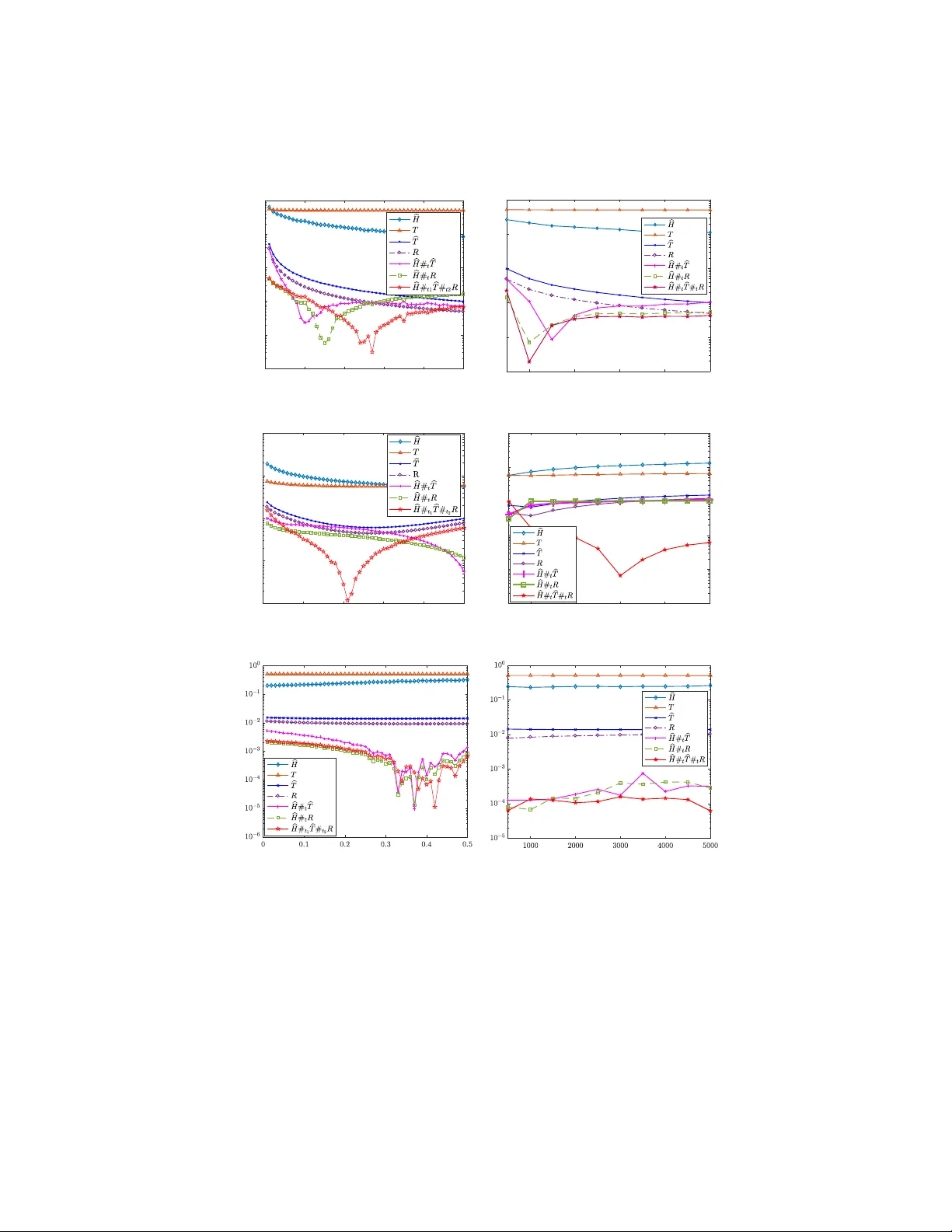
F ast computation of v on Neumann en trop y for large-scale graphs via quadratic appro ximations Ha young Choi ∗ , Jinglian He , Hang Hu , Y uanming Shi Scho ol of Information Scienc e and T echnolo gy, ShanghaiT e ch University Abstract The von Neumann graph en tropy (VNGE) can b e used as a measure of graph complexit y , which can b e the measure of information div ergence and distance b et ween graphs. Ho wev er, computing VNGE is extensiv ely demanding for a large-scale graph. W e propose nov el quadratic approximations for fast computing VNGE. V arious inequalities for error b et ween the quadratic appro ximations and the exact VNGE are found. Our metho ds reduce the cubic complexity of VNGE to linear complexity . Computational simulations on random graph mo dels and v arious real netw ork datasets demonstrate sup erior p erformance. Keywor ds: V on Neumann entrop y, V on Neumann graph entrop y, graph dissimilarit y, densit y matrix 2010 MSC: 05C12, 05C50, 05C80, 05C90, 81P45, 81P68 1. In tro duction Graph is one of the most common represe n tations of complex data. It has the sophisticated capability of representing and summarizing irregular structural features. T o da y , graph-based learning has b ecome an emerging and promising metho d with n umerous applications in many v arious fields. With the increasing quan tity of graph data, it is crucial to find a wa y to manage them effectiv ely . Graph similarity as a typical wa y of presenting the relationship b et ween graphs ha ve b een v astly applied [ 28 , 11 , 7 , 1 , 10 ]. F or example, Sadreazami et al. prop osed an in trusion detection metho dology based on learning graph similarity with a graph Laplacian matrix [ 25 ]; also, Y anardag and Vishw anathan gav e a general framew ork to smooth graph kernels based on graph similarity [ 29 ]. Ho wev er, all the ab o v e approaches relied on presumed mo dels, and th us limited their abilit y of being applied on comprehending the general concept of div ergences and distances b et ween graphs. ∗ Corresponding author. Email addr esses: hchoi@shanghaitech.edu.cn (Hay oung Choi), hejl1@shanghaitech.edu.cn (Jinglian He), huhang@shanghaitech.edu.cn (Hang Hu), shiym@shanghaitech.edu.cn (Y uanming Shi) Pr eprint submitte d to Elsevier July 23, 2019 Mean while, graph entrop y [ 3 ] which is a mo del-free approach, has b een activ ely used as a wa y to quan tify the structural complexity of a graph. By regarding the eigenv alues of the normalized combinatorial Laplacian of a graph as a probability distribution, we can obtain its Shannon en tropy . By giving the density matrix of a graph, which is the representation of a graph in a quan tum mechanical state, w e can calculate its von Neumann en tropy for a graph [ 4 ]. Bai et al. prop osed an algorithm to solve the depth-based complexit y c haracterization of the graph using von Neumann entrop y [ 5 ]. Liu et al. ga ve a metho d of detecting a bifurcation net work even t based on v on Neumann entrop y [ 20 ]. Other applications include graph clustering [ 6 ], netw ork analysis [ 30 ], and structural reduction of multiplex net works [ 12 ]. Ho w ever, the c ost of computing the exact v alue is highly exp ensiv e for a large-scale graph. 1.1. V on Neumann entr opy The von Neumann entrop y , which was introduced b y John von Neumann, is the extension of classical entrop y concepts to the field of quantum mec hanics [ 17 ]. He introduced the notion of the density matrix, which facilitated the extension of the to ols of classical statistical me c hanics to the quantum domain in order to dev elop a theory of quantum measuremen ts. Denote the trace of a square matrix A as tr A . A density matrix is a Hermitian p ositiv e semidefinite with unite trace. The density matrix ρ is a matrix that describ es the statistical state of a system in quan tum mec hanics. The density matrix is especially useful for dealing with mixed states, whic h consist of a statistical ensem ble of several differen t quan tum systems. The von Neumann entr opy of a density matrix ρ , denoted by H ( ρ ), is defined as H ( ρ ) = − tr( ρ ln ρ ) = − n X i =1 λ i ln λ i , where λ 1 , . . . , λ n are eigen v alues of ρ . It is conv entional to define 0 ln 0 = 0. This definition is a prop er extension of b oth the Gibbs entrop y and the Shannon en tropy to the quan tum case. 1.2. V on Neumann gr aph entr opy In this article we consider only undirected simple graphs with non-negative edge weigh ts. Let G = ( V , E , W ) denote a graph with the set of vertices V and the set of edges E , and the weigh t matrix W . The c ombinatorial gr aph L aplacian matrix of G is defined as L ( G ) = S − W , where S is a diagonal matrix and its diagonal entry s i = P n j =1 W ij . The density matrix of a graph G is defined as ρ G = 1 tr ( L ( G )) L ( G ) , where 1 tr ( L ( G )) is a trace normalization factor. Note that ρ G is a pos itiv e semidefinite matrix with unite trace. The von Neumann entr opy for a graph G , denoted by H ( G ), is defined as H ( G ) := H ( ρ G ) , 2 where ρ G is the density matrix of G . It is also called von Neumann gr aph entr opy (VNGE). Computing von Neumann graph entrop y requires the entire eigensp ectrum { λ i } n i =1 of ρ G . This calculation can b e done with time complexity O ( n 3 ) [ 16 ], making it computationally impractical for large-scale graphs. F or example, the von Ne umann graph entrop y hav e b een prov ed to b e an feasible approach in the computation of Jensen-Shannon distance b etw een any t wo graphs from a graph sequence [ 12 ]. Ho wev er, in the pro cess of machine learning and data mining tasks, a sequence of large-scale graphs will b e inv olved. Therefore, it is of great significance to find an efficient metho d to compute the von Neumann entrop y of large-scale graphs faster than the previous O ( n 3 ) approac h. More details ab out the application of Jensen-Shannon distance will b e sho wn in Section 4 . T o tackle this challenge ab out com putational inefficiency , Chen et al. [ 9 ] prop osed a fast algorithm for computing von Neumann graph en tropy , which uses a quadratic p olynomial to approximate the term − λ i ln λ i rather than extracting the eigensp ectrum. It was sho wn that the prop osed appro ximation is more efficient than the exact algorithm based on the singular v alue decomp osition. Although it is true that our work w as inspired by [ 9 ], the prior work needs to calculate the largest eigenv alue for the appro ximation. Our prop osed metho ds do es not need the largest eigenv alue to appro ximate VNGE, so the computational cost is slightly b etter than the prior w ork. Moreo ver, our prop osed metho ds hav e sup erior p erformances in random graphs as well as real datasets with linear complexity . 2. Quadratic Appro ximations F or a Hermitian matrix A ∈ C n × n it is true that tr f ( A ) = P i f ( λ i ) where { λ i } n i =1 is the eigenspectrum of A . Since H ( ρ ) = − tr ( ρ ln ρ ), one natural approac h to approximate the von Neumann entrop y of a density matrix is to use a T a ylor series expansion to appro ximate the logarithm of a matrix. It is required to calculate tr ( ρ j ) , j ≤ N for some p ositive integer N . Indeed, ln ( I n − A ) = − P ∞ j =1 A j /j for a Hermitian matrix A whose eigenv alues are all in the in terv al ( − 1 , 1). Assuming that all eigen v alues of a density matrix ρ are nonzeros, we ha ve H ( ρ ) = − ln λ max + N X j =1 1 j tr  ρ ( I n − ( λ max ) − 1 ρ ) j  , where λ max is the maximum eigenv alue of ρ . W e refer to [ 19 ] for more details. Ho wev er, the computational complexity is O ( n 3 ), so it is impractical as n gro ws. In this article, w e propose quadratic approximations to approximate the v on Neumann entrop y for large-scale graphs. It is noted that only tr ( ρ 2 ) is needed to compute them. W e consider v arious quadratic p olynomials f app ( x ) = c 2 x 2 + c 1 x + c 0 to approximate f ( x ) = − x ln x on (0 , 1] ( f (0) = 0). Then H ( ρ ) = tr ( f ( ρ )) ≈ tr ( f app ( ρ )) = P n i =1 f app ( λ i ) = c 2 tr ( ρ 2 ) + c 1 + c 0 n. Suc h appro ximations are required to b e considered on the only v alues in [0 , 1] such that their sum is 1, which are eigenv alues of a given densit y matrix. 3 Recall that tr ( ρ 2 ) is called purity of ρ in quantum information theory . The purit y gives information on ho w muc h a state is mixed. F or a given graph G , the purity of ρ G can b e computed efficiently due to the sparsity of the ρ G as follo ws. Lemma 1. F or a gr aph G = ( V , E , W ) ∈ G , tr ( ρ 2 G ) = 1 (tr ( L )) 2 X i ∈ V S 2 ii + 2 X ( i,j ) ∈ E L 2 ij ! . Pr o of. Since L , ρ G are symmetric, it follows that tr ( ρ 2 G ) = || ρ G || 2 F = 1 (tr L ) 2 || L || 2 F = 1 (tr L ) 2 X 1 ≤ i,j ≤ n L 2 ij = 1 (tr L ) 2 X 1 ≤ i ≤ n L 2 ii + 2 X 1 ≤ i 0. Th us, − λ max ln λ max − (1 − λ max ) ln (1 − λ max ) ≥ − λ max ( λ max − 1) − (1 − λ max )( − λ max ) = 2 λ max (1 − λ max ) . (2) Since tr ( ρ 2 ) ≤ λ 2 1 + ( λ 2 + · · · + λ n ) 2 , clearly tr ( ρ 2 ) ≤ λ 2 1 + (1 − λ 1 ) 2 . F or a pro of of the first inequalit y , see [ 18 ]. (3) By Prop osition 1 (2), clearly 1 /n ≤ tr ( ρ 2 ) ≤ 1. Since f ( x ) = − x ln x is conca ve on [0 , 1], b y Jensen’s inequality , it follows that f (tr ( ρ 2 )) = f n X i =1 λ 2 i ! ≥ n X i =1 λ i f ( λ i ) = n X i =1 − λ 2 i ln λ i . This article considers the following quadratic appro ximations for von Neu- mann en tropy: (i) FINGER- b H ; (ii) T a ylor- T ; (iii) Mo dified T a ylor- b T ; (iv) Radial Pro jection- R . Note that they all can b e computed by the purity of density matrix of a graph. Additionally (i) and (iii) need to compute the maxim um eigen v alue as w ell. 2.1. FINGER- b H Chen et al.[ 9 ] proposed a fast incr emental von Neumann gr aph entr opy (FINGER) to reduce the cubic complexity of von Neumann graph en tropy to linear complexity . They considered the follo wing quadratic p olynomial to appro ximate f ( x ) = − x ln x (see Fig. 1 ). q ( x ) = − (ln λ max ) x (1 − x ) on [0 , 1] . (1) 5 Then FINGER, denoted by b H , is defined as b H ( G ) := n X i =1 q ( λ i ) = − (ln λ max )(1 − tr( ρ 2 G )) , where λ 1 , . . . , λ n are the eigen v alues of ρ G . Note that since all eigenv alues are smaller than or equal to the maximum eigen v alue, it is b etter to deal with the functions f and q on the interv al [0 , λ max ] instead of [0 , 1]. Now let us sho w that the approximation FINGER is alwa ys smaller than the exact v on Neumann entrop y . Lemma 2. The fol lowing ar e true. (1) f − q is c onc ave on [0 , λ max ] . (2) f ( x ) − q ( x ) ≥ λ max f ( x ) on [0 , λ max ] . Pr o of. It is trivial for λ max = 1. Supp ose that λ max 6 = 1. (1) Note that f ( x ) < 1 /e < 1 / 2 on all 0 ≤ x ≤ 1. So, − λ max ln λ max < 1 / 2. Then λ max < 1 − 2 ln λ max , implying, − 1 − 2 x ln λ max < 0 for all 0 ≤ x ≤ λ max . Th us, ( f − q ) 00 ( x ) = − 1 − 2 x ln λ max x < 0 . (2) When x = 0 or x = λ max , it is trivial. Since (1 − λ max ) f ( x ) − q ( x ) = x (( λ max − 1) ln x + ( ln λ max )(1 − x )), it suffices to sho w φ ( x ) = ( λ max − 1) ln x + ln λ max (1 − x ) > 0 for all 0 < x < λ max . By observing the tangen t line at x = 1 for y = x ln x , it is easy to chec k that λ max − 1 < λ max ln λ max . Then λ max − 1 ln λ max > λ max . Th us, φ 0 ( x ) = λ max − 1 x − ln λ max < 0 for all 0 < x < λ max . Since φ ( λ max ) = 0 and φ 0 ( x ) < 0 for all 0 < x < λ max , it follows that φ ( x ) > 0 for all 0 < x < λ max . Theorem 1. F or any density matrix ρ , it holds that (1) b H ( λ 1 , . . . , λ n ) ≥ b H ( λ max , 1 − λ max ) . (2) H ( ρ ) ≥ b H ( ρ ) The e quality holds if and only if λ max = 1 . (3) H ( ρ ) − b H ( ρ ) ≥ λ max H ( ρ ) . Pr o of. (1) Let φ ( x ) = x (1 − x ). Then it is easy to chec k that φ ( t 1 ) + φ ( t 2 ) − φ ( t 1 + t 2 ) ≥ 0 for all t 1 , t 2 ≥ 0. Thus, q ( t 1 + t 2 ) ≤ q ( t 1 ) + q ( t 2 ). By induction, it holds that q ( t 1 + · · · + t n ) ≤ q ( t 1 ) + · · · q ( t n ) , 6 for all t i ≥ 0, i = 1 , . . . , n . Then it follows that b H ( λ 1 , . . . , λ n ) = n X i =1 q ( λ i ) = q ( λ 1 ) + n X i =2 q ( λ i ) ≤ q ( λ 1 ) + q  n X i =2 λ i  = q ( λ 1 ) + q (1 − λ 1 ) , where λ n ≤ · · · ≤ λ 1 are sp ectrum of ρ . (2) Let λ b e an eigenv alue of ρ . Since λ ≤ λ max , it follo ws that f ( λ ) − q ( λ ) = − λ ln λ + (ln λ max ) λ (1 − λ ) ≥ − λ ln λ + (ln λ ) λ (1 − λ ) = − λ 2 ln λ ≥ 0 . Note that 0 = λ n = · · · = λ 2 and λ 1 = 1 if and only if λ 2 i ln λ i = 0 for all 1 ≤ i ≤ n . (3) By Lemma 2 (2) we can find the error b ound for FINGER. F or more information ab out FINGER, see [ 9 ]. 2.2. T aylor- T Since the sum of all eigenv alues of densit y matrix is 1, the av erage of them is 1 n . As n gets bigger, the av erage gets closer to 0. Thus, for a large-scale n × n densit y matrix, man y of its eigenv alues must b e on [0 , 1 n ]. So, it is reasonable to use T a ylor series for f at x = 1 n instead of x = 0. In fact, since f 0 (0) do es not exist, there do es not exist T a ylor series for f at x = 0. Lemma 3. L et λ max b e the maximum eigenvalue of a density matrix ρ . Then, 1 n ≤ λ max ≤ 1 . Esp e cial ly, λ max = 1 if and only if H ( ρ ) = 0 . Also it is true that λ max = 1 n if and only if H ( ρ ) = ln( n ) . Pr o of. Since tr ρ = 1, if λ max = 1 then all eigenv alues are 0 except λ max . It is kno wn that H ( ρ ) ≤ ln( n ) and the equality holds when λ i = 1 n for all i . W e can prop ose the quadratic T aylor appro ximation for f at x = 1 n as follows. q ( x ) = f  1 n  + f 0  1 n  x − 1 n  + f 00 ( 1 n ) 2!  x − 1 n  2 = − n 2 x 2 + (ln n ) x − 1 2 n . 7 0 0.1 0.2 0.3 0.4 0.5 0.6 0.7 0.8 0.9 1 0 0.1 0.2 0.3 0.4 0.5 0.6 y = -xln(x) max = 0.1 max = 0.2 max = 0.4 max = 0.6 max = 0.8 max (1/n,f(1/n)) Figure 2: Mo dified T a ylor- b T : graphs of the quadratic function in ( 2 ) with differen t λ max are shown. Using such appro ximation, T a ylor, denoted b y T , is defined as T ( G ) = − n 2 tr( ρ 2 G ) + ln n − 1 2 . As Fig. 2 shows, the function q is very similar to the function f near x = 1 n . Ho wev er, as the maxim um eigen v alue gets closer to 1, the error b ecomes v ery large. Note that f ( λ max ) − q ( λ max ) = − λ max ln λ max + n 2 λ 2 max − ( ln n ) λ max − 1 2 n − → ∞ as n − → ∞ for λ max ≈ 1. Alternativ ely , this approximation needs to be mo dified. W e use the information ab out λ max in order to reduce the error. W e assume that the eigenv alues concentrate around the mean 1 /n . Remark that this w ould b e in general true for small-w orld or relativ ely small-world graphs, but for example in planar graphs or graphs represen ting a low dimensional manifold where W eyl’s law holds this would not b e true. In particular for planar geometry or 2 D manifolds the smallest eigen v alues would grow linearly , and this rate would most likely hold well around 1 /n . 2.3. Mo difie d T aylor- b T Consider the quadratic appro ximation, q , to approximate f ( x ) = − x ln x suc h that it holds q  1 n  = f  1 n  , q 0  1 n  = f 0  1 n  , q ( λ max ) = f ( λ max ) , assuming that λ max 6 = 1 n , we ha ve q ( x ) = σ x 2 +  ln n − 1 − 2 σ n  x + σ + n n 2 , (2) where σ = − nλ max ln ( nλ max ) + nλ max − 1 n ( λ max − 1 n ) 2 . 8 Using such approximation, the Mo dified T a ylor, denoted by b T , is defined as b T ( G ) = σ  tr( ρ 2 G ) − 1 n  + ln n. Lemma 4. The fol lowing ar e true. (1) q is c onc ave on [0 , λ max ] . (2) 1 n ≤ − 1 2 σ ≤ λ max . Pr o of. (1) Since q is a quadratic p olynomial in x , it suffices to show σ < 0. Let φ ( t ) = − t ln t + t − 1. Since φ (1) = 0 and φ 0 ( t ) < 0 for all t > 1, it is true that φ ( t ) < 0 for all t > 1. By Lemma 3 , nλ max > 1, so φ ( nλ max ) = − nλ max ln ( nλ max ) + nλ max − 1 < 0. (2) Let t = nλ max . By Lemma 3 , t > 1. Since 1 − 2 σ − 1 n = 1 n ( t − 1) 2 2( t ln t − t + 1) − 1 ! , It suffices only if we show ( t − 1) 2 > 2( t ln t − t + 1). Recall that t ln t − t + 1 > 0 for all t > 1. Let φ ( t ) = t 2 − 2 t ln t − 1. Since ln t < t − 1 for all t , φ 0 ( t ) = 2 t − 2 ln t − 2 = 2(( t − 1) − ln t ) > 0 for all t ≥ 1. F rom the fact φ (1) = 0, clearly , φ ( t ) > 0 for all t > 1. So, 1 n ≤ − 1 2 σ . T aking t = nλ max , w e ha ve λ max − 1 − 2 σ = t n − ( t − 1) 2 2 n ( t ln t − t + 1) = 2 t ( t ln t − t + 1) − ( t − 1) 2 2 n ( t ln t − t + 1) > 0 . Theorem 2. F or any density matrix ρ , it holds that b T ( ρ ) ≥ H ( ρ ) . Pr o of. Let h ( x ) = q ( x ) − f ( x ). Clearly , h (1 /n ) = h ( λ max ) = 0 and h 0 (1 /n ) = 0. W e sho w that h ( x ) ≥ 0 for three different in terv als: (i) [0 , 1 n ], (ii) [ 1 n , − 1 2 σ ], and (iii) [ − 1 2 σ , λ max ]. (i) Since h 00 = 2 σ + 1 x , Lemma 4 (2) implies that h is conv ex on [0 , − 1 2 σ ]. Since h (1 /n ) = h 0 (1 /n ) = 0, h ( x ) ≥ 0 on [0 , 1 n ]. (ii) In the similar w ay , it holds that h ( x ) ≥ 0 on [ 1 n , − 1 2 σ ]. (iii) Since h is concav e on [ − 1 2 σ , λ max ], b y the definition of concavit y , it follows that h  − 1 2 σ t + λ max (1 − t )  ≥ h  − 1 2 σ  t + h ( λ max )(1 − t ) ≥ 0 for all 0 ≤ t ≤ 1. The last inequality holds from the fact that h ( − 1 2 σ ) ≥ 0 and h ( λ max ) = 0. Th us, h ( x ) ≥ 0 on [ − 1 2 σ , λ max ]. Therefore, by (i), (ii), (iii) it holds that h ( x ) ≥ 0 on [0 , λ max ]. 9 1 0.8 0.6 1 0.9 0.8 0.7 0.4 0.6 0.5 0.4 0.3 0.2 0.1 0 1 0.2 0 0.5 0 0.1 0.2 0.3 0.4 0.5 0.6 0.7 0.8 0.9 1 Figure 3: The Shannon entrop y at each point ( λ 1 , λ 2 , λ 3 ) ∈ ∆ 3 with differen t color lev els. 2.4. R adial Pr oje ction- R W e denote the simplex of p ositiv e probability as ∆ n , i.e., ∆ n := n ( λ 1 , λ 2 , . . . , λ n )    n X i =1 λ i = 1 , λ i ≥ 0 o . Also w e denote E := (1 /n, . . . , 1 /n ). Clearly , E ∈ ∆ n . The Shannon entr opy of Λ ∈ ∆ n is defined as S (Λ) = − P n i =1 λ i ln λ i . It is well-kno wn that it holds S (Λ) ≤ ln n , with equality if Λ = E . That is, E is the only point where the en tropy is maximum. As Fig. 3 is sho wn, the simplex of p ositive probability ∆ 3 can be geometrically presen ted as a part of plane in R 3 . The color stands for the v alue of Shannon en tropy at each p oin t. One can see that as Λ ∈ ∆ 3 gets closer to E , the entrop y gets bigger and bigger. Our main observ ation is that if tw o p oin ts on ∆ 3 ha ve same (Euclidean) distances from E , then their purity are same. In general it holds for an y n . Lemma 5. L et Λ = ( λ 1 , λ 2 , . . . , λ n ) ∈ ∆ n . Then the fol lowing ar e true. (1) ||E − Λ || 2 2 = P n i =1 λ 2 i − 1 n . (2) hE , E − Λ i = 0 . ( h· , ·i is the usual inner pr o duct.) Pr o of. It is easy to chec k that ||E − Λ || 2 2 = n X i =1  λ i − 1 n  2 = n X i =1 λ 2 i − 1 n . 10 Theorem 3. L et ρ and ˜ ρ b e n × n density matric es. Then || ρ − 1 /n I || F = || e ρ − 1 /n I || F if and only if their purity ar e identic al. Pr o of. Note that || ρ − 1 /n I || F = || e ρ − 1 /n I || F if and only if ||E − Λ || 2 = ||E − e Λ || 2 , where λ 1 , λ 2 , . . . , λ n and ˜ λ 1 , ˜ λ 2 , . . . , ˜ λ n are eigenv alues of ρ and e ρ , resp ectiv ely . It is true from Lemma 5 . Lemma 5 states that tw o p oints on ∆ n ha ve the same distance from E if and only if the distances from the origin are identical. Then w e can find ˜ Λ ∈ ∆ n whose entrop y can b e computed muc h easily suc h that ||E − Λ || 2 = ||E − e Λ || 2 . There are infinitely many directions from E to find ˜ Λ ∈ ∆ n . Among them we pic k w = ( c, 1 − c n − 1 , . . . , 1 − c n − 1 ) ∈ ∆ n with c = λ max . W e consider the line segment ` ( t ) = ( w − E ) t + E , 0 ≤ t ≤ 1, i.e., ` ( t ) =  1 − t n + tc, 1 − t n + t (1 − c ) n − 1 , . . . , 1 − t n + t (1 − c ) n − 1  . Since ∆ n is conv ex, ` ( t ) ∈ ∆ n for all 0 ≤ t ≤ 1. F or each 0 ≤ t ≤ 1, we hav e S ( ` ( t )) = −  1 − t n + tc  ln  1 − t n + tc  − ( n − 1)  1 − t n + t (1 − c ) n − 1  ln  1 − t n + t (1 − c ) n − 1  . Lemma 5 implies that ||E − ` ( t ) || 2 2 = t 2 || w − E || 2 2 = ( cn − 1) 2 n ( n − 1) t 2 . W e solv e the following equation for 0 ≤ t ≤ 1: ||E − Λ || 2 = ||E − ` ( t ) || 2 . Then the solution, say t 0 , is t 0 = p n ( n − 1) cn − 1 v u u t n X i =1 λ 2 i − 1 n . Since ||E − Λ || 2 = ||E − ` ( t 0 ) || 2 , we ha ve that S (Λ) ≈ S ( ` ( t 0 )) = −  1 − t 0 n + t 0 c  ln  1 − t 0 n + t 0 c  − ( n − 1)  1 − t 0 n + t 0 (1 − c ) n − 1  ln  1 − t 0 n + t 0 (1 − c ) n − 1  . 11 In fact, putting t 0 in to the right side the constant c can b e cancelled. Th us, this appro ximation do es not need the maximum eigen v alue. No w we prop ose the quadratic approximation for the von Neumann graph en tropy , called Radial Pro jection, denoted by R , is defined as R ( G ) = −  r n − 1 n κ G + 1 n  ln  r n − 1 n κ G + 1 n  − ( n − 1)  − 1 p ( n − 1) n κ G + 1 n  ln  − 1 p ( n − 1) n κ G + 1 n  , (3) where κ G = [tr( ρ 2 G ) − 1 n ] 1 / 2 . 2.5. Weighte d me an Denote the w eighted mean of a, b ∈ R as a # t b . That is, a # t b = ta + (1 − t ) b. In a similar w ay w e consider b H ( ρ )# t b T ( ρ ) and b H ( ρ )# t R ( ρ ). By Theorem 1 (2), it is shown that FINGER- b H is alwa ys smaller than the exact von Neumann en tropy . On the other hand, by Theorem 2 Modified T a ylor- b T is alw a ys greater than the exact v on Neumann entrop y . Ev en though it is not prov ed mathematically , Fig. 3 , 6 , 7 show that Radial pro jection- R are greater than the exact von Neumann entrop y . The w eighted mean of them can b e computed to impro ve the appro ximations. W e solve a optimization problem to find optimal t ∗ . F or example, consider b H # t b T . Giv en large quantit y of real data sets, the approximation of von Neumann en tropy using b H and b T w ere calculated as the input v alues x ( i ) b T and x ( i ) b H while the actual von Neumann entrop y v alue were also calculated as output v alues y ( i ) for i = 1 , . . . , N ( N is the num b er of data sets). Then the optimization problem is given as follows: t ∗ = arg min 0 ≤ t ≤ 1 J ( t ) , where the cost function is J ( t ) = 1 N N X i =1  tx ( i ) b H + (1 − t ) x ( i ) b T − y ( i )  2 . W e use the gradient descen t metho d to find optimal t ∗ . Initially , t 0 = 1 2 is given. In each step of gradien t descen t, t j is up dated with the function: t j = t j − 1 − αJ 0 ( t j − 1 ) , where j denotes iteration times, and α is the step size, whic h is set to b e 10 − 6 . One may wander if such “real data sets” are indep endent of the test netw orks emplo yed in the numerical exp eriments. On the one hand they should, in order to av oid a circular argument; on the other hand, to b e effectiv e suc h “training” should someho w extract the generalities of a class of graphs. In order to eliminate 12 o verfitting, w e separated our datasets into tw o parts, the training datasets and the test datasets. After w e got the optimal weigh ts t ∗ using the pro cess stated ab o ve with training datasets, we calculate the appro ximate v alue V 1 of the test datasets. Then we use test datasets to find the optimal t ∗ test and calculate the appro ximate v alue V 2 using t ∗ test , the av erage difference b et ween V 1 and V 2 are lo wer than 0 . 02, which is acceptable. Ho wev er, it is still questionable to show mathematically that t ∗ is optimal. Using the optimal v alues t ∗ solv ed by the gradient descent metho d, we call b H # 0 . 3824 b T and b H # 0 . 2794 R as Impr ove d Mo difie d T aylor and Impr ove d R adial Pr oje ction , respectively . As anonymous referee suggested, we also consider ω 1 b H + ω 2 T + ω 3 b T + ω 4 R + β , where ω i are weigh ts suc h that 0 ≤ ω i ≤ 1 and ω 1 + · · · + ω 4 = 1, and β ∈ R is a constant shift. In a similar wa y , the optimal w eights can b e found. It is shown that 0 . 2299 b H + 0 . 3099 b T + 0 . 4602 R − 0 . 0073 has sup erior p erformances for real datasets. W e call this as Mixe d Quadr atic appr oximiation . 3. Exp erimen ts 3.1. R andom gr aphs In this section results from v arious exp eriments with data sets are provided. All exp eriments w ere conducted b y MA TLAB R2016 on a 16-core machine with 128GB RAM. Three random graph mo dels are considered: (i) the Erd˝ os-R ´ en yi (ER) mo del [ 14 , 15 ] - the ER mo del represen ts tw o closely related models that were introduced indep enden tly and sim ultaneously . Here w e use the ER model which w as prop osed b y Gilb ert [ 15 ]. G ( n, p ) is denoted as a mo del with n no des, and each pair of no des w ere linked indep enden tly with probabilit y 0 ≤ p ≤ 1; (ii) the Barab´ asi- Alb ert (BA) model [ 2 ] - the BA mo del is a sp ecial case of the Price’s model. It can generate scale-free graphs in whic h the degree distribution of the graph follo ws the pow er law distribution; and (iii) the W atts-Strogatz (WS) mo del [ 27 ] - the WS mo del generates graphs with small w orld prop erties, given a net work with N no des and the mean degree K, initially no des are linked as a regular ring where each no de is connected to K/ 2 no des in eac h side, then rewire the edges with probability 0 ≤ p ≤ 1. The appro ximation error is defined as | E xact − Appr oximation | . The results are av eraged ov er 50 random trials. The simulations demonstrate that Impro ved Mo dified T a ylor and Improv ed Radial Pro jection hav e best p erformances. Ho wev er, they are required to compute the maximum eigen v alue. Thus, the computational cost is sligh tly higher than Radial Pro jection whic h does not need to compute the maximum eigenv alue. Th us considering the time cost, Radial Pro jection is the sup erior metho d. Theorem 1 (2) states that FINGER- b H is alwa ys smaller than the exact von Neumann en tropy . On the other hand, b y Theorem 3 Mo dified T aylor- b T is alw ays greater than than the exact von Neumann en tropy . Additionally , Theorem 3 sho ws that FINGER b H ( ρ ) is b ounded ab o ve by (1 − λ max ) H ( ρ ). That is, the FINGER is alwa ys under-estimated whose error is bigger than λ max H ( ρ ). In 13 0 200 400 600 800 1000 Average degree 10 -5 10 -4 10 -3 10 -2 10 -1 10 0 Error (a) ER a verage degree 1000 2000 3000 4000 5000 Number of nodes 10 -5 10 -4 10 -3 10 -2 10 -1 10 0 Error (b) ER no des 0 200 400 600 800 1000 Average degree 10 -3 10 -2 10 -1 10 0 10 1 Error (c) BA a verage degree 1000 2000 3000 4000 5000 Number of nodes 10 -4 10 -3 10 -2 10 -1 10 0 10 1 Error (d) BA no des Edge rewiring probability Error (e) WS a verage degree Number of nodes Error (f ) WS no des Figure 4: Error of the approximations for three random models: (i) Erd˝ os-R´ enyi (ER) mo del; (ii) Barab´ asi-Albert (BA) mo del; (iii) W atts-Strogatz (WS) model. a similar w ay , b T is alw ays ov er-estimated. Although we could not find the minim um error mathematically , the simulation results for lots of dataset sho w that the minim um error is strictly bigger than 0. 14 7.4 7.42 7.44 7.46 7.48 7.59835 7.5984 7.59845 7.5985 VNGE 7.100902218 7.10090222 7.59835 7.5984 7.59845 7.5985 VNGE 7.60090278 7.6009028 7.60090282 7.59835 7.5984 7.59845 7.5985 VNGE 7.5996 7.59962 7.59964 7.59966 7.59835 7.5984 7.59845 7.5985 VNGE 7.15 7.2 7.25 7.3 7.5858 7.586 7.5862 7.5864 7.5866 7.5868 VNGE 7.10089701 7.100897011 7.100897012 7.5858 7.586 7.5862 7.5864 7.5866 7.5868 VNGE 7.6009065 7.600907 7.6009075 7.600908 7.5858 7.586 7.5862 7.5864 7.5866 7.5868 VNGE 7.5954 7.5955 7.5956 7.5858 7.586 7.5862 7.5864 7.5866 7.5868 VNGE 6.78 6.79 6.8 6.81 6.82 7.5345 7.535 7.5355 VNGE 7.1009023362 7.10090233624 7.5345 7.535 7.5355 VNGE 7.60090248 7.600902482 7.600902484 7.5345 7.535 7.5355 VNGE 7.5829 7.583 7.5831 7.5345 7.535 7.5355 VNGE Figure 5: Entropies correlations on the ER model (top), BA model (middle) and WS mo del (bottom). In order to further analyze the p erformance of our prop osed algorithms, w e p erform a correlation study b etw een the exact von Neumann en tropy and corresp onding approximate v alue returned b y four appro ximation algorithms on three different random graph mo del. More sp ecifically , for each mo del, we generate 50 graphs. Fig. 5 shows the results of the correlation analysis. It is sho wn that there exists a strong correlation b etw een the exact VNGE and its appro ximation obtained b y Radial Pro jection on all random graphs. W e then observ e that correlation betw een exact VNGE and its approximation got b y T a ylor is strong on BA and WS mo del, but b ecomes muc h weak er on ER mo del. The reader is referred to [ 21 ] for a recent analysis of FINGER approximation for graph Laplacians. 3.2. R e al-world datasets The real-world datasets in v arious fields are considered [ 24 , 23 , 22 ]. W e use 137 differen t num b er of unw eigh ted netw orks and 48 differen t num b er of weigh ted net works in different fields for simulations. The detailed information ab out datasets on Fig. 6 and Fig. 7 can be found at https://github.com/Hang14/RDJ . Fig. 6 and Fig. 7 show the scatter p oin ts of the v on Neumann en tropy (y- axis) versus the quadratic appro ximations (x-axis) for b oth the unw eighted and weigh ted real-w orld datasets. It demonstrates that Modified T a ylor and Radial Pro jection hav e b etter p erformances than FINGER. Mixed Quadratic appro ximation sho ws the b est p erformance. 3.3. Time c omp arison Recall that computing von Neumann graph entrop y requires O ( n 3 ) computa- tional complexity . In order to accelerate its computation, we use the quadratic 15 0 1 2 3 4 5 6 7 8 9 10 0 1 2 3 4 5 6 7 8 9 10 0 1 2 3 4 5 6 7 8 9 10 0 1 2 3 4 5 6 7 8 9 10 0 1 2 3 4 5 6 7 8 9 10 0 1 2 3 4 5 6 7 8 9 10 0 1 2 3 4 5 6 7 8 9 10 0 1 2 3 4 5 6 7 8 9 0 1 2 3 4 5 6 7 8 9 10 0 1 2 3 4 5 6 7 8 9 0 1 2 3 4 5 6 7 8 9 10 0 1 2 3 4 5 6 7 8 9 Brain Collaboration Protein BHOSLIB Power Road Facebook Web Communication Figure 6: Exact entrop y v ersus approximate entrop y for the unw eighted real datasets. appro ximations for the function f ( x ) = − x ln x . Then eac h appro ximation can b e computed by the purity of the density matrix for a given graph. Lemma 1 sho ws that computing the purity requires O ( n + m ) computational complexit y , where | V | = n and | E | = m . How ev er, FINGER and Mo dified T aylor addition- ally need to compute the maximum eigenv alue whose time complexity is O ( n 2 ) [ 16 ]. On the other hand, Radial pro jection shows the b est performance with no maxim um eigen v alue. When the original graph is a complete graph then | E | = n 2 whic h is also the upp er b ound of | E | . Ho wev er, in real life sce nario, complete graph is rare, instead, sparse graph are more commonly seen, therefore, the time complexit y can remain in a rather linear form. 4. Applications One ma jor application of von Neumann graph entrop y is the computation of Jensen-Shannon distance(JSdist) b et ween any tw o graphs from a graph sequence [ 12 ]. Given a graph sequence G , the Jensen-Shannon distance of any tw o graphs G = ( V , E , W ) ∈ G and G 0 = ( V , E 0 , W 0 ) ∈ G is defined as JSdist( G, G 0 ) = r H ( G ) − 1 2 [ H ( G ) + H ( G 0 )] , where G = ( V , E , W ) = G ⊕ G 0 2 is the av eraged graph of G and G 0 suc h that W = W + W 0 2 . The Jensen-Shannon distance has been prov ed to be a v alid 16 0 1 2 3 4 5 6 7 8 9 10 0 1 2 3 4 5 6 7 8 9 10 0 1 2 3 4 5 6 7 8 9 10 0 1 2 3 4 5 6 7 8 9 10 0 1 2 3 4 5 6 7 8 9 10 0 1 2 3 4 5 6 7 8 9 10 0 1 2 3 4 5 6 7 8 9 10 0 1 2 3 4 5 6 7 8 9 0 1 2 3 4 5 6 7 8 9 10 0 1 2 3 4 5 6 7 8 9 0 1 2 3 4 5 6 7 8 9 10 0 1 2 3 4 5 6 7 8 9 Biology Collaboration Ecology Economy Facebook Retweet Power Figure 7: Exact entrop y v ersus approximate entrop y for the weigh ted real datasets. distance metric in [ 13 , 8 ]. The Jensen-Shannon distance hav e b een applied into many fields including net work analysis [ 12 ] and machine learning [ 26 ]. Esp ecially , it can b e used in anomaly detection and bifurcation detection [ 20 ]. [ 9 ] demonstrated the v alidation of using FINGER for computing VNGE. Comparing to the state-of-art graph similarit y metho ds, FINGER yields sup erior and robust performance for anomaly detection in evolving Wikip edia net works and router communication net works, as well as bifurcation analysis in dynamic genomic netw orks. Note that the sim ulations sho w that our prop osed metho ds show b etter p erformance than FINGER. 5. Final remarks W e prop osed quadratic appro ximations for efficiently estimating the v on Neumann entrop y of large-scale graphs. It reduces the computation of VNGE from cubic complexity to linear complexit y for a given graph. W e finally close with some op en problems arisen during our study . (1) In Theorem 2 , the mo dified T a ylor- b T is alwa ys bigger than VNGE. Ho wev er, It is still op en if there exists any error b ound for b T whic h is same as or similar to Theorem 1 (3). 17 (2) The sim ulations show that Radial pro jection- R ha ve superior p erformances without any information ab out the maximum eigenv alue. Ho w ever, it is questionable if there exists some error b ound b et ween v on Neumann en tropy and Radial pro jection. (3) Fig. 4 shows that the error for weigh ted means hav e interesting b eha viors. F urther analysis is needed with different class of graphs. It remains for future work. Ac knowledgemen t This work of H. Choi and Y. Shi was partially supp orted by Shanghai Sailing Program under Grant 16YF1407700, and National Nature Science F oundation of China (NSF C) under Grant No. 61601290. References References [1] A. Ab dollahi, S. Janbaz, and M. R. Ob oudi. Distance b et ween sp ectra of graphs. Line ar Algebr a Appl. , 466:401 – 408, 2015. [2] R. Alb ert and A.-L. Barab´ asi. Statistical mechanics of complex netw orks. R ev. Mo d. Phys. , 74:47–97, Jan 2002. [3] K. Anand and G. Bianconi. Entrop y measures for netw orks: T o ward an information theory of complex top ologies. Phys. R ev. E , 80:045102, Octob er 2009. [4] K. Anand, G. Bianconi, and S. Severini. Shannon and v on Neumann entrop y of random net works with heterogeneous exp ected degree. Phys. R ev. E , 83:036109, Mar 2011. [5] L. Bai, E. R. Hancock, L. Han, and P . Ren. Graph clustering using graph entrop y complexity traces. In Pr o c e e dings of the 21st International Confer enc e on Pattern R e c o gnition (ICPR2012) , pages 2881–2884, Nov. 2012. [6] L. Bai, E. R. Hanco c k, and P . Ren. Jensen-shannon graph kernel using information functionals. In Pr o c e e dings of the 21st International Confer enc e on Pattern R e c o gnition (ICPR2012) , pages 2877–2880, Nov. 2012. [7] D. Berberidis and G. B. Giannakis. Data-adaptiv e active sampling for efficien t graph-cognizan t classification. IEEE T r ans. Signal Pr o c ess. , 66(19):5167–5179, Oct 2018. [8] J. Bri ¨ et and P . Harremo¨ es. Prop erties of classical and quan tum jensen- shannon divergence. Phys. R ev. A , 79:052311, May 2009. 18 [9] P . Y. Chen, L. W u, S. Liu, and I. Ra japakse. F ast incremen tal von Neumann graph entrop y computation: Theory , algorithm, and applications. ArXiv e-prints , May 2018. [10] H. Choi, H. Lee, Y. Shen, and Y. Shi. Comparing large-scale graphs based on quantum probabilit y theory. ArXiv e-prints , June 2018. [11] K. Ch. Das and S. Sun. Distance b et ween the normalized Laplacian sp ectra of tw o graphs. Line ar Algebr a Appl. , 530:305 – 321, 2017. [12] M. D. Domenico, V. Nicosia, A. Arenas, and V. Latora. Structural reducibil- it y of multila y er net works. Natur e Communic ations , 6(1), apr 2015. [13] D. M. Endres and J. E. Schindelin. A new metric for probabilit y distributions. IEEE T r ans. Information The ory , 49(7):1858–1860, 2003. [14] P . Erd˝ os and A. R´ en yi. On random graphs. Public ationes Mathematic ae Debr e c en , 6:290–297, 1959. [15] E. N. Gilb ert. Random graphs. A nn. Math. Statist. , 30(4):1141–1144, 12 1959. [16] G. H. Golub and C. F. V. Loan. Matrix c omputations (3. e d.) . Johns Hopkins Universit y Press, 1996. [17] B. C. Hall. Quantum the ory for Mathematicians , volume 267. Springer, 2013. [18] G. Jaeger. Quantum information: An Overview . Springer-V erlag New Y ork, New Y ork, NY, 2007. [19] E.-M. Kon top oulou, G.-P . Dexter, W. Szpanko wski, A. Grama, and P . Drineas. Randomized Linear Algebra Approaches to Estimate the V on Neumann Entrop y of Densit y Matrices. ArXiv e-prints , January 2018. [20] S. Liu, P . Chen t, I. Ra japakse, and A. Hero. First-order bifurcation detection for dynamic complex net works. In Pr o c. IEEE Int. Conf. A c oustics Sp e e ch Signal Pr o c ess. (ICASSP) , pages 6912–6916, April 2018. [21] G. Minello, L. Rossi, and A. T orsello. On the V on Neumann Entrop y of Graphs. arXiv e-prints , page arXiv:1809.07533, Sep 2018. [22] T. Opsahl. T riadic closure in tw o-mo de netw orks: Redefining the global and local clustering coefficients. So cial Networks , 35(2):159 – 167, 2013. Sp ecial Issue on Adv ances in Two-mode So cial Netw orks. [23] T. Opsahl and P . P anzarasa. Clustering in w eighted net works. So cial Networks , 31(2):155 – 163, 2009. [24] R. A. Rossi and N. K. Ahmed. The netw ork data rep ository with interactiv e graph analytics and visualization. In Pr o c e e dings of the Twenty-Ninth AAAI Confer enc e on A rtificial Intel ligenc e , 2015. 19 [25] H. Sadreazami, A. Mohammadi, A. Asif, and K. N. Plataniotis. Distributed- graph-based statistical approach for intrusion detection in cyb er-physical systems. IEEE T r ansactions on Signal and Information Pr o c essing over Networks , 4(1):137–147, Marc h 2018. [26] P . K. Sharma, G. Holness, Y. Markushin, and N. Melikec hi. A family of c hisini mean based jensen-shannon divergence kernels. In Int. Conf. Mach. L e arn. Applic ations (ICMLA) , pages 109–115, Dec 2015. [27] D. J. W atts and S. H. Strogatz. Collective dynamics of small-w orld netw orks. Natur e , 393:440–442, June 1998. [28] N. Wick er, C. H. Nguy en, and H. Mamitsuk a. A new dissimilarit y measure for comparing lab eled graphs. Line ar A lgebr a Appl. , 438(5):2331 – 2338, 2013. [29] P . Y anardag and S. V. N. Vishw anathan. A structural smo othing framework for robust graph-comparison. In Pr o c e e dings of the 28th International Confer enc e on Neur al Information Pr o c essing Systems - V olume 2 , NIPS’15, pages 2134–2142, Cam bridge, MA, USA, 2015. MIT Press. [30] C. Y e, R. C. Wilson, and E. R. Hanco c k. Netw ork analysis using entrop y comp onen t analysis. Journal of Complex Networks , 6(3):404–429, Sep 2017. 20