Acoustic scene classification using teacher-student learning with soft-labels

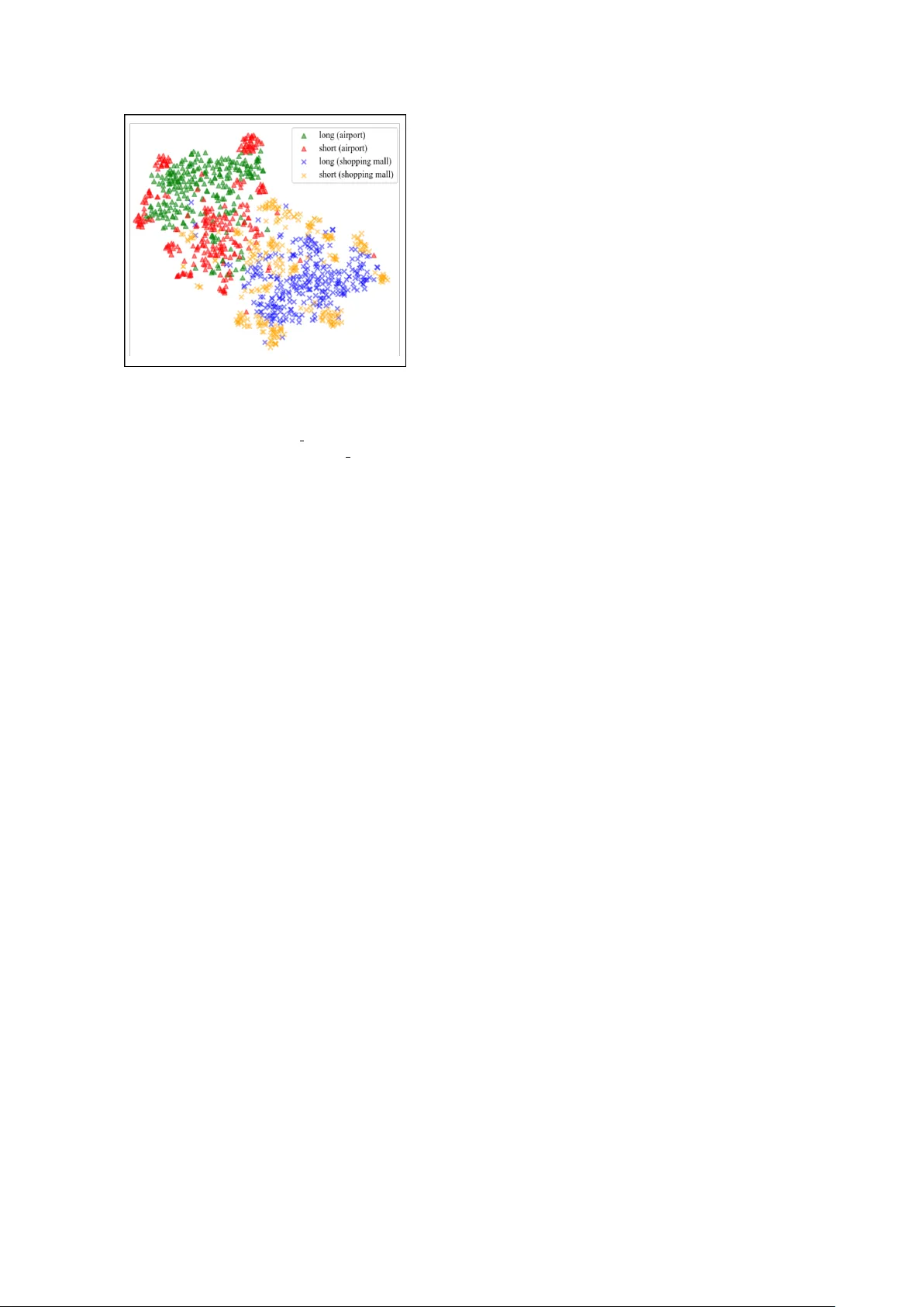
Acoustic scene classification using teacher -student learning with soft-labels Hee-Soo Heo ∗ , J ee-weon Jung ∗ , Hye-jin Shim, and Ha-Jin Y u † School of Computer Science, Uni versity of Seoul, South K orea zhasgone@naver.com, jeewon.leo.jung@gmail.com, shimhz6.6@gmail.com, hjyu@uos.ac.kr Abstract Acoustic scene classification identifies an input segment into one of the pre-defined classes using spectral information. The spectral information of acoustic scenes may not be mutually exclusi ve due to common acoustic properties across different classes, such as babble noises included in both airports and shopping malls. Howe ver , con ventional training procedure based on one-hot labels does not consider the similarities be- tween different acoustic scenes. W e exploit teacher-student learning with the purpose to deriv e soft-labels that consider common acoustic properties among dif ferent acoustic scenes. In teacher -student learning, the teacher network produces soft- labels, based on which the student network is trained. W e in- vestigate various methods to extract soft-labels that better rep- resent similarities across dif ferent scenes. Such attempts in- clude extracting soft-labels from multiple audio segments that are defined as an identical acoustic scene. Experimental results demonstrate the potential of our approach, showing a classifica- tion accuracy of 77.36 % on the DCASE 2018 task 1 v alidation set. Index T erms : teacher-student learning, knowledge distillation, acoustic scene classification, deep neural networks 1. Introduction Acoustic scene classification (ASC) refers to a task that catego- rizes an input audio segment into one of the pre-defined acous- tic scenes (classes). The detection and classification of acoustic scenes and events (DCASE) community , the leading platform for ASC and several related tasks, defines 10 acoustic scenes : airport, park, metro station, etc [1]. Such classes possess com- mon acoustic properties, such as babble noises included in both airports and shopping malls. W ith adv ances in deep learning, various deep neural net- works (DNNs) are primarily exploited for the ASC task, which are executed in a supervised manner using one-hot labels. How- ev er, in the con ventional training scheme which use one-hot labels with an softmax output layer , the common properties among different classes cannot be considered. This is because each acoustic scene is trained to be orthogonal in the label space. Here, the term ‘orthogonal’ refers to having no corre- lation between any other labels. W e hypothesize that this strict training process is not ef ficient because it is opposite to the pro- cess of human perception. Humans can recognize that there is a similarity between dif ferent acoustic scenes. This inefficienc y of the one-hot label technique can give rise to issues in most identification tasks, which would be further intensified in tasks, such as ASC, where the boundaries or definitions of the scenes ∗ These authors contributed equally † Corresponding author This research was supported by Basic Science Research Program through the National Research Foundation of Korea(NRF) funded by the Ministry of Science, ICT & Future Planning(2017R1A2B4011609) are ambiguous. W e expected that the similarity of each scene would be reflected in the soft-label. One of the well-kno wn techniques that extract soft-labels is teacher-student (TS) learning. In the TS learning, the student network is trained using a soft-label from the teacher network rather than con ventional one-hot label. The TS framework was first proposed for model compression, but was found to be an ef- fectiv e scheme to deal with various issues in related tasks, such as compensating far-field utterances in speech recognition [2]. The key factor that leads the various applications of TS learn- ing was an appropriate modification of the framework to suit the purpose. Therefore, we exploited various modifications of TS learning and e valuated them to consider common properties among different classes in the ASC task. W ith the inspiration from the pre vious researches [2, 3], we explored two techniques to modify the TS learning to better conduct the ASC task. The first is extraction of soft-labels from multiple input segments. This method enables extracting more general soft-labels and also includes the effect of data augmen- tation. The second is direct comparison of embeddings rather than the output layer , proposed in [3], was applied for the ASC task. W e verified that the combination of the two techniques can further improv e the performance of the ASC system. The rest of the paper is organized as follows. Section 2 describes the ov erall system, mainly front-end DNN and back- end support vector machine (SVM), used in this study . The TS learning scheme and the proposed techniques are discussed in Section 3. Section 4 presents the experiment and analysis results, and the paper is concluded in Section 5. 2. System description This section describes the system used for the ASC task. W e use a con volutional neural network (CNN) to process the raw wa veform, and a CNN with a layer of gated units (CNN-GRU) to process spectrograms. These two front-end models extract a fixed-dimensional embedding from an input segment. W e used SVM as the back-end for the ensemble of the two models. The scheme for combining the two models using spectrograms and raw wa veforms follows that of the authors’ previous research in [4]. In addition, we ha ve impro ved the performance of the system through few modifications, such as the DNN architec- ture. T able 1 shows that the baseline systems used in this study outperform the previously reported baselines without the ap- plication of TS learning . 2.1. Extraction of CNN-GR U embedding State-of-the-art systems in the ASC task comprise deep archi- tectures, using CNNs and recurrent architectures [4–7]. The CNN model for raw waveforms adopts 1D conv olutional layers for direct processing of raw wav eforms. Utilizing vast audio segments with a high sampling rate, these systems are capable of extracting an embedding that is highly representati ve. T able 1: Classification accuracy (%) of individual systems and their score-sum ensemble in terms of fold 1 configuration on the validation set. System Jung et al. [1, 4] Impro ved baseline Raw wa veform 67.15 69.38 Spectrogram 66.24 72.73 i-vector 63.74 - Ensemble 73.82 74.42 T able 2: DNN ar chitectur e of raw waveform model with input sequence shape: ( 479999 × 2 ). Layer Output shape Kernel size Stride Con v1 39999 × 64 12 12 Res1 13333 × 64 3 1 Res2 4444 × 128 3 1 Res3 1481 × 128 3 1 Res4 493 × 128 3 1 Res5 164 × 128 3 1 Res6 54 × 128 3 1 Res7 18 × 128 3 1 GlobalPool 128 - - Dense1 64 128 × 64 - Output 10 64 × 10 - The DNN used in this study comprises residual con volu- tional blocks and a fully-connected layer similar to that of [8, 9]. In this architecture, the input segments are processed using con- volutional layers to extract the frame-level features. These em- beddings are then aggregated into an utterance-lev el feature by using a global max pooling layer . One fully-connected layer is then used to extract the embedding, followed by the out- put layer . After the training, the output layer is removed, and embeddings are extracted from the last fully-connected layer . T able 2 depicts the overall DNN architecture using ra w wav e- forms. W e used a CNN-GRU model with 2D conv olutional layers for processing spectrograms. In this model, a two-channel spec- trogram extracted from stereo audio is input to the CNN, and a fixed dimensional embedding is output via the GR U layer . The ov erall DNN architecture using spectrograms is depicted in T a- ble 3. T able 3: DNN ar chitectur e of spectr ogram model with input se- quence shape: ( 249 × 256 × 2 ). Layer Output shape Kernel size Stride Con v1 249 × 256 × 30 7 × 7 1 × 1 Res1 249 × 256 × 30 3 × 3 1 × 1 Res2 125 × 128 × 60 3 × 3 2 × 2 Res3 63 × 64 × 120 3 × 3 2 × 2 Res4 21 × 22 × 120 3 × 3 3 × 3 A vgPool 21 × 1 × 240 1 × 22 1 × 22 MaxPool 21 × 1 × 240 1 × 22 1 × 22 Concan 21 × 480 - - GR U 480 - - Dense1 64 480 × 64 - Output 10 64 × 10 - 2.2. SVM classification The DNNs with the output layer activ ated by the softmax func- tion are well-known as a high-performance classifier . How- ev er, the softmax values in the output layer do not represent the concept of confidence. In other words, the softmax values are “poorly calibrated” [10]. In case of a single DNN, this issue does not cause an y problems. Howe ver , when combining output results from multiple DNNs, this can cause problems because the outputs are not confidence scores. T o av oid this problem, we implemented a separate scoring phase using the SVM clas- sifier . In the scoring phase, the output layers of two models are remov ed and the outputs of the last hidden layer of each model are trained using one SVM for each model. Finally , the scores calculated from the tw o SVMs are av eraged for the ensemble of the raw wa veform and spectrogram-based models. 3. T eacher -student learning in ASC T eacher -student (TS) learning is a frame work that adopts two DNNs. In this scheme, a superior system (teacher DNN) is first trained using con ventional training scheme with one-hot la- bels. Superiority of the teacher DNN is determined depending on the target task, i.e., larger capacity for model compression. Then the output of the teacher DNN (referred to as soft-label) is used to train a student DNN [11]. Specifically , the output dis- tributions of the teacher and student DNNs are compared using Kullback-Leibler di vergence with the follo wing equation: T S org = − I X i J X j p T ( o j | x i ) log ( p S ( o j | x i )) , (1) where p T ( · ) and p S ( · ) are the output distrib utions of the teacher and student network, respectively , and x i refers to the i 0 th in- put. Eq. (1) refers to cross-entropy rather than KL-div ergence, but the same effect can be achie ved when training the student network (look [11], Section 3.1. for further details). The TS framework has been expanded to kno wledge distil- lation with the concept of temperature in [12]. In knowledge distillation, the temperature T adjusts the extent of soft-label utilization where a higher T softens the probability distribution. Hence, the original equation of TS learning is expanded by in- cluding temperature variable T as: T S T = − I X i J X j p T ( o j | x i ; T ) log( p S ( o j | x i )) , (2) p T ( o j | x i ; T ) = exp ( p T ( o j | x i ) /T ) Σ K k exp ( p T ( o k | x i ) /T ) , (3) 3.1. Concatenating multiple inputs One of the important issues in the TS learning scheme is to de- sign the superiority of the teacher network. In the study that pro- posed the TS scheme, large capacity of the teacher netw ork was the superiority for a model compression task [11]. For far-field compensation study , less noise and re verberation comprised the superiority where the utterances recorded from close talk and the utterances recorded from far-field are input to the teacher and the student respectiv ely [2, 14]. In our study , possession of additional recording from identical acoustic scenes is set as the superiority . For this superiority , additional recording from the same class is concatenated to e very utterance, and then used for extracting the soft-label. For instance, the soft-label of a Figure 1: Illustration of the superiority using multiple segments for longer duration for the teacher network. t-SNE [13] plot of embeddings extracted fr om test set se gments on the most con- fusing acoustic scene pair , ‘shopping mall-airport’. 4 and × symbols repr esent the embeddings of shopping mall and airport scene, respectively . Cohesion of long duration embeddings are str onger , demonstrating the superiority of teacher network’s in- put. student DNN with input utterance ‘ A ’ will be derived by con- catenating another utterance ‘B’ from the same class and then inputting to the teacher DNN. Here, utterance ‘ A ’ is input to the student DNN and concatenation of utterance ‘ A ’, ‘B’ is input to the teacher DNN to extract a soft-label. This scheme is repre- sented using the following equation: K L loss = − I X i J X j p T ( o j | x i,con ) log ( p S ( o j | x i,base )) , (4) where x i,base is the base segment and the input segment of the student network, and x i,con is the input segment of the teacher network constructed by concatenating the input segment of the student DNN with another segment from an identical class. In particular , the length of x i,base is fix ed to 10 s, and the duration of x i,con can be 20, 30 s, or longer . The superiority caused by concatenating multiple inputs is sho wn in detail in figure 1. The figure shows that the embeddings extracted from long segments have higher discriminativ e power . This superiority is also interpreted as that of short utterance compensation in the field of speaker verification [3, 15]. Deriving soft-labels using multiple audio recordings is also expected to include the effect of data augmentation. T rain- ing data augmentation, conducted by adding noises or shifting pitch, is a well-known technique for performance improvements in the audio processing tasks using DNNs. In the ASC task, howe ver , it is difficult to apply the conv entional data augmen- tation scheme because the definition of acoustic scene is am- biguous, and there is no clear approach to define which noise belongs to which class. In particular , adding babble noise to the training data can give rise to a critical issue that changes the class label of the training data. In the proposed approach, the input data of the teacher network is changed depending on the selection of inputs for concatenation where the input audio recording of the student network is fixed. Therefore, we ex- pected that there would be a similar ef fect of data augmentation through these combinations of multiple inputs. 3.2. Learning based on embeddings distance In the proposed ASC system introduced in Section 2, the soft- max output layer is removed after the training phase and the embeddings extracted from the last hidden layer are used for the scoring phase. Therefore, the last hidden layer, and not the output layer, is a more dominant factor in the performance of the ASC system. Based on this property , we modified the TS learning to take into account the output of the last hidden layer as follows: T S emb = J X j D ist ( E T ( x j ) , E S ( x j )) , (5) where D ist ( · ) is the distance measure between two vectors, and E T ( · ) and E S ( · ) are the output of the last hidden layer from the teacher and the student network, respectiv ely . In this study , we used mean squared error as the distance measure. W e inter- preted this approach as the distilling the knowledge at the last hidden layer , and not at the output layer . This approach was inspired by [3] and [2]. 4. Experiments and results In this section, we show the results of experiments to ev alu- ate the various TS learning techniques. The baseline system used for the performance comparison is an improv ed version of the authors’ system that was presented at the last DCASE 2018 competition (see T able 1). Therefore, we focused on e valuat- ing the effecti veness of the TS learning rather than comparing it with other systems. 4.1. Dataset DCASE 2018 task 1-a dataset [1] was used for all experiments in this study . This dataset comprises 864 audio segments that has 10 s duration for each of 10 pre-defined classes, resulting in a total of 8640 segments. The audio segments were recorded in stereo at a sampling rate of 48 kHz. Cross-validation was conducted using the four fold configuration provided within the DCASE dataset, where the validation sets are recorded from different locations. 4.2. Experimental settings All experiments in this study were conducted using Keras, a deep learning library for python, with T ensorflow back-end [16– 18]. For the raw wav eform model, pre-emphasis is applied [19] without any other pre-processing. The whole segment is input, which makes the shape of input segment as (479999 , 2) . The DNN architecture configuration is depicted in T able 2. W e e xtracted the spectrograms of 256 coef ficients from 100 ms windo ws for every 40 ms. The spectrogram of (249 , 256 , 2) shape w as e xtracted for each segment that contains stereo audio of 10 s. Adam optimizer [20] with 0.001 learning rate was used for training both CNN using raw waveforms and CNN-GR U using spectrograms. The batch size for training the two models was 40. For efficient training of the spectrogram-based CNN-GR U model, we trained the CNN part except the GRU layer in the whole model and then re-trained after attaching the GR U layer on the CNN, following the multi-step training scheme reported in [9, 21]. Figure 2: Confusion matrices before (left) and after (right) ap- plying the proposed TS learning scheme. Both of the two most confusing acoustic scene pairs, ‘shopping mall-airport’ (red box) and ‘metr o-tram’ (gr een box) show impro vement. 4.3. Analysis of results T able 1 demonstrates the baseline of this study , which is an improv ed version of the authors’ submission to DCASE 2018 competition. The individual systems show improv ed perfor- mance. For the ensemble, “Improv ed baseline” outperforms the previous baseline despite the i-v ector [22] system is excluded. T able 4 sho ws the performances of spectrogram-based models using TS learning with various temperature T and input durations. The temperature coefficient T , described in equation (2), is an important factor that determines the extent of soft- label utilization. As the value of T increases, the output dis- tribution of the teacher network becomes more noisy . On the contrary , decrease in the value of T refers to imposing more weight to the one-hot (hard) label. Comparing the results when T v alues is one and five, we interpret that to some extent, con- sidering common properties is important. It is also important to design the superiority of the teacher network in the TS learning scheme. This is because the train- ing process of the student network is totally dependent on the teacher network. Howe ver , the teacher network, trained using one-hot labels, may hav e poor performance. Even the teacher network may distill wrong knowledge to the student network. Experimental results showed that adjusting the input length of the teacher network to gain superiority could lead to perfor- mance improv ements as intended. T able 4: P erformance in terms of accuracy (%) depending on temperatur e T and superiority of the teacher network. Duration of teacher input 10 seconds 20 seconds T 1 70.96 71.43 5 72.63 73.23 10 72.51 72.79 T able 5 demonstrates the ef fectiv eness of direct comparison of the embeddings between the teacher and student networks. The results show that use of the embedding of teacher DNN outperforms the soft-label of the output layer . Use of both soft- label and embedding layer , ho wev er, shows decreased accuracy . W e interpret that this phenomenon occurred because the com- mon properties across dif ferent classes are better represented in the embedding space rather than using human defined one-hot labels. For example, the soft-label generated at the output layer represents the common properties, such as babble noise depend- ing on the corresponding classes (airport or shopping mall), b ut the soft-label at the last hidden layer can represent the common property by manifold in a high dimensional embedding space. T able 5: P erformance depending on points of knowledge distil- lation. Point accuracy (%) output layer 73.23 output & last hidden layer 73.19 last hidden layer 74.26 T able 6 shows the comparison of the approaches used in this study to the baseline. The proposed approach with TS learning demonstrates classification accuracy of 77.36 % compared to 74.42 % for the scheme without TS learning. From these re- sults, we conclude that the TS learning scheme is effecti ve for the ASC task, and the approaches developed in this study are also valid. T able 6: Classification accur acy of individual systems and their scor e-sum ensemble in terms of fold 1 configuration on the val- idation set (W/O TS: systems trained without TS learning, W/ TS: systems trained with TS learning). System W/O TS W/ TS Raw wa veform 69.38 72.99 Spectrogram 72.59 74.26 Ensemble 74.42 77.36 W e analyzed the detailed contribution of performance en- hancement by TS learning. Figure 2 illustrates two confusion matrices, with and without applying the proposed TS learning scheme, which shows that TS learning significantly reduced the errors between the two most confusing acoustic scene pairs. 5. Conclusions and discussion The con ventional training procedures using one-hot label can- not represent common properties among different classes. W e assume that this scheme is not appropriate for tasks such as the ASC where the decision boundary of each class is ambiguous. Therefore, we explored various applications of TS learning to use the soft-label instead of the one-hot label. W e applied TS learning to the ASC task for the first time based on two tech- niques: using multiple segments for the teacher network and distilling the knowledge at the last hidden layer . In TS learning, the student network is trained using soft-labels extracted from the teacher network. Soft-label in TS learning was interpreted to incorporate the correlation of different acoustic scenes with common acoustic properties. W e ev aluated various approaches of TS learning using the DCASE 2018 task 1 dataset. Experi- mental results demonstrate that designing the superiority of the teacher network and adjusting the point of knowledge distilla- tion could improv e the performance. In particular , TS learn- ing significantly reduced the errors between the most confusing scenes. 6. References [1] A. Mesaros, T . Heittola, and T . V irtanen, “ A multi-device dataset for urban acoustic scene classification, ” 2018, submitted to DCASE2018 W orkshop. [Online]. A vailable: https://arxi v .org/ abs/1807.09840 [2] J. Kim, M. El-Khamy , and J. Lee, “Bridgenets: Student-teacher transfer learning based on recursive neural networks and its ap- plication to distant speech recognition, ” in 2018 IEEE Interna- tional Conference on Acoustics, Speech and Signal Pr ocessing (ICASSP) . IEEE, 2018, pp. 5719–5723. [3] J.-w . Jung, H.-s. Heo, H.-j. Shim, and H.-j. Y u, “Short ut- terance compensation in speaker verification via cosine-based teacher-student learning of speaker embeddings, ” arXiv pr eprint arXiv:1810.10884 , 2018. [4] ——, “DNN based multi-lev el feature ensemble for acous- tic scene classification, ” in Proceedings of the Detection and Classification of Acoustic Scenes and Events 2018 W orkshop (DCASE2018) , November 2018, pp. 113–117. [5] Y . Sakashita and M. Aono, “ Acoustic scene classification by en- semble of spectrograms based on adaptive temporal di visions, ” DCASE2018 Challenge, T ech. Rep., September 2018. [6] M. Dorfer, B. Lehner, H. Eghbal-zadeh, H. Christop, P . Fabian, and W . Gerhard, “ Acoustic scene classification with fully con vo- lutional neural networks and I-vectors, ” DCASE2018 Challenge, T ech. Rep., September 2018. [7] H. Zeinali, L. Burget, and H. Cernock y , “Conv olutional neural networks and x-vector embedding for dcase2018 acoustic scene classification challenge, ” DCASE2018 Challenge, T ech. Rep., September 2018. [8] J. Jung, H. Heo, I. Y ang, H. Shim, and H. Y u, “ A complete end- to-end speaker verification system using deep neural networks: From raw signals to verification result, ” in 2018 IEEE Interna- tional Conference on Acoustics, Speech and Signal Pr ocessing (ICASSP) . IEEE, 2018, pp. 5349–5353. [9] ——, “ A voiding speaker overfitting in end-to-end dnns using raw wav eform for text-independent speaker verification, ” in Proc. In- terspeech 2018 , 2018, pp. 3583–3587. [10] C. Guo, G. Pleiss, Y . Sun, and K. Q. W einberger , “On calibration of modern neural networks, ” arXiv preprint , 2017. [11] J. Li, R. Zhao, J. Huang, and Y . Gong, “Learning small-size dnn with output-distribution-based criteria, ” in Fifteenth annual con- fer ence of the international speech communication association , 2014. [12] G. Hinton, O. V inyals, and J. Dean, “Distilling the knowledge in a neural network, ” arXiv preprint , 2015. [13] L. Maaten and G. Hinton, “Visualizing data using t-sne, ” Journal of machine learning r esearc h , vol. 9, no. Nov , 2008. [14] J. Li, R. Zhao, Z. Chen, C. Liu, X. Xiao, G. Y e, and Y . Gong, “De- veloping f ar-field speaker system via teacher -student learning, ” in 2018 IEEE International Conference on Acoustics, Speech and Signal Pr ocessing (ICASSP) . IEEE, 2018, pp. 5699–5703. [15] H. Y amamoto and T . Koshinaka, “Denoising autoencoder-based speaker feature restoration for utterances of short duration, ” in Sixteenth Annual Conference of the International Speech Com- munication Association , 2015. [16] F . Chollet et al. , “Keras, ” https://github.com/keras- team/k eras, 2015. [17] A. Mart ´ ın, A. Ashish, B. Paul, B. Eugene et al. , “T ensorflow: Large-scale machine learning on heterogeneous distrib uted systems, ” 2015. [Online]. A vailable: http://download.tensorflo w . org/paper/whitepaper2015.pdf [18] A. Martin, B. Paul, C. Jianmin, C. Zhifeng, D. Andy , D. Jeffrey , D. Matthieu, G. Sanjay , I. Geoffrey , I. Michael, K. Manjunath, L. Josh, M. Rajat, M. Sherry , M. G. Derek, S. Benoit, T . Paul, V . V ijay , W . Pete, W . Martin, Y . Y uan, and Z. Xiaoqiang, “T ensorflow: A system for large-scale machine learning, ” in 12th USENIX Symposium on Operating Systems Design and Implementation (OSDI 16) , 2016, pp. 265–283. [Online]. A vailable: https://www .usenix.org/system/ files/conference/osdi16/osdi16- abadi.pdf [19] R. V ergin and D. O’Shaughnessy , “Pre-emphasis and speech recognition, ” in Electrical and Computer Engineering, 1995. Canadian Confer ence on , vol. 2. IEEE, 1995, pp. 1062–1065. [20] D. P . Kingma and J. Ba, “ Adam: A method for stochastic opti- mization, ” arXiv pr eprint arXiv:1412.6980 , 2014. [21] H. S. Heo, J. W . Jung, I. H. Y ang, S. H. Y oon, and H. J. Y u, “Joint training of expanded end-to-end DNN for text-dependent speaker verification, ” Proc. Inter speech 2017 , pp. 1532–1536, 2017. [22] N. Dehak, P . Kenny , R. Dehak, P . Dumouchel, and P . Ouellet, “Front-end factor analysis for speaker verification, ” IEEE T rans- actions on Audio, Speech, and Language Processing , vol. 19, no. 4, pp. 788–798, 2011.