Model-Free Active Input-Output Feedback Linearization of a Single-Link Flexible Joint Manipulator: An Improved ADRC Approach

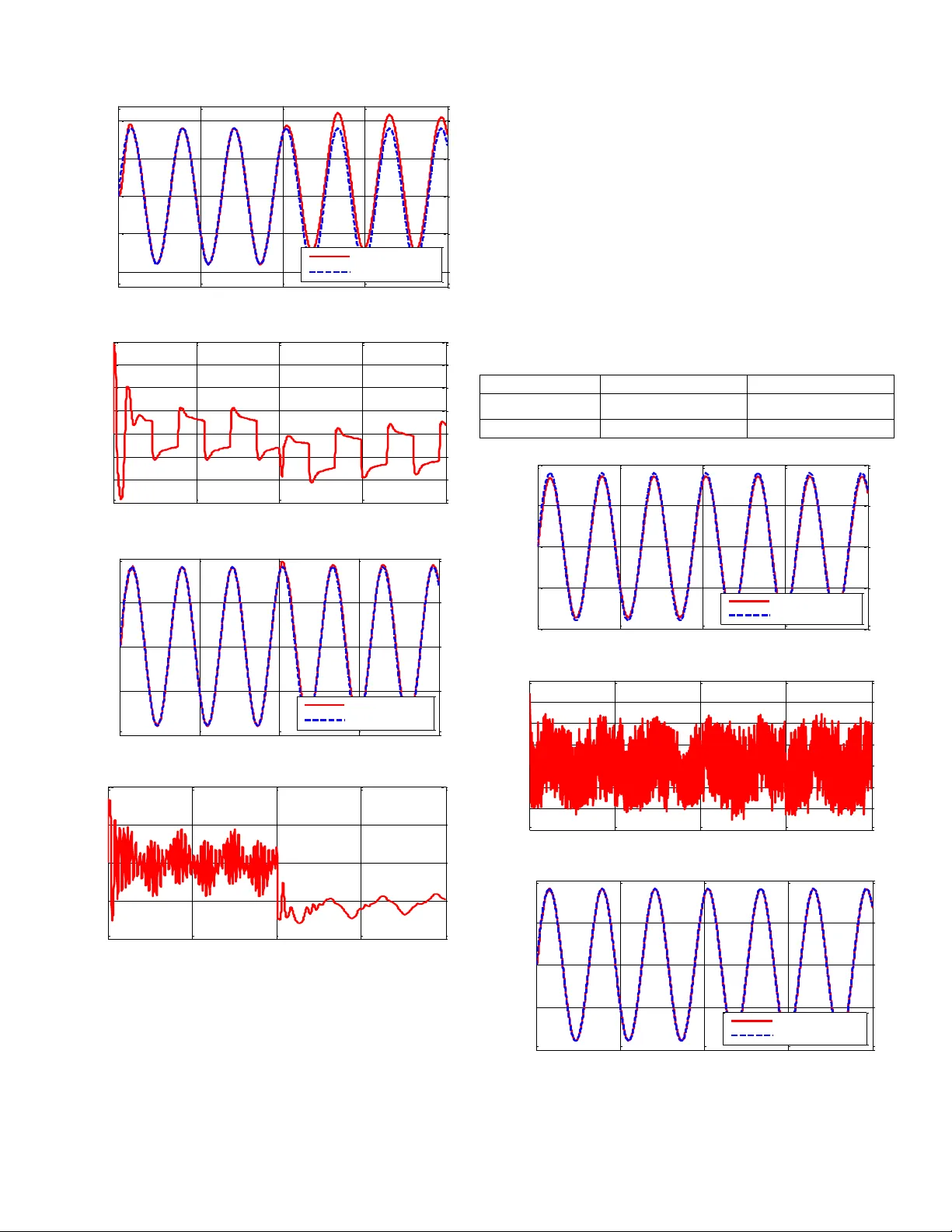
1 On The Active Input-Output Feedback Linearization of Single-Link Flexible Joint Manipulator : An Extended State Observer Approach Wameedh Riyadh Abdul-A dheem Ibraheem Kasim Ibraheem Electrical Engineering De partment Electrical Enginee ring Department College of Engineeri ng, Baghdad University College of Engineering, Bagh dad University Baghdad, Iraq Baghdad, Iraq Wameedh.r@coeng.uobag hdad.edu.iq ibraheem ki@coeng.uobaghdad.edu.iq Abstract — Traditional input-output feedback linearization (IOFL) is an essential part of nonlinear control theory and a valuable tool in solving class of problems possessing certain constraints. It requires full knowledge of system dynamics and assumes no disturbance at the input channel and no system's uncertainties. In this paper, an Active Input-Output Feedback Linearization (AI OFL) technique based on extended state observer which is the core part of the Active Disturbance Rejection Control (ADRC) paradigm is proposed to design a feedback linearization control law. This control law transforms the system into a chain of integrators up to the relative degree of the system. The proposed AIOFL simultaneously cancels the generalized disturbances (exogenous disturbance and internal uncertainties) and delivers the estimated system ’s states to the nonlinear state error feedback of the ADRC. Verification of the outcomes has been achieved by applying the proposed technique on the ADRC of Flexible Joint Single Link Manipulator(SLFJM). The results show ed the effectiveness of the proposed tool. Keywords — Active input-Output feedback lineariz ation, Extended state observer, flexible joint, generalized disturbance, tracking differentiator. I. I NTRODUCTION There are numerous classe s of nonlinear models. Given the following one,   󰇗   󰇛  󰇜   󰇛  󰇜     󰇛  󰇜   (1 ) Where   󰇛        󰇜     is the state vector,    is the control input an d    , is the system output. The functions      are sufficiently smooth in a domain     . The mappings        and       are called vector fields on  . C onsider the Jacobian linearization of the system (1) about the equilibrium point 󰇛        󰇜 ,   󰇗    󰇛  󰇜    󰇛  󰇜     󰇛     󰇜   󰇛   󰇜󰇛     󰇜       󰇛   󰇜  󰇛     󰇜   It is worthy to observe that the nonlinear system is accurately represented by the Jacobian model only at the equilibrium point 󰇛        󰇜 . Consequently, a ny control po licy built on the linearized model may produce inacceptable performance at other operating points. Fee dback lineariz ation (FL) is another class of nonlinear control m ethods that can yields linear models that is a pr ecise depiction of the fundamental nonlinear model among a wide set of the equilibrium points [1] . Simply, FL is a technique, which elim inates all the nonlinearit ies with the result that the nonlinear dynamical system is represented by a chain of integrators. FL can be ap plied in three steps, the first step is transforming the nonli near system into a linea rized m odel , this is achieved through appropriate nonlinear change of variables. After this stage, the equations of the system are linear but with the cost of a nonlinear control law( u ) w hich converts the system into a chain of integrators up to the relative degree of the system with linear control law( v ). The second step is applying one o f traditional linear control methods such as state-feedback, PID control, etc ., to control the linearized model. The third step is the stability investigation of the internal dynamics [2]. FL has been applied in recent years in various research and industrial fields , for exam ple, in t he control of induction motors [3], spacecraft models that includes reaction wheel configuration [4], surface permanent-magnet-synchro nous generator (SPMSG) [5]. Further applications include, m aximum po wer point tracking (MPPT) technique to achieve the desired performance under sudden irradiation drops, set-point changes, and load disturbances [6], Adapti ve Input-Output Feedback Linearization (AIOFL) to damp the low -frequency oscillations in power systems [7] and for the reduction of torque ripple of a brushless DC motors [8]. Finally , in robust nonlinear controller design for the voltage-source converters of high-voltage, direct current transmission link using IOFL an d sliding-mode control approach [9] . This paper proposes a method for Input-Output Feedback Linearization (IOFL) in an active manner, namely, the AIOFL , in which the nonlinearities, model uncertainties, and external disturbance are excellently estimated and canceled, resulting the nonlinear system is reduced into a chain of integrators up to the relative degree of the syst em. The key points of the propose d method are, AIOFL requires only the relative degree of the nonlinear system in contrast to conventional feedback linearization, which requires complete knowledge of the 2 nonlinear syst em to design the linearizing control law. The second key point is that ther e is no need to do any diffeomorphism transformation. Finally, on contrast to conventional IOFL, the proposed AIOFL is hi ghly imm une against uncertainties an d external disturbances. This paper is organized as follows. In section II a brief introduction to ADRC is presented. Background and problem statement are introduced in section III. In section IV Active Input- Output Feedback Linearization is discussed with detailed proofs. In section V, the single link flexible joint manipulator is presented as a guideway example for the proposed method. Finally, the conclusions are drawn i n section VI. II. E XTENDED S TATE O BSERVER Extended State Observer (ESO) is the central part of a recent robust control paradigm, the so-called ADRC . It is an advanced robust control strategy, which works by augmenting the mathematical model of the nonlinear dynamical system with an additional virtual state. This virtual state describes all the unwanted dynam ics, uncertainties, and exogenous dist urbances and named the “ generalized disturbance ” or “ total disturbance ” . This virtu al state together with the states of the dynamic system are observed in real-time fashion using the ESO . It performs direct and active prediction and cancelation to the total disturbance by feeding back the estimated generalized disturbance into the input channel after simple m anipulation. With ADRC , controlling a complex time-varying nonlinear system is transformed into a simple and linearized process. The superiority that makes it such a successful robust control tool is that it is an error-driven technique, rather t han model-based control law. Mainly, ADRC co nsists of an ESO, a tracking differentiator (TD), and a nonlinear state error combination (NLSE F) as illustrated in Fig. 1 [10] – [12 ]. Where    is the reference input, 󰇛       󰇜     is the transient profile ,    is the control input for the linearized model, 󰇛           󰇜     is the augmented estimated vector which comprises the plant’s states           and the estimated generalized disturbance    , which are produced by the extended state observer and   is the input gain. Fig. 1 Structure of ADRC. Statement of contribution . The contribution of this paper is developing the AIOFL technique based on the ESO. We use the ESO not just as an estimator for the total disturba nce (    ) which later on will be rejected as shown in Fig. 1, but, also as a linearization tool. The nonlinear sliding mode ESO developed in our previous work [12] will be used in this work in addition to the linear ESO (LESO). T he advantage of this tech nique is that it transforms any nonlinear uncertain system with exogenous disturbance into a chain of integrators up to the relative de gree of the system. The proposed AIOFL method is effective due its simplicity. For linearization, the only required information is the relative order of the system . III. BAC KGROUND AND PROBLEM STAT EMENT To perform IOFL , conditions have to be derived and stated which allow us to do the transformation to the nonlinear system such that the input-output m ap is linear. Given  󰇗 as,  󰇗  󰇛 󰇜   󰇗    󰇟  󰇛  󰇜   󰇛  󰇜  󰇠     󰇛  󰇜     󰇛  󰇜  Where    󰇛  󰇜     󰇛  󰇜  is called the Lie De rivative of  󰇛  󰇜 with respect to f . If    󰇛  󰇜   , then  󰇗     󰇛  󰇜 is independent of u . The second derivative of y , den oted by  󰇘 is given by  󰇘       󰇗      󰇟  󰇛  󰇜   󰇛  󰇜  󰇠      󰇛  󰇜       󰇛  󰇜  Once again, if      󰇛  󰇜   , then  󰇘      󰇛  󰇜 , is also independent of u . Repeating t his process with  󰇛  󰇜 , one gets, 󰇫       󰇛  󰇜                 󰇛  󰇜   (2) It can be seen that u is not included in    󰇗     󰇛󰇜 but  󰇛󰇜  with a nonzero coefficient,  󰇛󰇜      󰇛  󰇜        󰇛  󰇜  . The control signal          󰇛  󰇜     󰇛  󰇜    reduces the input-output map to  󰇛󰇜   . The system is obviously input- output feedback linearizable, i.e. the nonlinear system (1) is represented by a chain of integrators, wh ere  is denoted as the relative degree of the nonline ar system. Now let    󰇛  󰇜         󰇛󰇜    󰇛 󰇜    󰇛 󰇜     󰇛 󰇜        󰇛 󰇜    󰇛 󰇜          (3 ) Where   󰇛 󰇜 to   󰇛 󰇜 are chosen such that   󰇛󰇜   󰇛  󰇜      󰇝       󰇞    This condition ensures that when the followi ng equatio n is cal culated  󰇗   󰇛 󰇜  󰇟  󰇛  󰇜   󰇛  󰇜  󰇠    󰇛    󰇜    󰇛    󰇜  , the term u cancels out. It is now easy to verify that    󰇛  󰇜  transforms the system into normal form denoted as       󰇗    󰇛   󰇜   󰇗       󰇝       󰇞   󰇗    󰇛  󰇜   󰇛  󰇜        Where  󰇛  󰇜      󰇛  󰇜  󰇛  󰇜        󰇛  󰇜  The internal dynamics are described by  󰇗    󰇛   󰇜 . The ze ro-dynamics of the system is sta ted as  󰇗    󰇛    󰇜 with ξ = 0 ( i.e .,  󰇗    󰇛    󰇜 ). 3 The system is called minimum phase if the zero-dynamics of the system are (globally) asy mptotically stable. IV. A CTIVE INPUT - OUTPUT FEEDBACK LINE ARIZATION Consider the nonlinear SISO syst em given as  󰇛󰇜 󰇛  󰇜    󰇛  󰇜  󰇛  󰇜     󰇛  󰇜 󰇛  󰇜   󰇛  󰇜      󰇛 󰇜 󰇛 󰇜 where  󰇛 󰇜 󰇛  󰇜 indicates i th derivative of y (the output), and d and u represent the disturbance and the input, respectively. Many classes of nonlinear systems can be represented in this no tation, e.g., time-varying or time-invariant systems, nonlinear or linear systems. For simpler repres entation and without causin g any ambiguity, the time var iable will be omitted from the equations. Assuming          󰇗        󰇛󰇜 , one gets         󰇝       󰇞   󰇗    󰇡              󰇢  󰇛  󰇛  󰇜    󰇜       (4) Augmenting the system with additional state,      󰇛  󰇛  󰇜    󰇜        󰇗   󰇛 󰇜   󰇗  . The coefficient   is a rough approximation of  󰇛 󰇜 in the plant within a ±50% range [10] and      󰇛  󰇛  󰇜    󰇜  is the generalized disturbance, which consists all of the unknown external disturbances , uncertainties and internal dynamics. The parameter   usually chosen explicitly by the user as a design parameter. The states of the system in (4) together with the generaliz ed disturbance   will be estimated by the ES O, given by [13], [14],        󰇗                   󰇝       󰇞   󰇗                      󰇗             (5) The noteworthy feature of the ESO is t hat it needs minim um information about the dynamic al system, only  of the underlying system is needed to the design of the ESO. Severa3l modificat ions have been de veloped to e xpand the basic features of ESO to adapt to a broader class of dynamic al systems [13] . In this section, the convergence of the Linear ESO (LESO) is considered. Consider the system (4) with the augm ented state   is given as:         󰇝       󰇞   󰇗          󰇗   󰇛󰇜    󰇗   (6) Assumption (A1): T he funct ion   is continuously differentia ble Assumption (A2): T here exist a positive constant  suc h that   󰇛  󰇜   for    Assumption (A3) [14] : There exist constants      and positive definite, continuous ly differentiable functions          such that:         󰇛  󰇜          󰇛  󰇜      , (7)      󰇛        󰇜             󰇛 󰇜 . (8) Lemma 1. Consider the candidate Lyapunov functions          defined by  󰇛  󰇜      , where     and  is a symmetric posit ive definite m atrix. Suppose that (7) in Assumption (A3) with      󰇛󰇜 and      󰇛󰇜 , where   󰇛󰇜 and   󰇛󰇜 are the minimal and maximal eigenvalues of  , respectively . Then, (i).         󰇛󰇜    , (ii)  󰇛 󰇜   󰇛 󰇜   󰇛  󰇜 (iii)      󰇛 󰇜   󰇛󰇜 . Proof: (i) Since  󰇛  󰇜    󰇛󰇜     and 󰇻    󰇻  󰇼  󰇛 󰇜  󰇼 , then         󰇛󰇜    , (ii)Since  󰇛  󰇜    󰇛  󰇜       󰇛  󰇜  󰇛 󰇜 , then,  󰇛 󰇜   󰇛  󰇜   󰇛  󰇜 , and (iii) Since,   󰇛󰇜       󰇛 󰇜 , then,      󰇛 󰇜   󰇛󰇜 . 󰅾 Theorem 1. Given the chain of integrators system given in (6 ), and t he ESO in (5). Then, under Assumptions (A1)-(A3), for any initial values,        󰇛󰇜   󰆹  󰇛󰇜   ,   󰇝   󰇞    󰆹                    󰇛  󰇛  󰇜    󰇜     where   󰇛󰇜 , and  󰆹  󰇛󰇜 denote the solutions of ( 6) and (5) respectively,   󰇝     󰇞 . Proof: we make use of [14] to prove t he convergence for t he LESO. Set   󰇛  󰇜    󰇛  󰇜   󰆹  󰇛󰇜 , for   󰇝     󰇞 . T hen subtracting (5) from (6 ), one gets           󰇗  󰇛  󰇜   󰆹 󰇗  󰇛  󰇜    󰇛  󰇜   󰆹  󰇛  󰇜    󰇡 󰇛  󰇜   󰆹  󰇛  󰇜 󰇢                 󰇗  󰇛  󰇜   󰆹 󰇗  󰇛  󰇜    󰇛  󰇜   󰆹  󰇛  󰇜    󰇛 󰇛  󰇜   󰆹  󰇛  󰇜 󰇜                    󰇗  󰇛  󰇜   󰆹 󰇗  󰇛  󰇜    󰇛  󰇜     󰇛  󰇜           󰆹  󰇛  󰇜     󰇛  󰇜    󰇡 󰇛  󰇜   󰆹  󰇛  󰇜 󰇢             󰇗  󰇛  󰇜   󰆹 󰇗  󰇛  󰇜   󰇛  󰇜    󰇛 󰇛  󰇜   󰆹  󰇛  󰇜 󰇜              Direct computations show that the estimated error dynamics satisfy:       󰇗  󰇛  󰇜    󰇛  󰇜     󰇛  󰇜   󰇗  󰇛  󰇜    󰇛  󰇜     󰇛  󰇜    󰇗  󰇛  󰇜    󰇛  󰇜     󰇛  󰇜   󰇗  󰇛  󰇜   󰇛  󰇜     󰇛  󰇜  (9 ) Let         , where   ,   󰇝     󰇞 is the associated constant with e ach    , , and   is the bandwidth. The fi nal form with   substituted in (9) is given as:       󰇗  󰇛  󰇜    󰇛  󰇜        󰇛  󰇜   󰇗  󰇛  󰇜    󰇛  󰇜         󰇛  󰇜    󰇗  󰇛  󰇜    󰇛  󰇜         󰇛  󰇜   󰇗  󰇛  󰇜   󰇛  󰇜         󰇛  󰇜   ( 10 ) We ass ume   󰇛  󰇜       󰇛    󰇜 ,   󰇝     󰇞 [16 ].   󰇡    󰇢        󰇛  󰇜 (11) 4 Then time-scaled estimation error dynamic s are expressed as:          󰇛  󰇜     󰇛  󰇜      󰇛  󰇜    󰇛  󰇜     󰇛  󰇜      󰇛  󰇜      󰇛  󰇜     󰇛  󰇜      󰇛  󰇜     󰇛  󰇜           󰇛  󰇜  (1 2) Finding  󰇗 (the differentiation of  󰇛  󰇜 ) w.r.t t over  (over the solution ( 12 ) ) is accomplished in the following way  󰇗 󰇛  󰇜  󰇛  󰇜    󰇛  󰇜      󰇗  󰇛󰇜    󰇛  󰇜       󰇛  󰇜      󰇛  󰇜    󰇛  󰇜            󰇛  󰇜  Then,  󰇗 󰇛  󰇜  󰇛  󰇜    󰇛  󰇜       󰇛  󰇜      󰇛  󰇜    󰇛  󰇜        󰇛  󰇜       󰇛  󰇜 If the second inequality i n Assumption (A3) is satisfied, then  󰇗 󰇛  󰇜  󰇛  󰇜   󰇛 󰇜   󰇛  󰇜      Given that the rate of change of the generalized disturbance is bounded (Assumption (A2)) and the res ults of Lemma 1, we get:  󰇗 󰇛  󰇜   󰇛 󰇜   󰇛  󰇜       󰇛󰇜  󰇛 󰇜    󰇛  󰇜 ( 13 ) knowning that     󰇛 󰇜      󰇛 󰇜  󰇗 󰇛  󰇜 , then (13) is an ordinary 1 st order differential equation ( 13 ), its solution can be fo und as,   󰇛 󰇜     󰇛  󰇜      󰇛  󰇜        󰇛  󰇜     󰇛 󰇛󰇜󰇜     󰇛  󰇜   󰇛󰇜       󰇛  󰇜      󰇛  󰇜      󰇛  󰇜        󰇛  󰇜      󰇛 󰇛󰇜󰇜     󰇛  󰇜    󰇛󰇜       󰇛  󰇜     󰇛  󰇜        󰇛  󰇜    󰇛 󰇛󰇜󰇜   󰇛  󰇜      󰇛  󰇜 . It follows from ( 11 ) that   󰇛󰇜   󰆹  󰇛󰇜         󰇛    󰇜    󰇛󰇜   󰆹  󰇛󰇜        󰇛 󰇜  . Then, we get,   󰇛  󰇜   󰆹  󰇛  󰇜           󰇛  󰇜     󰇛  󰇜        󰇛  󰇜    󰇛 󰇛󰇜󰇜   󰇛  󰇜      󰇛  󰇜  . Finally,        󰇛󰇜   󰆹  󰇛󰇜 =0 a nd    󰆹                    󰇛  󰇛  󰇜    󰇜    󰅾 If the linearization control law (LCL)  is selected as          and as result of theorem 1, t hen, the nonlinear system in (4) is reduced to a chain of  integrators desc ribed as,        󰇝       󰇞  󰇗      (14) The main differences between IOFL and AIOFL are , for the AIOFL, there is no need to obtain the transformation of (3). The only requi red informat ion is t he relative degree of t he system 󰇛󰇜 for the nonlinear system to be linearized. While, for the IOFL , transformation (3) is the key step to linearize the system, it is based on exact mathematical cancelation of the nonlinear terms  󰇛 󰇜 and  󰇛 󰇜 , which requires knowledge of  ,  , and T . Furthermore, AIOFL in addition to linearizing the nonlinear system, it lumps the external disturbances, uncertai nties, and unmodeled dynamics , into a single term for online and active estimation and cancelation lat er on . V. G UIDE W AY E XAMPLE In this example, a SISO single-link flexible joint manipulator ( SLFJM) offered by [15] is studied and shown in Fig. 2 . The state- space representation of the SLFJM system in the form of the nonlinear system given in (1) is described as,   󰇗   󰇛  󰇜             Where   󰇛         󰇜   󰇛    󰇗  󰇗 󰇜     is the plant state,    the plant input,     the exogenous disturbance,     the plant output, and       . The components of       are denoted, respectively, by             󰇛  󰇜                                                              󰇛     󰇜        󰇡                    󰇢      󰇡          󰇢     󰇛     󰇜  (15) Where   is t he link stiffness,   is the inertia of hub,  is the li nk mass,  is the height of hub,   is the motor constant,   is the gear ratio,   is the load inertia, and    is the motor resistance. The values of the coefficients for SLFJM are [15]:    1.61 ,    0.0021 ,    0.403 , g  -9.81,   0.06 ,    0.00767,    70,    0.0059, and    2.6 . Apply ing the Lie derivative on equation (5 ), we get the following set of equations [16]:    󰇛  󰇜   ,       󰇛  󰇜         󰇛  󰇜   ,       󰇛  󰇜   It can be noticed that the SLFJM system in (15) satisfie s (2); consequently, the relative order of SLFJM is 4, i.e.,    [16]. Two types of ESOs are tested in this paper. The conventional ADRC is the com bination of th e Linear ESO(LESO) given by (16), NLSEF was given by (17), and TD given by (18). According to [13], [14] , a LESO observe r can be designed as:     󰆹 󰇗    󰆹        󰆹    󰆹 󰇗    󰆹        󰆹    󰆹 󰇗    󰆹        󰆹    󰆹 󰇗    󰆹        󰆹        󰆹 󰇗        󰆹   (16) 5 Fig. 2 Definition of generaliz ed coordinates for the SLFJM Where  󰆹    󰆹   󰆹   󰆹   󰆹   󰆹    is the observer ’s state vector, and   󰇛           󰇜   󰇛                        󰇜 T is the observer gain vector. The control law for the AIOFL is given as,              󰇛         󰇜   󰇛         󰇜 , with  󰇛      󰇜  󰇫               󰇛 󰇜      (17) where   󰇛     󰇜  is the tracking error vector which can be defined as        󰆹  with i = 1, 2 . The nonlinear second order differentiator is given as [ 11 ] : 󰇫  󰇗       󰇗    󰇛    󰇛  󰇜          󰇜 (18) Where r 1 is tracking signal of the input r , and r 2 tracking signal of the derivative of the input r . To speed up or slow down the system during the transient, the coefficient R is ada pted according to this, it is an applicatio n dependent. The Improved ADRC(IADRC) has been designed in our previous works [12], [17], [18] and tested on t he differential drive mobile robot model [19]. It is structured from the im pr oved nonlinear extended state observer (INLESO) given by (19) [12] , improved NLSEF (INLSEF) giv en by (20) [17], and improved TD(ITD) given by (21) [18]. The INLESO is the second type of observers used in this numerical simulations. The INESO is described as:      󰇗                    󰇗                    󰇗                    󰇗                       󰇗              (19) Where  󰇛  󰇜         󰇛  󰇜         , the two vectors     are de fined pr eviously as in LESO ca se. T he cont rol la w for the AIOFL is defined as          .Where  is given in our previous work as[17]:       󰇡      󰇢 (20)    󰇧                 󰇨       󰇛   󰇜    󰇧          󰇛     󰇜 󰇨       󰇛   󰇜 The tracking differentiator associated with INLESO is described as [12] : 󰇫  󰇗       󰇗      󰇡    󰇛  󰇜   󰇢     (2 1) Where the coefficients        are suitable design factors, where                . The AIOFL based on the classical LESO and INLESO is appli ed on the SLFJM given in (5) . An Objective Performance Index (OPI) is proposed to evaluate the performance of the LESO and the INESO observers, which is represented as:                    (22) Where              is the integration of the time absolute error for the output signal,            is the integration of square of the control signal, and            is the integration of the absolute of the control signal. The weights must satisfy   +   +     , are defined as the relative emphasis of one objective as compared to the other. The values of   ,   , and   are chosen to increase the pressure on selected objective function. The   ,   , and   ar included in the performance index to insure that the individual objectives have comparable values, and are treated equally likely by the tuning algorithm. Bec ause, if a certain objective is of very high va lue, while the second one has very low value, then the tuning algorithm will pay much consideration to the highest one and leave the other with little reflection on the system. The tuning process of both obser vers is achieved using GA under MATLAB environment with     ,         ,     ,         and     . Based on this, the tuned parameters values for the LESO in (16 ) and the associated control law in (17) are:       ,      ,        ,      ,          ,         ,       ,      ,   =16.6108,   =14.6238,   = 0.3804, and   = 0.4583. The values of tune d parameters for IN ESO and associated control law:    1.7741,    1.2147,    0.00115,    0.3312,   3.3900,    3.8297,    10.9415,   0.8244,   1.8079,   0.9153,   8.7141,   0.0813,   22.89333,    104.6131,    0.1364,   0.6691,   0.6893,   0.0155,   14.3801x10 -6 ,    8.74500,   0.6906,   0.1880, 6    0.3682,    0.1290. It is worthy to note that in the AIOFL, the nonlinear system is linearized by either LESO or INESO and represented by a chain of integrators given by (14). In this case, the ESO (linear or nonlinear) will estimate the states of the chain of integrators up to the relative degree of the nonlinear system . With this arrangement, the higher order estimated states represent signals with higher derivative degrees, they contain high frequency components which in turn increase the control signal activity and leading to the chattering phenomena. Based on the above reasoning, only the first two estimated states (  󰆹  and  󰆹  ) are fedback to either NL SEF or INLSEF in the simulati ons. On contrast to the conventional ADRC, where the entire estimated states of the system (except the augmented state) are provide d for feedback to the NLSEF. In our case, with the first tw o estimated states, it was sufficient to produce the individual control laws (     ) which in turn produced the required control law (  ). With this scenario, eliminating the states from the feedback that do not affect on the performance of the system will reduce the number of the parameters of both the NLSEF controller and the TD . We expect that the total energy required for the controller to produce the control law (  ) will be reduced. Runge-Kutta ODE45 solver in MATLAB environment has been used for the numerical simulations of the conti nuous models. A sinusoidal signal with frequency 2 rad/sec and amplitude of 45 has been chosen as a reference input. The simulati on time is selected to be 20 sec. The results of the numerical simulation for th e AIOFL of the two test cases are shown in Fig 3 . The results are collected based on evaluating two indices listed in tables I. Where             is t he i ntegration of the time absolute error for the output signal, and          is the integration of square of the c ontrol signal. The simulations show that the ISU index, which represents the energy delivered to the SJFLM motor, has been decreased by 23.82% and a noticeable improvement in the transient response (ITAE is reduce d by 23.7%). Table I The results of the num erical simulation (a) (b) (c) (d) Fig. 3 The curves of the n umerical si mulations , (a)The output response of the SLFJM for LESO (b)The control signal for LESO (c) The output response fo r INLESO (d)The control sig nal for INLESO A second simulation scenario considered in this work is included the presence of a n exogenous disturbance   of type step at t = 10 sec with amplitude of 0.5    and an increase 40% in the load inertia. The results of the numerical simulation are shown in Fig. 4. T he numerical results of the two performance indices of the second scenario are listed in tables II. As shown in Table II, the ITAE significantly reduced for the INLESO case . This improvement in the transient response, which is reflected by the value of ITAE goes along with insignificant increase in the delivered energy to the act uation. Table II The results of the num erical simulation AIOFL structure ITAE ISU LESO 1309.213956 58.214189 INLESO 298.143303 69.471044 0 5 10 15 20 -6 -4 -2 0 2 4 6 8 T im e (s ec) v (V) AIOFL structure ITAE ISU LESO 126.120273 7.982831 INLESO 96.225965 6.080829 7 (a) (b) (c) (d) Fig. 4 The curves of the nu merical simulations for the second scenario, (a)The output response of the SLFJM for LESO (b)The control signal for LESO (c) The output response for INLESO (d)The control signal for INLESO The final scenario that has been done in t his work is testing the immunity of the system against noise. A Gaussian measurement noise at the output is considered, the variance and mean of the Gaussian noise are 0.0001 and 0, respectively. To actively counteract the effect of the noise, bo th ESOs are re -tuned again using GA under the existence of noise based on the OPI defined in (22). The new tune d parameters of the LESO are       ,     ,       ,      ,       ,         , and       . While t he new tuned parameters of the INLESO are       ,      ,     ,      ,      ,         , a nd     . The results of the numerical simulation are shown in Fig. 5. The numerical results of the two performance indices of the second scenario are listed in tables III. As shown in Ta ble III, both of the ITAE an d ISU are reduced significantly using t he INESO. This improvement in the transient response and reduced the delivered energy is notice able shown in Fig. 5. Table III The results of the num erical simulation AIOFL structure ITAE ISU LESO 332.443873 799.520367 INLESO 102.578228 19.959797 (a) (b) (c) 0 5 10 15 20 -50 -25 0 25 50 T im e (sec ) O utput (degree) O utpu t res ponse R ef erence inp ut 0 5 10 15 20 -6 -4 -2 0 2 4 6 8 T im e (s ec ) v (V) 0 5 10 15 20 -50 -25 0 25 50 T im e (s ec) O utput (degree) O utpu t res ponse R ef erence inp ut 0 5 10 15 20 -4 -2 0 2 4 T i m e (s ec) v ( V) 0 5 10 15 20 -50 -25 0 25 50 T im e (s ec) O utput (degree) O utpu t res ponse R ef erence inp ut 0 5 10 15 20 -6 -4 -2 0 2 4 6 8 T i m e (s ec) v ( V) 0 5 10 15 20 -50 -25 0 25 50 T im e (s ec) O utput (degree) O utpu t res ponse R ef erence inp ut 8 (d) Fig. 5 The curves of the numerical s imulations for the third scenario, (a)The output response of the SLFJ M for LESO (b)The control signal fo r LESO (c) The output response for INLESO (d)The control signal for INLESO VI. C ONCLUSIONS This paper a ddressed the problem of AIOFL for general uncertain nonlinear system subjected to external disturbances. It differs from the traditional IOFL, which assumes a nom inal nonlinear system to work on it. The AIOFL has been implem ented by extended state observer, which transforms the nonlinear uncertain system into a chain of integrators. The key point of the proposed methods is that it requires only the relative degree of the nonlinear uncertain system. It can be concluded that the proposed AIOFL scenario transform any nonlinear system into a linear one and excellently estimate and cance ls the generalized disturbance. The estimation error is inversely proportional to the bandwidth of the nonlinear system and the proposed AIOFL is asymptotically stable using the designed ESOs. While both versions of the designed ESOs present good tracking, the NLESO exhibits better performance than its linear one and provides the actuator with a more stable control signal, it has less fluctuation with little amplitude . References [1] H. K. KHALIL, Nonlinear Systems . Prentice Hall PTR Upper Saddle River, New Je rsey, 1996. [2] S. S. Sastry, Nonlinear Systems: Analysis, Stability, and Control . New York: Springe r-Verlag, 1999. [3] A. Accetta, F. Alonge, M. Cirrincione, M. Pucci, and A. Sferlazza, “Feedback Linearizing Control of Induction Motor Considering Magnetic Saturation Effects,” I EEE Trans. Ind. Appl. , vol. 52, no. 6, pp. 4 843 – 4854, 2016. [4] M. Navabi and M. R. Hosseini, “Sp acecraft Quaternion Based Attitude Input-Output Feedback Linearization Control Using Reaction Wheels,” p p. 97– 103. [5] C. Xia, C. Xia, Q. Geng, T. Shi, Z. Song, and X. Gu, “Input– Output Feedback Linearization and Speed Control of a Surface Perm anent-Magnet Synchronous Wind Gen erator with the Boost - Chopper Converter,” IEEE Trans. Ind. Electron. , vol. 59, no. 9, pp. 3489 – 3500, 2012. [6] D. R . Es pinoza-Trejo, E. B ??rcenas-B??rcenas, D. U. Campos- Delgado, and C. H. De Angelo, “Voltage - oriented input-output linearization controller a s maximum power point tracking t echnique for photovoltaic systems,” IEEE Trans. Ind. Electron. , vol. 62, no. 6, pp. 3499 – 3507, 2015. [7] S. Shojaeian, J. Soltani, and G. Arab Markadeh, “Damping of low frequency oscillations of multi - machine multi-UPFC power systems, based on adaptive input- output feedback lineariz ation control,” IEEE Trans. Power Syst. , vol. 27, no. 4, pp. 1831 – 1840, 2012. [8] M. Shirvani Boroujeni, G. Arab Markadeh, and J. Soltani, “Adaptive Input -output feedback linearization control of Brushless DC Motor with arbitrary current reference using Voltage Source Inverter,” 8th Power Electron. Drive Syst. Technol. Conf. PEDSTC 2017 , pp. 537 – 542, 2017. [9] A. Moharana and P. K. Dash, “Input -output linearization and robust sliding-mode controller for the VSC -HVDC transmission link,” IEEE Trans. Power Deliv. , vol. 25, no. 3, pp. 1952 – 1961, 2010. [10] J. Han, “From PID to active disturbance rejection control,” IEEE Trans. Ind. Electron. , vol. 56, no. 3, pp. 900 – 906, 2009. [11] S. E. Talole, J. P. Kolhe, and S. B. Phadke, “Extended - state-observer-based control of flexible-joint system with experimental validation,” IEEE Trans. Ind. Electron. , vol. 57, no. 4, pp. 1411 – 1419, 2010. [12] W. R. Abdul- adheem and I. K. Ibraheem, “Improv ed Sliding Mode Nonlinear Extended State Observer based Active Disturbance Rejection Control for Uncertain Systems with Unknown Total Disturbance,” Int. J. Adv. Comput. Sci. Appl. , vol. 7, no. 12, pp. 80 – 93, 2016. [13] C. Aguilar-Ibañez, H. Sira-Ramirez, and J. Á. Acosta, “Stability of active disturbance rejection control for uncertain systems: A Lyapunov perspective,” Int. J. Robust Nonlinear Control , 2 017. [14] B. Z. Guo and Z. L. Zhao, “On t he convergence of an extended state observer for nonlinear systems with uncertainty,” Syst. Control Lett. , vol. 60, no. 6, pp. 420 – 430, 2011. [15] K. Groves and A. Serrani, “Modeling and Nonlinear Control of a Single- link Flexible Joint Manipulator,” no. 3, p. 13, 2010. [16] M. E. Didam, J. T. Agee, A. A. Jimoh, and N. Tlale, “Nonlinear control of a single -link flexible joint manipulator using differential flatness,” 2012 5th Robot. Mechatronics Conf. South Africa, ROBMECH 2012 , no. 1, 2012. [17] W. R. Abdul- adheem and I. K. Ibraheem, “From PID to Nonlinear State Error Feedback Controller,” Int. J. Adv. Comput. Sci. Appl. , vol. 8, no. 1, 2017. [18] I. K. Ibraheem and W. R. Abdul- adheem, “On the Improved Nonlinear T racking Differentiator based Nonlinear PID Controller Design,” vol. 7, no. 10, pp. 234 – 241, 2016. [19] W. R. A. - A. Ibraheem Kasim Ibraheem, “An Improved Active Disturbance Rejection Control for a Differential Drive Mobile Robot with Mismatched Disturbances and Uncertainties,” in The Third International Conference on Electrical and Electronic Engineering, Te lecommunication Engineering and Mechatronics (EEETEM2017) , 2017, pp. 7 – 12. 0 5 10 15 20 -4 -2 0 2 4 T im e (sec ) v ( V)