Sparse Sampling for Inverse Problems with Tensors

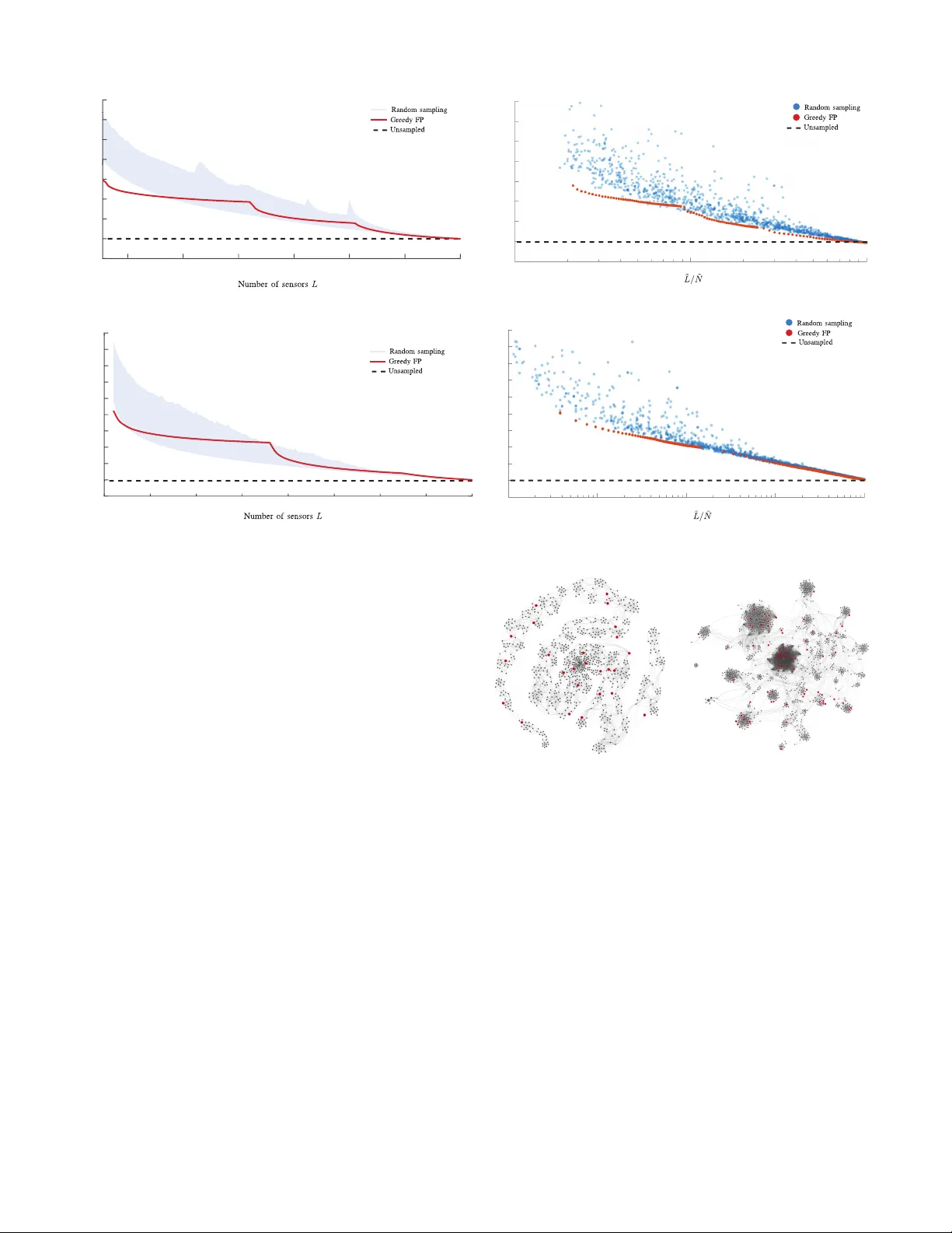
1 Sparse Sampling for In v erse Problems with T ensors Guillermo Ortiz-Jim ´ enez, Mario Coutino, Sundeep Prabhakar Chepuri, and Geert Leus Abstract —W e consider the problem of designing sparse sam- pling strategies for multidomain signals, which can be r epre- sented using tensors that admit a known multilinear decomposi- tion. W e leverage the multidomain structure of tensor signals and propose to acquire samples using a Kronecker -structur ed sensing function, thereby circumventing the curse of dimensionality . For designing such sensing functions, we develop lo w-complexity greedy algorithms based on submodular optimization methods to compute near-optimal sampling sets. W e pres ent several nu- merical examples, ranging from multi-antenna communications to graph signal processing, to validate the de veloped theory . Index T erms —Graph signal pr ocessing, multidimensional sam- pling, sparse sampling, submodular optimization, tensors I . I N T RO D U C T I O N I N many engineering and scientific applications, we fre- quently encounter large volumes of multisensor data, de- fined over multiple domains, which are complex in nature. For example, in wireless communications, received data per user may be indexed in space, time, and frequency . Simi- larly , in hyperspectral imaging, a scene measured in different wa velengths contains information from the three-dimensional spatial domain as well as the spectral domain. And also, when dealing with graph data in a recommender system, information resides on multiple domains (e.g., users, movies, music, and so on). T o process such multisensor datasets, higher -or der tensors or multiway arrays ha ve been prov en to be extremely useful. In practice, howe ver , due to limited access to sensing resources, economic or physical space limitations, it is often not possible to measure such multidomain signals using ev ery combination of sensors related to dif ferent domains. T o cope with such issues, in this work, we propose sparse sampling techniques to acquire multisensor tensor data. Sparse samplers can be designed to select a subset of measurements (e.g., spatial or temporal samples as illustrated in Fig. 1a) such that the desired inference performance is achiev ed. This subset selection problem is referred to as sparse sampling [1]. An example of this is field estimation, in which the measured field is related to the source signal of interest through a linear model. T o infer the source signal, a linear in verse problem is solved. In a resource-constrained en vironment, since many measurements cannot be taken, it is crucial to carefully select the best subset of samples from a large pool of measurements. This problem is combinatorial in nature and extremely hard to solve in general, ev en for small-sized problems. Thus, most of the research ef forts on this topic focus on finding suboptimal sampling strategies that yield good approximations of the optimal solution [1]–[10]. The authors are with the Faculty of Electrical Engineering, Mathematics and Computer Science, Delft Univ ersity of T ech- nology , The Netherlands. Email: g.ortizjimenez@student.tudelft.nl, { m.coutino;s.p.chepuri;g.j.t.leus } @tudelft.nl (a) Single domain sparse sampling (b) Unstructured multidomain sparse sampling (c) Kronecker-structured multidomain sparse sampling Fig. 1: Dif ferent sparse sensing schemes. Black (white) dots repre- sent selected (unselected) measurement locations. Blue and red lines determine dif ferent domain directions, and a purple line means that data has a single-domain structure. For signals defined over multiple domains, the dimensional- ity of the measurements gro ws much faster . An illustration of this “curse of dimensionality” is provided in Fig. 1b, wherein the measurements now have to be systematically selected from an even larger pool of measurements. T ypically used subopti- mal sensor selection strategies are not useful anymore as their complexity is too high; or simply because they need to store very large matrices that do not fit in memory (see Section III for a more detailed discussion). Usually , selecting samples arbitrarily from a multidomain signal, requires that sensors are placed densely in e very domain, which greatly increases the infrastructure costs. Hence, we propose an efficient Kr onecker - structur ed sparse sampling strategy for gathering multidomain signals that ov ercomes these issues. In Kronecker-structured sparse sampling, instead of choosing a subset of measurements from all possible combined domain locations (as in Fig. 1b), we propose to choose a subset of sensing locations from each domain and then combine them to obtain multidimensional observations (as illustrated in Fig 1c). W e will see later that taking this approach will allow us to define computationally efficient design algorithms that are useful in big data scenarios. In essence, the main question addressed in this paper is, how to choose a subset of sampling locations from each domain to sample a multidomain signal so that its reconstruction has the minimum err or? 2 I I . P R E L I M I N A R I E S In this section, we introduce the notation that will be used throughout the rest of the paper as well as some preliminary notions of tensor algebra and multilinear systems. A. Notation W e use calligraphic letters such as L to denote sets, and |L| to represent its cardinality . Upper (lower) case boldface letters such as X ( x ) are used to denote matrices (vectors). Bold calligraphic letters such as X denote tensors. ( · ) T represents transposition, ( · ) H conjugate transposition, and ( · ) † the Moore-Penrose pseudoin verse. The trace and determinant operations on matrices are represented by tr {·} and det {·} , respectiv ely . λ min { A } denotes the minimum eigen value of matrix A . W e use ⊗ to represent the Kronecker product,  to represent the Khatri-Rao or column-wise Kronecker product; and ◦ to represent the Hadamard or element-wise product between matrices. W e write the ` 2 -norm of a vector as k·k 2 and the Frobenius norm of a matrix or tensor as k·k F . W e denote the inner product between two elements of a Euclidean space as h· , ·i . The e xpectation operator is denoted by E {·} . All logarithms are considered natural. In general, we will denote the product of v ariables/sets using a tilde, i.e., ˜ N = Q R i =1 N i , or ˜ N i = N 1 × · · · × N R ; and drop the tilde to denote sums (unions), i.e., N = P R i =1 N i , or N = S R i =1 N i . Some important properties of the Kronecker and the Khatri- Rao products that will appear throughout the paper are [11]: ( A ⊗ B )( C ⊗ D ) = AC ⊗ BD ; ( A ⊗ B )( C  D ) = AC  BD ; ( A  B ) H ( A  B ) = A H A ◦ B H B ; ( A ⊗ B ) † = A † ⊗ B † ; and ( A  B ) † = ( A H A ◦ B H B ) † ( A  B ) H . B. T ensors A tensor X ∈ C N 1 ×···× N R of order R can be viewed as a discretized multidomain signal, with each of its entries index ed ov er R different domains. Using multilinear algebra two tensors X ∈ C N 1 ×···× N R and G ∈ C K 1 ×···× K R may be related by a multilinear system of equations as X = G • 1 U 1 • 2 · · · • R U R , (1) where { U i ∈ C N i × K i } R i =1 represents a set of matrices that relates the i th domain of X and the so-called cor e tensor G , and • i represents the i th mode product between a tensor and a matrix [12]; see Fig. 2a. Alternatively , vectorizing (1), we hav e x = ( U 1 ⊗ · · · ⊗ U R ) g , (2) with x = vec( X ) ∈ C ˜ N ; ˜ N = Q R i =1 N i , and g = vec( G ) ∈ C ˜ K ; ˜ K = Q R i =1 K i . When the core tensor G ∈ C K c ×···× K c is hyperdiagonal (as depicted in Fig. 2b), (2) simplifies to x = ( U 1  · · ·  U R ) g (3) with g collecting the main diagonal entries of G . Note that g has dif ferent meanings in (2) and (3), which can alw ays be inferred from the context. (a) Dense core (b) Diagonal core Fig. 2: Graphic representation of a multilinear system of equations for R = 3 . Colors represent arbitrary v alues. Such a multilinear system is commonly seen with R = 2 and X = G • 1 U 1 • 2 U 2 = U 2 G U T 1 , for instance, in image processing when relating an image to its 2-dimensional Fourier transform with G being the spatial Fourier transform of X , and U 1 and U 2 being in verse Fourier matrices related to the ro w and column spaces of the image, respectiv ely . When dealing with Fourier matrices (more generally , V andermonde matrices) with U 1 = U 2 and a diagonal tensor core, X will be a T oeplitz covariance matrix, for which the sampling sets may be designed using sparse cov ariance sensing [13], [14]. I I I . P R O B L E M M O D E L I N G W e are concerned with the design of optimal sampling strategies for an R th order tensor signal X ∈ C N 1 ×···× N R , which admits a multilinear parameterization in terms of a core tensor G ∈ C K 1 ×···× K R (dense or diagonal) of smaller dimensionality . W e assume that the set of system matrices { U i } R i =1 are perfectly kno wn, and that each of them is tall, i.e., N i > K i for i = 1 , . . . , R , and has full column rank. Sparse sampling a tensor X is equiv alent to selecting entries of x = vec( X ) . Let ˜ N denote the set of indices of x . Then, a particular sample selection is determined by a subset of selected indices L un ⊆ ˜ N such that |L un | = L un (subscript “ un ” denotes unstructured). This way , we can denote the process of sampling X as a multiplication of x by a selection matrix Θ ( L un ) ∈ { 0 , 1 } L un × ˜ N such that y = Θ ( L un ) x = Θ ( L un )( U 1 ⊗ · · · ⊗ U R ) g , (4) for a dense core [cf. (2)], and y = Θ ( L un ) x = Θ ( L un )( U 1  · · ·  U R ) g , (5) for a diagonal core [cf. (3)]. Here, y is a vector containing the L un selected entries of x indexed by the set L un . For each case, if Θ ( L un )( U 1 ⊗ · · · ⊗ U R ) and Θ ( L un )( U 1  · · ·  U R ) ha ve full column rank, then kno wing y allows to retriev e a unique least squares solution, ˆ g , as ˆ g = [ Θ ( L un )( U 1 ⊗ · · · ⊗ U R )] † y , (6) or ˆ g = [ Θ ( L un )( U 1  · · ·  U R )] † y , (7) 3 Fig. 3: Comparison between unstructured sampling and structured sampling ( R = 2 ). Black (white) cells represent zero (one) entries, and colored cells represent arbitrary numbers. depending on whether G is dense or hyperdiagonal. Next, we estimate X using either (2) or (3). In many applications, such as transmitter-recei ver placement in multiple input multiple output (MIMO) radar , it is not possible to perform sparse sampling in an unstructured manner by ignoring the underlying domains. For these applications, some unstructured sparse sample selections generally require using a dense sensor selection in each domain (as shown in Fig. 1b), which produces a significant increase in hardware cost. Also, there is no particular structure in (6) and (7) that may be exploited to compute the pseudo-in verses, thus leading to a high computational cost to estimate x . Finally , in the multidomain case, the dimensionality gro ws rather fast making it difficult to store the matrix ( U 1 ⊗ · · · ⊗ U R ) or ( U 1  · · ·  U R ) to perform row subset selection. For all these reasons, we will constrain ourselves to the case where the sampling matrix has a compatible Kronecker structure. In particular , we define a ne w sampling matrix Φ ( L ) : = Φ 1 ( L 1 ) ⊗ · · · ⊗ Φ R ( L R ) , (8) where each Φ i ( L i ) represents a selection matrix for the i th factor of X , L i ⊆ N i is the set of selected row indices from the matrix U i for i = 1 , . . . , R , and L = S R i =1 L i and L i ∩ L j = ∅ for i 6 = j. W e will use the notation |L i | = L i and |L| = P R i =1 L i = L to denote the number of selected sensors per domain and the total number of selected sensors, respectively; whereas ˜ L = L 1 × · · · × L R and ˜ L = | ˜ L| = Q R i =1 L i denote the set of sample indices and the total number of samples acquired with the abov e Kronecker -structured sampler . In order to simplify the notation, whene ver it will be clear , we will drop the e xplicit dependency of Φ i ( L i ) on the set of selected rows L i , from now on, and simply use Φ i . Imposing a Kronecker structure on the sampling scheme means that sampling can be performed independently for each domain. In the dense cor e tensor case [cf. (2)], we have y = ( Φ 1 ⊗ · · · ⊗ Φ R ) ( U 1 ⊗ · · · ⊗ U R ) g = ( Φ 1 U 1 ⊗ · · · ⊗ Φ R U R ) g = Ψ ( L ) g , (9) whereas in the diagonal cor e tensor case [cf. (3)], we ha ve y = ( Φ 1 ⊗ · · · ⊗ Φ R ) ( U 1  · · ·  U R ) g = ( Φ 1 U 1  · · ·  Φ R U R ) g = Ψ ( L ) g . (10) As in the unstructured case, whene ver (9) or (10) are ov erdetermined, using least squares, we can estimate the core ˆ g = Ψ † ( L ) y as ˆ g = h ( Φ 1 U 1 ) † ⊗ · · · ⊗ ( Φ R U R ) † i y , (11) or ˆ g = h ( Φ 1 U 1 ) H ( Φ 1 U 1 ) ◦ · · · ◦ ( Φ R U R ) H ( Φ R U R ) i † × h ( Φ 1 U 1 ) H  · · ·  ( Φ R U R ) H i y , (12) and then reconstruct ˆ x using (2) or (3), respecti vely . Compar- ing (11) and (12) to (6) and (7) we can see that lev eraging the Kronecker structure of the proposed sampling scheme allows to greatly reduce the computational complexity of the least-squares problem, as the pseudoin verses in (11) and (12) are taken on matrices of a much smaller dimensionality than in (6) and (7). An illustration of the comparison between unstructured sparse sensing and Kronecker-structured sparse sensing is shown in Fig. 3 for R = 2 . Suppose the measurements collected in y are perturbed by zero-mean white Gaussian noise with unit variance, then the least-squares solution has the in verse error covariance or the Fisher information matrix T ( L ) = E { ( g − ˆ g )( g − ˆ g ) H } = 4 Ψ H ( L ) Ψ ( L ) that determines the quality of the estimators ˆ g . Therefore, we can use scalar functions of T ( L ) as a figure of merit to propose the sparse tensor sampling problem optimize L 1 ,..., L R f { T ( L ) } s. to R X i =1 |L i | = L, L = R [ i =1 L i , (13) where with “optimize” we mean either “maximize” or “min- imize” depending on the choice of the scalar function f {·} . Solving (13) is not trivial due to the cardinality constraints. Therefore, in the follo wing, we will propose tight surrogates for typically used scalar performance metrics f {·} in design of experiments with which the abov e discrete optimization problem can be solved ef ficiently and near optimally . Note that the cardinality constraint in (13) restricts the total number of selected sensors to L , without imposing any constraint on the total number of gathered samples ˜ L . Although the maximum number of samples can be constrained using the constraint P R i =1 log |L i | ≤ ˜ L , the resulting near- optimal solv ers are computationally intense with a comple xity of about O ( N 5 ) [15], [16]. Such heuristics are not suitable for the large-scale scenarios of interest. A. Prior art Choosing the best subset of measurements from a large set of candidate sensing locations has received a lot of attention, particularly for R = 1 , usually under the name of sensor selection/placement, which also is more generally referred to as sparse sensing [1]. T ypically sparse sensing design is posed as a discrete optimization problem that finds the best sampling subset by optimizing a scalar function of the error cov ariance matrix. Some of the popular choices are, to minimize the mean squared error (MSE): f { T ( L ) } := tr  T − 1  or the frame potential: f { T ( L ) } := tr n T H T o , or to maximize f { T ( L ) } := λ min { T } or f { T ( L ) } := log det { T } . In this work, we will focus on the frame potential criterium as we will show later that this metric leads to very efficient sampler designs. Depending on the strategy used to solve the optimization problem (13) we can classify the prior art in two categories: solvers based on con vex optimization, and greedy methods that lev erage submodularity . In the former category , [2] and [8] present sev eral con vex relaxations of the sparse sensing problem for different optimality criteria for inv erse problems with linear and non-linear models, respectiv ely . In particular , due to the Boolean nature of the sensor selection problem (i.e., a sensor is either selected or not), its related optimization problem is not conv ex. Howe ver , these constraints and the constraint on the number of selected sensors can be relaxed, and once the relaxed conv ex problem is solved, a thresholding heuristic (deterministic or randomized) can be used to recov er a Boolean solution. Despite its good performance, the com- plexity of con ve x optimization solvers is rather high (cubic with the dimensionality of the signal). Therefore, the use of con vex optimization approaches to solve the sparse sensing problem in large-scale scenarios, such as the sparse tensor sampling problem, gets ev en more computationally intense. For high-dimensional scenarios, greedy methods (algo- rithms that select one sensor at a time) are more useful. A greedy algorithm scales linearly with the number of sensors, and if one can prov e submodularity of the objecti ve function, its solution has a multiplicative near -optimality guarantee [17]. Sev eral authors have followed this strategy and have prov ed submodularity of different optimality criteria such as D - optimality [4], mutual information [3], and frame potential [5]. All of them for the case R = 1 . Besides parameter estimation, sparse sensing has also been studied for other common signal processing tasks, like detec- tion [6], [9] and filtering [7], [10]. In a different context, the extension of Compressed Sensing (CS) to multidomain signals has been extensi vely studied [18]–[21]. CS is many times seen as a complementary sampling frame work to sparse sensing [1], wherein CS the focus is on recov ering a sparse signal rather than on designing a sparse measurement space. B. Our contributions In this paper , we extend the sparse sampling framew ork to multilinear in verse pr oblems . W e refer to it as “sparse tensor sampling”. W e focus on two particular cases, depending on the structure of the core tensor G : • Dense cor e : Whenev er the core tensor is non-diagonal, sampling is performed based on (9). W e will see that to ensure identifiability of the system, we need to select more entries in each domain than the rank of its corre- sponding system matrix, i.e., as a necessary condition we require L ≥ P R i =1 K i = K sensors, where { K i } R i =1 are the dimensions of the core tensor G . • Diagonal cor e : Whenever the core tensor is diagonal, sampling is performed based on (10). The use of the Khatri-Rao product allows for higher compression. In particular , under mild conditions on the entries of the factor matrices, we can guarantee identifiability of the sampled equations using L ≥ K c + R − 1 sensors, where K c is the length of the edges of the hypercubic core G . For both the cases, we propose efficient greedy algorithms to compute a near-optimal sampling set. C. P aper outline The remainder of the paper is organized as follows. In Sections IV and V, we develop solv ers for the sparse tensor sampling problem with dense and diagonal core tensors, respectiv ely . In Section VI, we provide a few examples to illustrate the dev eloped framew ork. Finally , we conclude this paper by summarizing the results in Section VII. I V . D E N S E C O R E S A M P L I N G In this section, we focus on the most general situation when G is an unstructured dense tensor . Our objectiv e is to design the sampling sets {L i } R i =1 by solving the discrete optimization problem (13). W e formulate the sparse tensor sampling problem using the frame potential as a performance measure. Follo wing the same rationale as in [5], but for multidomain signals, we will 5 argue that the frame potential is a tight surrogate of the MSE. By doing so, we will see that when we impose a Kronecker structure on the sampling scheme, as in (8), the frame potential of Ψ can be factorized in terms of the frame potential of the different domain factors. This allows us to propose a lo w complexity algorithm for sampling tensor data. Throughout this section, we will use tools from submodular optimization theory . Hence, we will start by introducing the main concepts related to submodularity in the next subsection. A. Submodular optimization Submodularity is a notion based on the law of diminishing returns [22] that is useful to obtain heuristic algorithms with near-optimality guarantees for cardinality-constrained discrete optimization problems. More precisely , submodularity is for- mally defined as follows. Definition 1 (Submodular function [22]) . A set function f : 2 N → R defined over the subsets of N is submodular if, for every X ⊆ N and x, y ∈ N \ X , we have f ( X ∪ { x } ) − f ( X ) ≥ f ( X ∪ { x, y } ) − f ( X ∪ { y } ) . A function f is said to be supermodular if − f is submodular . Besides submodularity , many near-optimality theorems in discrete optimization require functions to be also monotone non-decreasing, and normalized. Definition 2 (Monotonicity) . A set function f : 2 N → R is monotone non-decr easing if, for every X ⊆ N , f ( X ∪ { x } ) ≥ f ( X ) ∀ x ∈ N \ X Definition 3 (Normalization) . A set function f : 2 N → R is normalized if f ( ∅ ) = 0 . In submodular optimization, matroids are generally used to impose constraints on an optimization, such as the ones in (13). A matroid generalizes the concept of linear independence in algebra to sets. Formally , a matroid is defined as follows. Definition 4 (Matroid [23]) . A finite matr oid M is a pair ( N , I ) , where N is a finite set and I is a family of subsets of N that satisfies: 1) The empty set is independent, i.e ., ∅ ∈ I ; 2) F or e very X ⊆ Y ⊆ N , if Y ∈ I , then X ∈ I ; and 3) F or every X , Y ⊆ N with |Y | > |X | and X , Y ∈ I ther e exists one x ∈ Y \ X such that X ∪ { x } ∈ I . In this paper we will deal with the follo wing types of matroids. Example 1 (Uniform matroid [23]) . The subsets of N with at most K elements form a uniform matr oid M u = ( N , I u ) with I u = {X ⊆ N : |X | ≤ K } . Example 2 (Partition matroid [23]) . If {N i } R i =1 form a partition of N = S R i =1 N i then M p = ( N , I p ) with I p = {X ⊆ N : |X ∩ N i | ≤ K i i = 1 , . . . , R } defines a partition matr oid. Example 3 (Truncated partition matroid [23]) . The intersec- tion of a uniform matr oid M u = ( N , I u ) and a partition Algorithm 1 Greedy maximization subject to T matroid constraints Require: X = ∅ , K , {I i } T i =1 1: for k ← 1 to K 2: s ? = arg max s / ∈X { f ( X ∪ { s } ) : X ∪ { s } ∈ T T i =1 I i } 3: X ← X ∪ { s ? } 4: end 5: retur n X matr oid M p = ( N , I p ) defines a truncated partition matr oid M t = ( N , I p ∩ I u ) . The matroid-constrained submodular optimization problem maximize X ⊆N f ( X ) subject to X ∈ T \ i =1 I i (14) can be solved near optimally using Algorithm 1. This result is formally stated in the following theorem. Theorem 1 (Matroid-constrained submodular maximization [24]) . Let f : 2 N → R be a monotone non-decr easing, normalized, submodular set function, and {M i = ( N , I i ) } T i =1 be a set of matr oids defined over N . Furthermor e, let X ? denote the optimal solution of (14) , and let X gr eedy be the solution obtained by Algorithm 1. Then f ( X gr eedy ) ≥ 1 T + 1 f ( X ? ) . B. Gr eedy method The frame potential [25] of the matrix Ψ is defined as the trace of the Grammian matrix FP ( Ψ ) : = tr n T H T o with T = Ψ H Ψ . The frame potential can be related to the MSE, MSE( Ψ ( L )) = tr  T − 1 ( L )  , using [5] c 1 FP ( Ψ ( L )) λ 2 max { T ( L ) } ≤ MSE( Ψ ( L )) ≤ c 2 FP ( Ψ ( L )) λ 2 min { T ( L ) } , (15) where c 1 , and c 2 are constants that depend the data model. From the above bound, it is clear that by minimizing the frame potential of Ψ one can minimize the MSE, which is otherwise difficult to minimize as it is neither con ve x, nor submodular . The frame potential of Ψ ( L ) : = Ψ 1 ( L 1 ) ⊗ · · · ⊗ Ψ R ( L R ) can be e xpressed as the frame potential of its factors Ψ i ( L i ) : = Φ i ( L i ) U i . T o show this, recall the definition of the frame potential as FP ( Ψ ( L )) = tr n T H ( L ) T ( L ) o = tr n T H 1 T 1 ⊗ · · · ⊗ T H R T R o , (16) where T i = Ψ H i Ψ i . Now , using the fact that for any two matrices A ∈ C K A × K A and B ∈ C K B × K B we have tr { A ⊗ B } = tr { A } tr { B } , we can expand (16) as FP ( Ψ ( L )) = R Y i =1 tr n T H i T i o = R Y i =1 FP ( Ψ i ( L i )) . 6 For brevity , we will write the above expression alternatively as an explicit function of the selection sets L i : F ( L ) : = FP ( Ψ ( L )) = R Y i =1 F i ( L i ) : = R Y i =1 FP ( Ψ i ( L i )) (17) Expression (17) shows again the advantage of working with a Kronecker -structured sampler: instead of computing ev ery cross-product between the columns of Ψ to compute the frame potential, we can arrive to the same value using the frame potential of { Ψ i } R i =1 . 1) Submodularity of F ( L ) : Function F ( L ) as defined in (17) does not directly meet the conditions [cf. Theorem 1] required for near optimality of the greedy heuristic, but it can be modified slightly to satisfy them. In this sense, we define the function G : 2 N → R on the subsets of N as G ( S ) : = F ( N ) − F ( N \ S ) (18) where recall that F ( N ) = Q R i =1 F i ( N i ) , F ( N \ S ) = Q R i =1 F i ( N i \ S i ) , and S = S R i =1 S i , S i ∩ S j = ∅ for i 6 = j . Therefore, {S i } R i =1 form a partition of S . It is clear that if we make the change of v ariables from L to S maximizing G over S is the same as minimizing the frame potential over L . Ho wev er, working with the complement set results in a set function that is submodular and monotone non- decreasing, as sho wn in the next theorem. Consequently , G satisfies the conditions of the near-optimality theorems. Theorem 2. The set function G ( S ) defined in (18) is a normalized, monotone non-decreasing , submodular function for all subsets of N = S R i =1 N i . Pr oof. See Appendix A. W ith this result we can now claim near-optimality of the greedy algorithm that solves the cardinality constrained maximization of G ( S ) . Ho wev er , as we said, minimizing the frame potential only makes sense as long as (15) is tight. In particular , whenev er T ( L ) is singular we know that the MSE is infinity , and hence (15) is meaningless. F or this reason, next to the cardinality constraint in (13) that limits the total number of sensors, we need to ensure that Ψ ( L ) has full column rank, i.e., L i ≥ K i for i = 1 , . . . , R . In terms of S , this is equiv alent to |S i | = |N i \ L i | ≤ N i − K i i = 1 , . . . , R, (19) where this set of constraints forms a partition matroid M p = ( N , I p ) [cf. Example 2 from Definition 4]. Hence, we can introduce the following submodular optimization problem as surrogate for the minimization of the frame potential maximize S ⊆N G ( S ) s. to S ∈ I u ∩ I p (20) with I u = {A ⊆ N : |A| ≤ N − L } and I p = {A ⊆ N : |A ∩ N i | ≤ N i − K i i = 1 , . . . , R } . Theorem 1 gives, therefore, all the ingredients to assess the near-optimality of Algorithm 1 applied on (20), for which the results are particularized as the following corollary . Corollary 1. The gr eedy solution S gr eedy to (20) obtained from Algorithm 1) is 1 / 2 -near-optimal, i.e., G ( S gr eedy ) ≥ 1 2 G ( S ? ) . Pr oof. Follows from Theorem 1, and since (20) has T = 1 (truncated-partition) matroid constraint. Next, we compute an explicit bound with respect to the frame potential of Ψ , which is the objecti ve function we initially wanted to minimize. This bound is giv en in the following theorem. Theorem 3. The greedy solution L gr eedy to (20) obtained fr om Algorithm 1 is near optimal with respect to the frame potential as F ( L gr eedy ) ≤ γ F ( L ? ) with γ = 1 2 K L 2 min Q R i =1 F i ( N i ) + 1 ! , and L min = min i ∈L k u i k 2 2 , be- ing u i the i th r ow of ( U 1 ⊗ · · · ⊗ U R ) . Pr oof. Obtained similar to the bound in [5], but specialized for (17) and 1/2-near-optimality; see [26] for details. As with the R = 1 case in [5], γ is heavily influenced by the frame potential of ( U 1 ⊗ · · · ⊗ U R ) . Specifically , approximation gets tighter when F ( N ) is small or the core tensor dimensionality decreases. 2) Computational complexity: The running time of Al- gorithm 1 applied to solve (20) can greatly be reduced by precomputing the inner products between the rows of every U i before starting the iterations. This has a complexity of O ( N 2 i K i ) for each domain. Once these inner products are computed, in each iteration we need to find R times the max- imum ov er O ( N i ) elements. Since we run N − L iterations, the complexity of all iterations is O ( N 2 max ) , with N max = max i N i . Therefore, the total computational complexity of the greedy method is O ( N 2 max K max ) with K max = max i K i . 3) Practical considerations: Due to the characteristics of the greedy iterations, the algorithm tends to give solutions with a very unbalanced cardinality . In particular , for most situations, the algorithm chooses one of the domains in the first few iterations and empties that set till it hits the identifiability constraint of that domain. Then, it proceeds to another domain and empties it as well, and so on. This is due to the objecti ve function, which is a product of smaller objectives. Indeed, if we are asked to minimize a product of two elements by subtracting a v alue from them, it is generally better to subtract from the smallest element. Hence, if this minimization is performed multiple times we will tend to remov e alw ays from the same element. The consequences of this beha vior are twofold. On the one hand, this greedy method tends to giv e a sensor placement that yields a very small number of samples ˜ L , as we will also see in the simulations. Therefore, when comparing this method to other sensor selection schemes that produce solutions with a larger ˜ L it generally ranks worse in MSE for a giv en L . On the other hand, the solution of this scheme tends to be tight on the identifiability constraints for most of the domains, thus hampering the performance on those domains. This implication, ho wever , has a simple solution. By introducing a small slack v ariable α i > 0 to the constraints, we can obtain 7 a sensor selection which is not tight on the constraints. This amounts to solving the problem maximize S ⊆N G ( S ) (21) s. to |S | = N − L, |S ∩ N i | ≤ N i − K i − α i , i = 1 , . . . , R. T uning { α i } R i =1 allows to regularize the tradeoff between compression and accuracy of the greedy solution. W e conclude this section with a remark on an alternativ e performance measure. Remark. As a alternative performance measur e, one can think on maximizing the set function log det { T ( L ) } . Although this set function can be shown to be submodular over all subsets of N [26], the r elated greedy algorithm cannot be constrained to always result in an identifiable system after subsampling. Thus, its applicability is mor e limited than the frame potential formulation; see [26] for a more detailed discussion. V . D I AG O N A L C O R E S A M P L I N G So far , we have focused on the case when G is dense and has no particular structure. In that case, we have seen that we require at least P R i =1 K i sensors to recov er our signal with a finite MSE. In many cases of interest, G admits a structure. In particular , in this section, we inv estigate the case when G is a diagonal tensor . Under some mild conditions on the entries of { U } R i =1 , we can lev erage the structure of G to further increase the compression. As before, we dev elop an efficient and near-optimal greedy algorithm based on minimizing the frame potential to design the sampling set. A. Identifiability conditions In contrast to the dense core case, the number of unknowns in a multilinear system of equations with a diagonal core does not increase with the tensor order , whereas for a dense core it grows exponentially . This means that when sampling signals with a diagonal core decomposition, one can expect a stronger compression. T o derive the identifiability conditions for (10), we present the result from [27] as the following theorem. Theorem 4 (Rank of Khatri-Rao product [27]) . Let A ∈ C N × K and B ∈ C M × K be two matrices with no all-zer o column. Then, rank( A  B ) ≥ max { rank( A ) , rank( B ) } . Based on the above theorem, we can giv e the following sufficient conditions for identifiability of the system (10). Corollary 2. Let z i denote the maximum number of zer o entries in any column of U i . If for every Ψ i ( L i ) we have |L i | > z i , and there is at least one Ψ j with rank( Ψ j ) = K c , then Ψ ( L ) has full column rank. Pr oof. Selecting L i > z i rows from each U i ensures that no Ψ i will have an all-zero column. Then, if for at least one Ψ j we hav e rank( Ψ j ) = K c , then due to Theorem 4 we have rank( Ψ ( L )) ≥ max i =1 ,...,R { rank( Ψ i ) } = max  rank( Ψ j ) , max i 6 = j { rank( Ψ j ) }  = K c . Therefore, in order to guarantee identifiability we need to select L j ≥ max { K c , z j + 1 } ro ws from any factor matrix j , and L i ≥ max { 1 , z i + 1 } from the other f actors with i 6 = j . In many scenarios, we usually hav e { z i = 0 } R i =1 since no entry in { U i } R i =1 will exactly be zero. In those situations we will require to select at least L = P R i =1 L i ≥ K c + R − 1 elements. B. Gr eedy method As we did for the case with a dense core, we start by finding an expression for the frame potential of a Khatri-Rao product in terms of its factors. The Grammian matrix T ( L ) of a diagonal core tensor decomposition has the form T = Ψ H Ψ = ( Ψ 1  · · ·  Ψ R ) H ( Ψ 1  · · ·  Ψ R ) = Ψ H 1 Ψ 1 ◦ · · · ◦ Ψ H R Ψ R = T 1 ◦ · · · ◦ T R . Using this expression, the frame potential of a Khatri-Rao product becomes FP ( Ψ ) = tr n T H T o = k T k 2 F = k T 1 ◦ · · · ◦ T R k 2 F . (22) For brevity , we will denote the frame potential as an explicit function of the selected set as P ( L ) : = FP ( Ψ ( L )) = k T 1 ( L 1 ) ◦ · · · ◦ T R ( L R ) k 2 F . (23) Unlike in the dense core case, the frame potential of a Khatri-Rao product cannot be separated in terms of the frame potential of its factors. Instead, (22) decomposes the frame potential using the Hadamard product of the Grammian of the factors. 1) Submodularity of P ( L ) : Since P ( L ) does not directly satisfy the conditions [cf. Theorem 1] required for near opti- mality of the greedy heuristic, we propose using the follo wing set function Q : 2 N → R as a surrogate for the frame potential Q ( S ) : = P ( N ) − P ( N \ S ) (24) with P ( N ) = k T 1 ( N 1 ) ◦ · · · ◦ T r ( N r ) k 2 F and P ( N \ S ) = k T 1 ( N 1 \ S 1 ) ◦ · · · ◦ T R ( N R \ S R ) k 2 F . Theorem 5. The set function Q ( S ) defined in (24) is a normalized, monotone non-decreasing , submodular function for all subsets of N = S R i =1 N i . Pr oof. See Appendix B. Using Q and imposing the identifiability constraints defined in Section V -A we can write the related optimization problem for the minimization of the frame potential as maximize S ⊆N Q ( S ) s. to S ∈ I u ∩ I p (25) 8 where I u = {A ⊆ N : |S | ≤ N − L } and I p = {A ⊆ N : |A ∩ N i | ≤ β i i = 1 , . . . , R } with β j = N j − max { K c , z j } and β i = N i − max { 1 , z i + 1 } for i 6 = j . Here, the choice of j is arbitrary , and can be set depending on the application. For example, with some space-time signals it is more costly to sample space than time, and, in those cases, j is generally chosen for the temporal domain. This is a submodular maximization problem with a trun- cated partition matroid constraint [cf. Example 2 from Def- inition 4]. Thus, from Theorem 1, we know that greedy maximization of (25) using Algorithm 1 has a multiplicati ve near-optimal guarantee. Corollary 3. The gr eedy solution S gr eedy to (25) obtained using Algorithm 1 is 1 / 2 -near-optimal, i.e., Q ( S gr eedy ) ≥ 1 2 Q ( S ? ) . Her e, S ? denotes the optimal solution of (25) . Similar to the dense core case, we can also pro vide a bound on the near-optimality of of the greedy solution with respect to the frame potential. Theorem 6. The solution set L gr eedy = N \ S gr eedy ob- tained fr om Algorithm 1 is near optimal with respect to the frame potential as P ( L gr eedy ) ≤ γ P ( L ? ) , with γ = 0 . 5  k T 1 ( N 1 ) ◦ · · · ◦ T R ( N R ) k 2 F K L − 2 min + 1  and L ? = N \ S ? . Pr oof. Based on the proof of Theorem 3. The bound is obtained using (22) instead of (17) in the deriv ation. 2) Computational complexity: The computational complex- ity of the greedy method is now gov erned by the comple xity of computing the Grammian matrices T i . This can greatly be improv ed if before starting the iterations, one precomputes all the outer products in { T i } R i =1 . Doing this has a computational complexity of O ( N max K 2 c ) . Then, in ev ery iteration, the ev al- uation of P ( L ) would only cost O ( RK 2 c ) operations. Further , because in ev ery iteration we need to query O ( N i ) elements on each domain, and we run the algorithm for N − L iterations, the total time comple xity of the iterations is O ( RN 2 max K 2 c ) . This term dominates over the complexity of the precomputations, and thus can be treated as the worst case complexity of the greedy method. 3) Practical considerations: The proposed scheme suffers from the same issues as in the dense core case. Namely , it tends to empty the domains sequentially , thus producing solutions which are tight on the identifiability constraints. Ne vertheless, as we indicated for the dense core, the drop in performance associated with the proximity of the solutions to the constraints can be reduced by giving some slack to the constraints. V I . N U M E R I C A L R E S U LT S In this section 1 , we will illustrate the de veloped framew ork through several examples. First, we will show some results obtained on synthetic datasets to compare the performance of the dif ferent near -optimal algorithms. Then, we will focus on large-scale real-world examples related to (i) graph signal 1 The code to reproduce these experiments can be found at https://gitlab .com/gortizji/sparse tensor sensing. processing: sampling pr oduct graphs for active learning in r ecommender systems , and (ii) array processing for wireless communications: multiuser sour ce separation , to show the benefits of the dev eloped framew ork. A. Synthetic example 1) Dense core: W e compare the performance in terms of the theoretical MSE of our proposed greedy algorithm (henceforth referred to as greedy-FP) to a random sampling scheme based on randomly selecting rows of U i such that the resulting subset of samples also have a Kronecker structure. Only those selections that satisfy the identifiability constraints in (19) are considered valid. W e note that the time complexity of ev aluating M times the MSE for a Kronecker-structured sampler is O ( M N 2 max K max ) . For this reason, using many realizations (say , a large number M ) of random sampling to obtain a good sparse sampler is computationally intense. T o perform this comparison, we draw M = 100 realizations of three random Gaussian matrices { U i ∈ R N i × K i } R =3 i =1 with dimensions N 1 = 50 , N 2 = 60 , and N 3 = 70 . For each of these models, we solve (20) for different number of sensors L using greedy-FP . W e also compute M = 100 realizations of random sampling for each L . Fig. 4 sho ws the results of these experiments. The plot on the left shows the performance averaged over the different models against the number of sensors, wherein the blue shaded area represents the 10-90 percentile average interv al of the random sampling scheme. The performance v alues, in dB scale, are normalized by the v alue of the unsampled MSE. Because the estimation performance is heavily influenced by its related number of samples ˜ L , and noting the fact that a value of L may lead to different ˜ L , we also present, in the plot on the right side of Fig. 4, the performance comparison for one model realization against the relati ve number of samples ˜ L/ ˜ N so that dif ferences in the informativ e quality of the selections are highlighted. The plots in Fig. 4 illustrate some important features of the proposed sparse sampling method. When comparing the performance against the number of sensors, we see that there are areas where greedy-FP performs as well as random sampling. Howe ver , when comparing the same results against the number of samples we see that greedy-FP consistently performs better than random sampling. The reason for this disparity is due to characteristics of greedy-FP that we intro- duced in Section IV -B. Namely , the tendency of greedy-FP to produce sampling sets with the minimum number of samples. On the other hand, the performance curve of greedy-FP shows three b umps (recall that we use R = 3 ). Again, this is a consequence of greedy-FP trying to meet the identifiability constraints in (20) with equality . As we increase L , the solutions of greedy-FP increase in cardinality by adding more elements to a single domain until the constraints are met, and then proceed to the next domain. The b umps in Fig. 4 correspond precisely to these instances. 2) Diagonal core: W e perform the same e xperiment for the diagonal core case. The results are sho wn in Fig. 5. Again we see that the proposed algorithm outperforms random sampling, especially when collecting just a fe w samples. Furthermore, 9 60 80 100 120 140 160 180 MSE (dB) 1% 10% 100% -10 0 10 20 30 40 50 60 70 MSE (dB) -10 0 10 20 30 40 50 60 70 Fig. 4: Dense core with R = 3 , N 1 = 50 , N 2 = 60 , N 3 = 70 , K 1 = 10 , K 2 = 20 , K 3 = 15 , and α 1 = α 2 = α 3 = 2 . 20 40 60 80 100 120 140 160 180 MSE (dB) -10 0 10 20 30 40 50 60 70 80 90 MSE (dB) -10 0 10 20 30 40 50 60 70 80 90 1% 10% 100% 0.1% 0.01% Fig. 5: Diagonal core with R = 3 with N 1 = 50 , N 2 = 60 , N 3 = 70 , K c = 20 , β 1 = β 2 = 1 , and β 3 = 20 . as happened in the dense core case, the performance curve of greedy-FP follows a stairway shape. B. Active learning for r ecommender systems Current recommendation algorithms seek solving an estima- tion problem of the form: giv en the past recorded preferences of a set of users, what is the rating that these would give to a set of products? In this paper , in contrast, we focus on the data acquisition phase of the recommender system, which is also referred to as activ e learning/sampling. In particular , we claim that by carefully designing which users to poll and on which items, we can obtain an estimation performance on par with the state-of-the-art methods, but using only a fraction of the data that current methods require, and using a simple least-squares estimator . W e sho wcase this idea on the MovieLens 100 k dataset [28] that contains partial ratings of N 1 = 943 users over N 2 = 1682 movies which are stored in a second-order tensor X ∈ R N 1 × N 2 . At this point, we emphasize the need for our proposed framework, since it is obvious that designing an unstructured sampling set with about 1.5 million candidate locations is unfeasible with current computing resources. A model of X in the form of (1) can be obtained by viewing X as a signal that lives on a graph. In particular, the first two modes of X can be viewed as a signal defined on the Cartesian product of a user and movie graph, respectiv ely . These two graphs, shown in Fig. 6, are provided in the dataset and are two 10-nearest-neighbors graphs created based on the user and movie features. Based on the recent advances in graph signal processing (GSP) [29], [30], X can be decomposed as X = X f • 1 (a) User graph (b) Movie graph Fig. 6: User and movie networks. The red (black) dots represent the observ ed (unobserved) vertices. V isualization obtained using Gephi [33]. V 1 • 2 V 2 . Here, V 1 ∈ R N 1 × N 1 and V 2 ∈ R N 2 × N 2 are the eigenbases of the Laplacians of the user and movie graphs, respectiv ely , and X f ∈ C N 1 × N 2 is the so-called graph spectrum of X [29], [30]. Suppose the energy of the spectrum of X is concentrated in the first few K 1 and K 2 columns of V 1 and V 2 , respectiv ely , then X admits a low-dimensional representation, or X is said to be smooth or bandlimited with respect to the underlying graph [30]. This property has been exploited in [31], [32] to impute the missing entries in X . In contrast, we propose a scheme for sampling and reconstruction of signals defined on product graphs. In our e xperiments, we set K 1 = K 2 = 20 , and obtain the decomposition X = G • 1 U 1 • 2 U 2 , where U 1 ∈ C N 1 × K 1 and U 2 ∈ C N 2 × K 1 consist of the first K 1 and K 2 columns of V 1 and V 2 , respectiv ely; and G = X (1 : K 1 , 1 : K 2 ) . For the greedy algorithm we use L = 100 and α 1 = α 2 = 5 , resulting in a selection of L 1 = 25 users and L 2 = 75 movies, 10 Method Number of samples RMSE GMC [31] 80,000 0.996 GRALS [34] 80,000 0.945 sRGCNN [35] 80,000 0.929 GC-MC [36] 80,000 0.905 Our method 1,875 0.9347 T ABLE I: Performance on MovieLens 100 k . Baseline scores are taken from [36]. i.e., a total of 1875 vertices in the product graph. Fig. 6, sho ws the sampled users and movies, i.e., users to be probed for movie ratings. The user graph [cf. Fig. 6a] is made out of small clusters connected in a chain-like structure, resulting in a uniformly spread distribution of observed vertices. On the other hand, the movies graph [cf. Fig. 6b] is made out of a few big and small clusters. Hence, the proposed activ e querying scheme assigns more observations to the bigger clusters and fewer observations to the smaller ones. T o ev aluate the performance of our algorithm, we compute the RMSE of the estimated data using the test mask provided by the dataset. Nev ertheless, since our activ e query method requires access to ground truth data (i.e., we need access to the samples at locations suggested by the greedy algorithm) which is not provided in the dataset, we use GRALS [34] to complete the matrix, and use its estimates when required. A comparison of our algorithm to the performance of the state-of-the-art methods run on the same dataset is sho wn in T able I. In light of these results, it is clear that a proper design of the sampling set allows to obtain top performance with significantly fewer ratings, i.e., about an order of magnitude, and using a much simpler non-iterativ e estimator . C. Multiuser sour ce separation In multiple-input multiple-output (MIMO) communications [37], the use of rectangular arrays [38] allows to separate signals coming from different azimuth and elev ation angles, and it is common that users transmit data using different spreading codes to reduce the interference from other sources. Reducing hardware complexity by minimizing the number of antennas and samples to be processed is an important concern in the design of MIMO receivers. This design can be seen as a particular instance of sparse tensor sampling. W e consider a scenario with K c users located at different an- gles of azimuth ( φ ) and ele vation ( θ ) transmitting using unique spreading sequences of length N 3 . The recei ver consists of a uniform rectangular array (URA) with antennas located on a N 1 × N 2 grid. Each time instant, e very antenna recei ves [38] x ( r , l , m, n ) = K c X k =1 s k ( r ) c k ( l ) e j 2 πn ∆ x sin θ k e j 2 πm ∆ y sin φ k + w ( r , l, m, n ) , where s k ( r ) the symbol transmitted by user k in the r th symbol period; c k ( l ) the l th sample of the spreading sequence of the k th user; ∆ x and ∆ y the antenna separations in wave- lengths of the URA in the x and y dimensions, respectiv ely; MSE (dB) SNR (dB) 20 40 0 -20 -40 -60 -80 20 10 0 -20 -10 -30 -40 -50 Fig. 7: MSE of symbol reconstruction. N 1 = 50 , N 2 = 60 , N 3 = 100 , and L = 15 . and φ k and θ k the azimuth and elev ation coordinates of user k , respecti vely; and where w ( r , l , m, n ) represents an additi ve white Gaussian noise term with zero mean and variance σ 2 . For the r -th symbol period, all these signals can be collected in a 3rd-order tensor X ( r ) ∈ C N 1 × N 2 × N 3 that can be decomposed as X ( r ) = S ( r ) • 1 U 1 • 2 U 2 • 3 U 3 + W ( r ) where U 1 ∈ C N 1 × K c and U 2 ∈ C N 2 × K c are the array re- sponses for the x and y directions, respecti vely; U 3 ∈ C N 3 × K c contains the spreading sequences of all users in its columns; and S ( r ) ∈ C K c × K c × K c is a diagonal tensor that stores the symbols of all users for the r th symbol period on its diagonal. W e simulate this setup using K c = 10 users that transmit BPSK symbols with different random powers and that are equispaced in azimuth and elev ation. W e use a rectangular array with N 1 = 50 and N 2 = 60 for the ground set locations of the antennas, and binary random spreading sequences of length N 3 = 100 . W ith these parameters, each X ( r ) has 300 , 000 entries. W e generate many realizations of these signals for dif ferent le vels of signal-to-noise ratio (SNR) and sample the resulting tensors using the greedy algorithm for the diagonal core case with L = 15 , resulting in a relati ve number of samples of 0 . 048% . The results are depicted in Fig. 7, where the blue shaded area represents the MSE obtained with the best and worst random samplers. As expected, the MSE of the reconstruction decreases exponentially with the SNR. For a given MSE, achieving maximum compression requires transmitting with a higher SNR of about 30dB than the one needed for no compression. Besides, we see that our proposed greedy algorithm consistently performs as well as the best random sampling scheme. V I I . C O N C L U S I O N S In this paper, we presented the design of sparse samplers for in verse problems with tensors. W e have seen that by using samplers with a Kronecker structure we can ov ercome the curse of dimensionality , and design efficient subsampling schemes that guarantee a good performance for the recon- struction of multidomain tensor signals. W e presented sparse sampling design methods for cases in which the multidomain signals can be decomposed using a multilinear model with a dense core or a diagonal core. For both cases, we hav e pro- vided a near-optimal greedy algorithm based on submodular optimization methods to compute the sampling sets. 11 A P P E N D I X A. Pr oof of Theorem 2 In order to simplify the deriv ations, let us introduce the notation ¯ F i ( S i ) = F i ( N i \ S i ) , so that G ( S ) can also be written G ( S ) : = R Y i =1 F i ( N i ) − R Y i =1 ¯ F i ( S i ) . (26) From (26) it is e vident that G ( ∅ ) = 0 . Thus, pro ving that G is normalized. T o prove monotonicity , recall that the single domain frame potential terms F i ( L i ) are all non-negativ e, monotone non-decreasing functions for all L i ⊆ N i [5]. Therefore, ¯ F i ( S i ) = F i ( N \ S i ) will be non-negati ve, but monotone non-increasing. Let S ⊆ N and x ∈ N \ S . W ithout loss of generality , let us assume x ∈ N i . Then, we hav e G ( S ∪ { x } ) = R Y i =1 F i ( N i ) − ¯ F i ( S i ∪ { x } ) Y j 6 = i ¯ F j ( S j ) , G ( S ) = R Y i =1 F i ( N i ) − ¯ F i ( S i ) Y j 6 = i ¯ F j ( S j ) . Now , since ¯ F i ( S i ) ≥ ¯ F i ( S i ∪{ x } ) , we kno w that G ( S ∪{ x } ) ≥ G ( S ) . Hence, G ( S ) is monotone non-decreasing. T o prov e submodularity , recall that ev ery F i ( L i ) is su- permodular [5]. As taking the complement preserves (su- per)submodularity , ¯ F i ( L i ) = F i ( N i \ L i ) is also supermodular . Let S = S R i =1 A i , with A i ⊆ N i for i = 1 , . . . , R , such that {A i } R i =1 , forms a partition of S . Now , recall from Definition 1 that for G to be submodular we require that ∀ x, y ∈ N \ S G ( S ∪ { x } ) − G ( S ) ≥ G ( S ∪ { x, y } ) − G ( S ∪ { y } ) . (27) As the ground set is no w partitioned into the union of several ground sets, there are two possible ways the elements x and y can be selected. Either the y both belong to the same domain, or they belong to dif ferent domains. W e next prove that (27) is satisfied for the aforementioned both cases. Suppose x, y ∈ N i , then (27) can be dev eloped as ¯ F i ( A i ) Y j 6 = i ¯ F j ( A j ) − ¯ F i ( A i ∪ { x } ) Y j 6 = i ¯ F j ( A j ) ≥ ¯ F i ( A i ∪ { y } ) Y j 6 = i ¯ F j ( A j ) − ¯ F i ( A i ∪ { i, j } ) Y j 6 = i ¯ F j ( A j ) , which can be further simplified to ¯ F i ( A i ∪ { x } ) − ¯ F i ( A i ) ≤ ¯ F i ( A i ∪ { x, y } ) − ¯ F i ( A i ∪ { y } ) . The abov e inequality is true since ¯ F i is supermodular . Next, suppose x ∈ N i and y ∈ N j with i 6 = j , then (27) can be expanded as Y k 6 = i,j ¯ F k ( A k )  ¯ F i ( A i ) ¯ F j ( A j ) − ¯ F i ( A i ∪ { x } ) ¯ F j ( A j )  ≥ Y k 6 = i,j ¯ F k ( A k )  ¯ F i ( A i ) ¯ F j ( A j ∪ { y } ) − ¯ F i ( A i ∪ { x } ) ¯ F j ( A j ∪ { y } )  . Extracting the common factors  ¯ F i ( A i ) − ¯ F i ( A i ∪ { x } )   ¯ F j ( A j ) − ¯ F j ( A j ∪ { y } )  ≥ 0 . (28) Since ¯ F i and ¯ F j are non-increasing ¯ F i ( A i ) − ¯ F i ( A i ∪ { x } ) ≥ 0; ¯ F j ( A j ) − ¯ F j ( A ∪ { y } ) ≥ 0 . Thus, (28) is alw ays satisfied, thus proving that (27) is satisfied for any S ⊆ N and x, y ∈ N \ S and therefore G is submodular . B. Pr oof of Theorem 5 W e divide the proof in two parts. First, we deriv e some properties of the in volv ed operations that are useful to simplify the proof. Then, we use this to derive the proof. 1) Pr eliminaries: First, note that the single-domain Gram- mian matrices satisfy the following lemma. Lemma 1 (Grammian of disjoint union) . Let X , Y ⊆ N i with X ∩ Y = ∅ . Then, the Grammian of X ∪ Y satisfies T i ( X ∪ Y ) = T i ( X ) + T i ( Y ) . Pr oof. Let u i,j denote the j th row of T i . Then, T i ( X ∪ Y ) = X j ∈X ∪Y k u i,j k 2 2 = X j ∈X k u i,j k 2 2 + X j ∈Y k u i,j k 2 2 . Let us introduce the complement Grammian matrix ¯ T i ( S i ) : = T i ( N i \ S i ) = T i ( N i ) − T i ( S i ) , (29) which satisfies the following lemma. Lemma 2 (Complement Grammian of disjoint union) . Let X , Y ⊆ N i with X ∩ Y = ∅ . Then, ¯ T i ( X ∪ Y ) = ¯ T i ( X ) − T i ( Y ) . Pr oof. From (29) and Lemma 1, we ha ve ¯ T i ( X ∪ Y ) = T i ( N i ) − [ T i ( X ) + T i ( Y )] = ¯ T i ( X ) − T i ( Y ) . Now , let us introduce an operator to compress the writing of the multidomain Hadamard product T ( L ) : = T 1 ( L 1 ) ◦ · · · ◦ T R ( L R ) , or alternativ ely for the complement Grammian ¯ T ( S ) : = ¯ T 1 ( S 1 ) ◦ · · · ◦ ¯ T R ( S R ) . Furthermore, we write the Hadamard multiplication of all T i with i = 1 , . . . , R , but j as T − j ( L ) : = T ( L ) ◦ T j ( L j ) ◦− 1 , where A ◦ n denotes the element-wise n th power of A . Sim- ilarly , for the complement Grammians, we will use ¯ T − i ( S ) . W e also make use of the following properties of the Hadamard product. Property 1. The Hadamar d pr oduct of two positive semidefi- nite matrices is always positive semidefinite. 12 Property 2. Let A , B ∈ C N × N . Then, k A ◦ B k 2 F = tr n A ◦ 2  B ◦ 2  T o =  A ◦ 2 , B ◦ 2  . Let us introduce the notation H i ( S ) : = T ◦ 2 i ( S ) and ¯ H i ( S ) : = ¯ T ◦ 2 i ( S ) , (30) which satisfies the following lemma. Lemma 3. Let X , Y ⊆ N i with X ∩ Y = ∅ . Then, H i ( X ∪ Y ) = T ◦ 2 i ( X ∪ Y ) = ( T i ( X ) + T i ( Y )) ◦ 2 = H i ( X ) + H i ( Y ) + 2 T i ( X ) ◦ T i ( Y ) . and ¯ H i ( X ∪ Y ) = ¯ T ◦ 2 i ( X ∪ Y ) =  ¯ T i ( X ) − T i ( Y )  ◦ 2 = ¯ H i ( X ) + H i ( Y ) − 2 ¯ T i ( X ) ◦ T i ( Y ) . Moreov er , as we did with the Grammian matrices, we introduce the notation H ( L ) : = H 1 ( L 1 ) ◦ · · · ◦ H R ( L R ) , and H − j ( L ) : = H ( L ) ◦ H j ( L j ) ◦− 1 , with its analogue ¯ H , and ¯ H − j . Due to Property 1, all these matrices are also positiv e semidefinite. Finally , note that with the new notation we can simplify the definition of Q to Q ( S ) : = k T ( N ) k 2 F −   ¯ T ( S )   2 F . (31) 2) Derivation: Normalization is deri ved from the fact that ¯ T i ( ∅ ) = T i ( N ) . T o prove monotonicity , let S ⊆ N and x ∈ N \ S . W ithout loss of generality , assume x ∈ N i . W e hav e Q ( S ∪ { x } ) = k T ( N ) k 2 F −   ¯ T i ( S i ∪ { x } ) ◦ ¯ T − i ( S )   2 F , Q ( S ) = k T ( N ) k 2 F −   ¯ T i ( S i ) ◦ ¯ T − i ( S )   2 F . Monotonicity requires that Q ( S ) ≤ Q ( S ∪ { x } ) , or −   ¯ T i ( S i ) ◦ ¯ T − i ( S )   2 F ≤ −   ¯ T i ( S i ∪ { x } ) ◦ ¯ T − i ( S )   2 F . Using Property 2, we have  ¯ T i ( S i ) , ¯ T − i ( S )  ≥  ¯ T i ( S i ∪ { x } ) , ¯ T − i ( S )  . Expanding the unions using Lemma 2, and due to the linearity of the inner product this becomes 0 ≤  T i ( S i ∪ { x } ) , ¯ T − i ( S )  , which is always satisfied because the inner product between two positi ve semidefinite matrices is always greater or equal than zero. T o prove submodularity , let S = S R i =1 A i , with A i ⊆ N i for i = 1 , . . . , R such that {A i } R i =1 , forms a partition of S . For Q to be submodular we require that ∀ x, y ∈ N \ S Q ( S ∪ { x } ) − Q ( S ) ≥ Q ( S ∪ { x, y } ) − Q ( S ∪ { y } ) . (32) As before, we ha ve two dif ferent cases. Suppose x, y ∈ N i , then (32) can be dev eloped as   ¯ T ( A )   2 F −   ¯ T i ( A i ∪ { x } ) ◦ ¯ T − i ( A )   2 F ≥   ¯ T i ( A i ∪ { y } ) ◦ ¯ T − i ( A )   2 F −   ¯ T i ( A i ∪ { x, y } ) ◦ ¯ T − i ( A )   2 F . Rewriting this expression using Property 2, we can express the left hand side as  ¯ H i ( A i ) , ¯ H − i ( A )  −  ¯ H i ( A i ∪ { x } ) , ¯ H − i ( A )  , and the right hand side as  ¯ H i ( A i ∪ { y } ) , ¯ H − i ( A )  −  ¯ H i ( A i ∪ { x, y } ) , ¯ H − i ( A )  . Lev eraging the linearity of the inner product we arriv e at h ¯ H i ( A i ) − ¯ H i ( A i ∪ { x } ) , ¯ H − i ( A ) i ≥  ¯ H i ( A i ∪ { y } ) − ¯ H i ( A i ∪ { x, y } ) , ¯ H − i ( A )  . (33) Dev eloping the matrices using Lemma 3, we can operate on both sides of this expression gi ving, for the left hand side  − H i ( { x } ) + 2 ¯ T i ( A i ) ◦ T i ( { x } ) , ¯ H − i ( A )  , and for the right hand side  − H i ( { x } ) + 2 ¯ T i ( A i ∪ { y } ) ◦ T i ( { x } ) , ¯ H − i ( A )  . Substituting in (33), we get  ¯ T i ( A i ) ◦ T i ( { x } ) , ¯ H − i ( A )  ≥  ¯ T i ( A i ∪ { y } ) ◦ T i ( { x } ) , ¯ H − i ( A )  , and using Lemma 2 we finally arrive at  T i ( { y } ) ◦ T i ( { x } ) , ¯ H − i ( A )  ≥ 0 , (34) which is always satisfied because the inner product of positi ve semidefinite matrices is always non-neg ativ e. Next, suppose x ∈ N i and y ∈ N j with i 6 = j , then (32) can be rewritten as  ¯ H i ( A i ) − ¯ H i ( A i ∪ { x } ) , ¯ H − i ( A )  ≥  ¯ H i ( A i ) − ¯ H i ( A i ∪ { x } ) , ¯ H j ( A j ∪ { y } ) ◦ ¯ H − ( i,j ) ( A )  . Using Lemma 3, we can further develop this expression into  − H i ( { x } ) + 2 ¯ T i ( A i ) ◦ T i ( { x } ) , ¯ H − i ( A )  ≥  − H i ( { x } ) + 2 ¯ T i ( A i ) ◦ T i ( { x } ) , ¯ H j ( A j ∪ { y } ) ◦ ¯ H − ( i,j ) ( A )  . Lev eraging the linearity of the inner product this can be simplified as  − H i ( { x } ) + 2 ¯ T i ( A i ) ◦ T i ( { x } ) , ¯ H − i ( A ) − ¯ H j ( A j ∪ { y } ) ◦ ¯ H − ( i,j ) ( A )  ≥ 0 . (35) Here, we can factorize the left entry of the inner product as − H i ( { x } ) + 2 ¯ T i ( A i ) ◦ T i ( { x } ) = T i ( { x } ) ◦  2 ¯ T i ( A i ) − T i ( { x } )  = T i ( { x } ) ◦  ¯ T i ( A i ) + ¯ T i ( A i ∪ { x } )  , (36) 13 which is positiv e semidefinite due to Property 1, and the fact that the set of positive semidefinite matrices is closed under matrix addition. Similarly , the right entry of the inner product in (35) can be factorized as ¯ H − i ( A ) −  ¯ H j ( A j ) + H j ( { y } ) − 2 ¯ T j ( A j ) ◦ T j ( { y } )  ◦ ¯ H − ( i,j ) ( A ) =  − H j ( { y } ) + 2 ¯ T j ( A j ) ◦ T j ( { y } )  ◦ ¯ H − ( i,j ) ( A ) . The expression inside the parenthesis is analagous to that in (36). Hence, the resulting matrix is positi ve semidefinite, and thus (35) is always satisfied, proving submodularity of Q for all cases. R E F E R E N C E S [1] S. P . Chepuri and G. Leus, “Sparse sensing for statistical inference, ” F oundations and T rends in Signal Pr ocessing , vol. 9, no. 3-4, pp. 233– 368, 2016. [2] S. Joshi and S. Boyd, “Sensor selection via con vex optimization, ” IEEE T rans. Signal Pr ocess. , vol. 57, no. 2, pp. 451–462, Feb 2009. [3] A. Krause, A. Singh, and C. Guestrin, “Near-optimal sensor placements in Gaussian processes: Theory , efficient algorithms and empirical stud- ies, ” J. Mach. Learn. Res. , vol. 9, pp. 235–284, Feb 2008. [4] M. Shamaiah, S. Banerjee, and H. Vikalo, “Greedy sensor selection: Lev eraging submodularity, ” in Pr oc. 49th IEEE Conf. Decis. Contr ol , Atlanta, GA, USA, Dec 2010, pp. 2572–2577. [5] J. Rainieri, A. Chebira, and M. V etterli, “Near-Optimal Sensor Place- ment for Linear Inv erse Problems, ” IEEE T rans. Signal Pr ocess. , vol. 62, no. 5, pp. 1135–1146, March 2014. [6] C.-T . Y u and P . K. V arshney , “Sampling design for Gaussian detection problems, ” IEEE T rans. Signal Pr ocess. , vol. 45, no. 9, pp. 2328–2337, Sep 1997. [7] E. Masazade, M. Fardad, and P . K. V arshney , “Sparsity-promoting ex- tended Kalman filtering for tar get tracking in wireless sensor networks, ” IEEE Signal Pr ocess. Lett. , vol. 19, no. 12, pp. 845–848, Dec 2012. [8] S. P . Chepuri and G. Leus, “Sparsity-promoting sensor selection for non-linear measurement models, ” IEEE T rans. Signal Pr ocess. , vol. 63, no. 3, pp. 684–698, Feb 2015. [9] ——, “Sparse sensing for distributed detection, ” IEEE Tr ans. Signal Pr ocess. , vol. 64, no. 6, pp. 1446–1460, Mar 2016. [10] ——, “Sparsity-promoting adapti ve sensor selection for non-linear fil- tering, ” in Pr oc. of IEEE Int. Conf. Acoust., Speech, Signal Pr ocess. , Florence, Italy , May 2014, pp. 5080–5084. [11] S. Liu and G. T renkler , “Hadamard, Khatri-Rao, Kronecker and other matrix products, ” Int. J. Inf. Syst. Sci , vol. 4, no. 1, pp. 160–177, 2008. [12] A. Cichocki, D. Mandic, L. D. Lathauwer , G. Zhou, Q. Zhao, C. Caiafa, and H. A. Phan, “T ensor Decompositions for Signal Processing Appli- cations: From two-way to multiway component analysis, ” IEEE Signal Pr ocess. Mag. , vol. 32, no. 2, pp. 145–163, Mar 2015. [13] D. Romero, D. D. Ariananda, Z. T ian, and G. Leus, “Compressi ve co- variance sensing: Structure-based compressi ve sensing beyond sparsity , ” IEEE Signal Pr ocess. Mag . , vol. 33, no. 1, pp. 78–93, Jan 2016. [14] S. P . Chepuri and G. Leus, “Graph Sampling for Co variance Estimation, ” IEEE T rans. Signal Inf. Pr ocess. Netw . , v ol. 3, no. 3, pp. 451–466, Sept 2017. [15] R. K. Iyer and J. A. Bilmes, “Submodular optimization with submodular cover and submodular knapsack constraints, ” in Proc. Advances in Neural Inf. Pr ocess. Systems , Montreal, Canada, Dec 2013, pp. 2436– 2444. [16] M. Sviridenko, “ A note on maximizing a submodular set function subject to a knapsack constraint, ” Oper . Res. Lett. , vol. 32, no. 1, pp. 41 – 43, Jan 2004. [17] G. L. Nemhauser , L. A. W olsey , and M. L. Fisher , “An analysis of approximations for maximizing submodular set functions—I, ” Math. Pr ogram. , vol. 14, no. 1, pp. 265–294, Dec 1978. [18] M. F . Duarte and R. G. Baraniuk, “Kronecker Compressi ve Sensing, ” IEEE T rans. Image Process. , vol. 21, no. 2, pp. 494–504, Feb 2012. [19] C. F . Caiafa and A. Cichocki, “Computing Sparse Representations of Multidimensional Signals Using Kronecker Bases, ” Neural Computa- tion , vol. 25, no. 1, pp. 186–220, Jan 2013. [20] C. Caiafa and A. Cichocki, “Multidimensional compressed sensing and their applications, ” W iley Inter disciplinary Reviews: Data Mining and Knowledge Discovery , vol. 3, no. 6, pp. 355–380, Oct 2013. [21] Y . Y u, J. Jin, F . Liu, and S. Crozier , “Multidimensional Compressed Sensing MRI Using T ensor Decomposition-Based Sparsifying T rans- form, ” PLoS ONE , vol. 9, no. 6, p. e98441, Jun 2014. [22] “Submodular functions and optimization, ” ser . Annals of Discrete Math- ematics, S. Fujishige, Ed. Elsevier , 2005, vol. 58. [23] R. G. Park er and R. L. Rardin, “Polynomial Algorithms–Matroids, ” in Discr ete Optimization , ser . Computer Science and Scientific Computing, R. G. Parker and R. L. Rardin, Eds. San Diego: Academic Press, 1988, pp. 57–106. [24] M. L. Fisher, G. L. Nemhauser , and L. A. W olsey , “An analysis of approximations for maximizing submodular set functions—II, ” in P olyhedral combinatorics . Springer , Dec 1978, pp. 73–87. [25] M. Fickus, D. G. Mixon, and M. J. Poteet, “Frame completions for optimally robust reconstruction, ” in W avelets and Sparsity XIV , vol. 8138. Int. Society for Optics and Photonics, Sep, p. 81380Q. [26] G. Ortiz-Jim ´ enez, “Multidomain Graph Signal Processing: Learning and Sampling, ” Master’s thesis, Delft Uni versity of T echnology , Aug 2018. [27] N. D. Sidiropoulos and R. Bro, “On the uniqueness of multilinear decomposition of n-way arrays, ” J . Chemom. , vol. 14, no. 3, pp. 229– 239, Jun 2000. [28] F . M. Harper and J. A. K onstan, “The movielens datasets: History and context, ” ACM T rans. Interact. Intell. Syst. , vol. 5, no. 4, p. 19, Jan 2016. [29] A. Sandryhaila and J. M. F . Moura, “Big Data Analysis with Signal Processing on Graphs: Representation and processing of massiv e data sets with irregular structure, ” IEEE Signal Pr ocess. Mag . , vol. 31, no. 5, pp. 80–90, 2014. [30] A. Ortega, P . Frossard, J. K ov a ˇ cevi ´ c, J. M. F . Moura, and P . V an- derghe ynst, “Graph Signal Processing: Overview , Challenges, and Ap- plications, ” Proc. IEEE , vol. 106, no. 5, pp. 808–828, May 2018. [31] V . Kalofolias, X. Bresson, M. Bronstein, and P . V andergheynst, “Matrix completion on graphs, ” in Proc. Neural Inf . Process. Systems, W orkshop ”Out of the Box: Robustness in High Dimension” , Montreal, Canada, Dec 2014. [32] W . Huang, A. G. Marques, and A. Ribeiro, “Collaborativ e filtering via graph signal processing, ” in Pr oc. Eur . Signal Process. Conf. , K os, Greece, Aug 2017, pp. 1094–1098. [33] M. Bastian, S. Heymann, and M. Jacomy , “Gephi: An open source software for exploring and manipulating networks, ” in Int. AAAI Conf. W eblogs and Social Media , San Jose, CA, USA, May 2009. [34] N. Rao, H.-F . Y u, P . K. Ravikumar , and I. S. Dhillon, “Collaborativ e filtering with graph information: Consistency and scalable methods, ” in Pr oc. Neural Inf. Pr ocess. Systems, , Montreal, Canada, Dec 2015, pp. 2107–2115. [35] F . Monti, M. Bronstein, and X. Bresson, “Geometric matrix completion with recurrent multi-graph neural networks, ” in Proc. Advances Neural Inf. Pr ocess. Systems , Montreal, Canada, Dec 2017, pp. 3700–3710. [36] R. v . d. Berg, T . N. Kipf, and M. W elling, “Graph con volutional matrix completion, ” , 2017. [37] F . Rusek, D. Persson, B. K. Lau, E. G. Larsson, T . L. Marzetta, O. Edfors, and F . Tufv esson, “Scaling up MIMO: Opportunities and challenges with very large arrays, ” IEEE Signal Pr ocess. Mag. , vol. 30, no. 1, pp. 40–60, Jan 2013. [38] P . Larsson, “Lattice array receiver and sender for spatially orthonormal MIMO communication, ” in Proc. IEEE V eh. T echnol. Conf. , vol. 1, Stockholm, Sweden, May 2005, pp. 192–196.