Flexible here-and-now decisions for two-stage multi-objective optimization: Method and application to energy system design selection

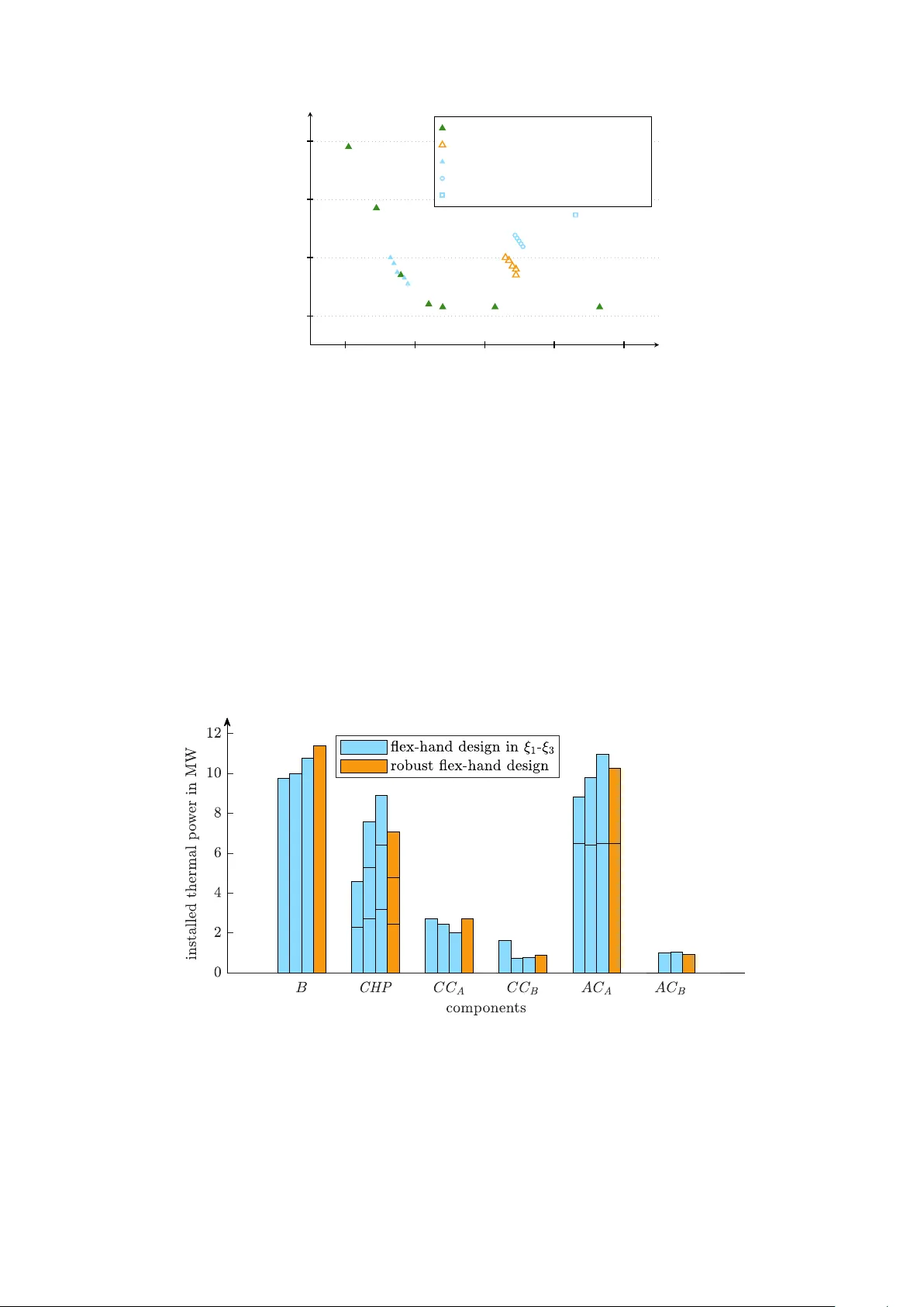
Flexible here-and-no w decisions for t w o-stage m ulti-ob jectiv e optimization: Metho d and application to energy system design selection Dinah Elena Hollermann 1 ∗ , Marc Go erigk 2 † , D ¨ orthe F ranzisca Hoffrogge 1 ‡ , Maik e Hennen 1 § , and Andr ´ e Bardo w 1,3 ¶ 1 Institute of T ec hnical Thermodynamics, R WTH Aac hen Universit y , 52056 Aach en, German y 2 Net w ork and Data Science Managemen t, Universit y of Siegen, 57072 Siegen, Germany 3 Institute of Energy and Climate Researc h, Energy Systems Engineering (IEK-10), F orsc hungszen trum J ¨ ulic h Gm bH, 52425 J ¨ ulic h, German y No v ember 25, 2021 Abstract The syn thesis of energy systems is a t wo-stage optimization problem where design de cisions ha v e to be implemen ted here-and-no w (first s tage), while for the op eration of installed comp onen ts, w e can w ait-and-see (second stage). T o iden tify a sustainable design, w e need to accoun t for b oth economical and environ men tal criteria leading to multi-ob jectiv e optimization problems. Ho w ev er, multi-ob jectiv e optimization leads not to one optimal design but to mu ltiple Pareto- efficien t design options in general. Th us, the decision maker usually has to decide man ually whic h design should finally b e implemen ted. In this pap er, w e prop ose the flexible here-and-no w decision (flex-hand) approach for auto- matic identification of one single design for multi-ob jectiv e optimization. The approach mini- mizes the distance of the Pareto front based on one fixed design to the Pareto fron t allowing m ultiple designs. Uncertaint y regarding parameters of future operations can b e easily include d through a robust extension of the flex-hand approach. Results of a real-w orld case study show that the obtained design is highly flexible to adapt op eration to the considered ob jectiv e functions. Th us, the design pro vides an energy system with the ability to adapt to a changing fo cus in decision criteria, e. g., due to c hanging p olitical aims. Keyw ords Multi-ob jective optimization; automatic solution selection; energy system design; t w o-stage optimization; robust optimization ∗ dinah.hollermann@rwth-aac hen.de † Corrsponding author: marc.go erigk@uni-siegen.de ‡ doerthe.hoffrogge@rwth-aachen.de § maik e.hennen@rwth-aac hen.de ¶ andre.bardo w@ltt.rwth-aac hen.de 1 1 In tro duction The design of sustainable energy systems needs to balance multiple ob jectives represen ting eco- nomical, en vironmen tal, and so cial decision criteria. The resulting design problem is therefore b est addressed b y multi-ob jectiv e optimization. Ho w ever, m ulti-ob jective optimization yields not an optimal design but a P areto fron t with man y differen t designs. Hence, the decision mak er is often confron ted with the question: How to select one single design? In literature, sev eral approaches exist to reduce the n um ber of relev an t solutions, so that the decision maker has then to choose one of few er options. A metho d to fo cus on the relev an t solutions a priori b y excluding solutions b efore the optimization is prop osed by Brank e et al. (2004) and Rachma wati and Sriniv asan (2009). They introduce a preference-based evol utionary approac h fo cusing on calculating “knee” regions of the P areto front. Hennen et al. (2017) fo cus on P areto-efficient solutions whic h are near-optimal with respect to an aggregated criterion that represen ts the o v erall set of ob jective functions. An a p osteriori approac h to reduce the set of relev an t Pareto-efficien t solutions is to cluster solutions, e. g., based on subtractiv e clustering (Zio and Bazzo, 2011), by k -means classification (T ab oada et al., 2007), or by a self-organizing map (Li et al., 2009). Das (1999) fo cus on relev ant P areto-efficien t solutions by ev aluating subsets of the ob jectiv e functions. The approach has b een further developed by Antipov a et al. (2015). But still, in all approaches which reduce the num b er of relev an t solutions, the decision mak er has to select the finally implemented design. F or further reduction of the Pareto-efficien t solutions, T aboada et al. (2007) and Abubak er et al. (2014) prop ose ranking metho ds which are based on a prioritization of ob jectiv e functions b y the decision maker. F or ranking compromising solutions without explicit prioritization, the metho ds LINMAP (Linear Programming T ec hnique for Multidimensional Analysis of Prefer- ence) (Sriniv asan and Sho c ker, 1973), VIKOR (Duckstein and Oprico vic, 1980; Opricovi c and Tzeng, 2004), and TOPSIS (technique for order preference by similarity to an ideal solution) (Hw ang and Y o on, 1981; Chen and Hw ang, 1992) measure the distance from the ideal p oin t and, in TOPSIS, also from the nadir point. The idea is based on compromise programming, where the solution with ob jective v alues “as close as p ossible” t o the ideal p oin t is chosen, or “as far aw ay as p ossible” from the worst p ossible p oin t (Zelan y, 1974). With the aim to determine k ey pla y ers in so cial netw orks, de la F uente et al. (2018) employ eleven metho ds for automatic solution selection within the set of Pareto optimal solutions. These include, e. g., highest hyper- cub e (Beume et al., 2009), consensus (P´ erez et al., 2017), shortest distance to the ideal p oin t (P adh ye and Deb, 2011), and shortest distance to all p oin ts. A review on a p osteriori decision making has b een recentl y prop osed b y Jing et al. (2019). F or general multi-ob jectiv e problems, the int ro duced ranking metho ds are suitable to select one solution. Ho wev er, for synthesi s of energy systems, sp ecial charac teristics of design optimization are b eneficial to select one design. In particular, design optimization of energy systems is a tw o-stage optimization problem. Tw o-stage optimization problems consist of tw o sets of decision v ariables: The her e-and-now variables representing the first stage which need to b e fixed in the b eginning, and the wait-and- se e variables representing the second stage w hic h can still be adapted later (Ben-T al et al., 2004). In energy system optimization, the here-and-now v ariables corresp ond to the design of energy systems while the op eration is determined by the wait-and-see v ariables on the second stage. The approac hes for solution reduction discussed so far do not tak e any adv antage of the t w o-stage c haracteristics of energy systems. Th us, these approaches miss the p ossibilit y to c ho ose a first- stage solution whic h provides high adaptabilit y on the second stage. Exploiti ng adaptabilit y migh t b e particular imp ortan t. Since future conditions are not kno wn to day , the capabilit y to adapt op eration to c hanging circumstances should b e targeted (Shang and Kokossis, 2005). P olitical aims migh t change, and thus, the imp ortance of economical, environmen tal, and so cial 2 aims might c hange. As a result, the sustainable energy system should provide flexible operation to enable an adaptation to a changing fo cus within the regarded criteria. Tw o-stage characterist ics are regarded in design selection b y Mattson and Messac (2003). In the prop osed approac h, the design options need to b e discrete. F or eac h design option, the corresp onding P areto fron t is generated. Afterwards, a P areto filter is applied si m ultaneously to all generated fronts deleting all dominated solutions. Finally , design options lying inside a pre- defined region of in terest are selected. How ever, with increasing num b er of comp onen ts in the giv en sup erstructure, the design options along the Pareto front might change more frequen tly within the region of i n terest leading to a h igher n umber of suitable d esign options to select from. A similar approach is proposed b y Carv alho et al. (2012): Based on discrete design options, the corresp onding Pareto front is generated. Design options with the abilit y to undergo large c hanges in op eration enable higher resilience and are th us fa v ored. Guo et al. (2013) in tro duce a t wo-stage optimal planning and design metho d for combined co oling, heating, and p o wer microgrid systems. On the first stage, the system design is optimized using a generic multi- ob jective optimization approach. On the second stage, the op erational costs are minimized. W ang et al. (2019) additionally regard a feedback from the second stage to the first stage to ensure the accuracy of the planning. Ho w ev er, a systematic or even automatic selection of fa v ored design options is not proposed in either approac hes, e. g., by applying distance measures to assess the generated Pareto fronts. All discussed approac hes do either take adv an tage of the tw o-stage charact eristic of energy systems or prop ose a ranking of Pareto-efficien t solutions. How to select one single design exploiting the t w o-stage nature has not b een prop osed so far to the authors’ b est kno wledge. In this pap er, w e prop ose the flexible her e-and-now de cision (flex-hand) appr o ach to identify one single design which represents the whole P areto front b est without dep ending on an y addi- tional information of the decision maker. F or this purp ose, we minimize the distance b etw een the P areto fron t of the syn thesis problem, i. e., the Pareto fron t with changi ng design options, and the P areto front induced by one fixed design. The fixed design leading to the minimal distance is identified by the prop osed approac h since this design prov ides a high flexibilit y re- garding the considered ob jective functions. Thus, the second stage can b e w ell adapted to a c hanging fo cus from one to another ob jectiv e function. Since not only future aims are uncertain but also future parameter v alues such as demands or costs, w e extend our proposed approach b y considering uncertain input d ata based on scenar- ios. Uncertain ties of input data hav e b een regarded, e. g., b y Quintana et al. (2017); T o ck and Mar ´ ec hal (2015), and Lemos et al. (2018), using the sensitivity against uncertaintie s to assess P areto-efficien t solutions. Gabrielli et al. (2019) prop ose an approach in which P areto-efficien t designs are assessed b y p erformance indicators measuring the robustness and the cost optimal- it y . The final selection of one design dep ends on the target levels which need to b e provided b y the decision maker. Ide and Sch ¨ ob el (2016) provide an ov erview of approac hes for one-stage ro- bust multi-ob jectiv e problems. Robust multi-ob jectiv e optimization has b een applied to energy systems by Ma jewski et al. (2017). Sun et al. (2018) prop ose a multi-ob jectiv e discrete robust optimization algorithm to iden tify a single solution by con v erting multip le ob jectiv e functions in to one unified cost function. Until now, taking uncertain ties in to account when automatically iden tifyingone single design for t w o-stage problems has b een an op en researc h question. F or certain and uncertain tw o-stage problems, our ap proac h allows automatic selection of one design regarding m ultiple decision criteria. While w e introduce our approach in the context of energy systems, the metho dology is general and can b e applied to any t wo-stage m ulti-ob jectiv e optimization problem. The remaining article is structured as follo ws: In Section 2, we introduce the problem class as well as the flex-hand approach and the extension for uncertain input v alues. In the 3 follo wing Section 3, a real-world case study of an industrial park is in troduced and the results are ev aluated. W e give a summary and conclusions in Section 4. 2 The flex-hand approac h for design selection in m ulti-ob jectiv e optimization The selection of energy system designs considering mul tiple criteria is complex, since the Pareto fron t can contain a div erse set of design options. T o help the decision maker implementing one fixed design which allows flexible op eration, we prop ose the flex-hand approach. The approach automatically iden tifies the b est possible design looking even b ey ond the set of P areto solutions. Before present ing the flex-hand approac h in Section 2.2 and the robust extension in Section 2.3, w e first in tro duce some basic concepts and notation in Section 2.1. 2.1 Tw o-stage multi-ob jectiv e optimization Tw o-stage optimization dep ends on t w o stages of decision making. Thus, there are tw o sets of v ariables: X f , the set of feasible solutions for first-stage v ariables x f , and X s ( x f ), the set of feasible solutions for the second-stage v ariables x s whic h dep ends on the chosen first-stage so- lution. First-stage v ariables x f are also called her e-and-now variables since once these v ariables are fixed, they cannot b e adapted later. Second-stage v ariables x s are also called wait-and-se e variables since they can still b e adapted later. As an example, first-stage v ariables x f ma y mo del an inv estment in heating equipment (a design decision), while second-stage v ariables x s mo dels the wa y the equipmen t is run (an op erational decision). In this paper, we use m ultiple ob jectiv es to design sustainabl e energy systems. As ob jectiv es migh t b e conflicting, w e are interested in a set of trade-off solutions. A solution is called Par eto efficient if there is no other solution that is at least as go od in eac h ob jective and strictly b etter in at least one ob jectiv e (Ehrgott, 2005). The tw o-stage m ulti-ob jective problem with K ob jectives is given by: min  f 1 ( x f , x s ) , . . . , f K ( x f , x s )  s.t. x f ∈ X f x s ∈ X s ( x f ) . W e assume the set of Pareto-effici en t solutions to b e discrete and denote them as ( χ f 1 , χ s 1 ) , . . . , ( χ f N , χ s N ). The set of Pareto-efficien t solutions in the ob jective space, called Par eto fr ont , is denoted as P ∗ = ( ρ 1 , . . . , ρ N ) with ρ i = ( ρ i 1 , . . . , ρ i K ) =  f 1 ( χ f i , χ s i ) , . . . , f K ( χ f i , χ s i )  ∈ R K . In this pap er, w e assume that the P areto fron t is discrete; for contin uous Pareto fronts, our approac h is still applicable to a discrete representativ e set of the efficien t solutions. W e call the problem ide al when b oth first-stage v ariables x f and second-stage v ariables x s can b e chosen separately for each efficient p oin t. The corresp onding set of Pareto-efficien t solutions in the ob jective space P ∗ is called ide al Par eto fr ont . The word ide al emphasizes that the ideal P areto front is alwa ys b etter than the Pareto fron t with fixed first-stage v ariables. In energy system optimization, the ideal P areto fron t would imply c hanging design options (e. g. heating equipmen t) along the Pareto fron t and thu s, cannot b e reached b y energy systems implemen ted in the real worl d. In our flex-hand approac h, w e use the ideal Pareto fron t as b enc hmark for ev aluating P areto fronts with fixed design options, i. e., with fixed first-stage v ariables. 4 2.2 The flexible here-and-no w decision approac h The idea of the flex-hand approac h is to find one fixed design which represen ts the ideal Pareto fron t of the synthesis problem b est. In optimization of energy systems, the op er ation of an installed system can b e adapted but chan ging the installed system design is not p ossible in the short term. The design with the highest flexibility in op eration regarding the ob jectiv es is c hosen by the flex-hand approac h. T o determine the highest flexibility , the flex-hand approach minimizes the distance b etw een the ideal Par eto front and the Pareto front based on one fixed design but flexible op eration. The flex-hand approac h is not limited to energy system optimization but can b e applied to an y tw o-stage multi-ob jectiv e problem where the first-stage v ariables x f need to b e fixed righ t no w and the second-stage v ariables x s can b e determined later. F or one fixed design, i. e., for a given first-stage solution x f , w e calculate P areto-efficien t solutions: min  f 1 ( x f , x s ) , . . . , f K ( x f , x s )  s.t. x s ∈ X s ( x f ) . W e obtain a P areto fron t P ( x f ) =  p 1 ( x f ) , . . . , p N ( x f ) ( x f )  dep ending on the first-stage solution x f with N ( x f ) p oin ts whic h w e call fixe d first-stage Par eto fr ont . No w the question arises: Ho w to choose first-stage v ariables x f suc h that we get the “b est” design? T o determine the qualit y of a first-stage solution x f , we compare the Pareto front P ( x f ) with fixed first-stage to the ideal Pareto fron t P ∗ . F or the comparison of t wo sets of m ulti-ob jective solutions, a v ariety of distance measures hav e b een developed (for a review see Zitzler et al. (2003)). Here, we c ho ose a comparison metric based on an additiv e binary ε - indic ator . As discussed by Zitzler et al. (2003), there is no single b est w a y to compare Pareto fron ts, but the ε -indicator is prop osed as a go od o v erall method. Emplo ying other metrics w ould b e p ossible in our setting. F or tw o sets P 1 = ( p 1 , . . . , p S ) and P 2 = ( q 1 , . . . , q T ) in the K -dimensional ob jectiv e space, the binary ε -indicator is obtained by I ( P 1 , P 2 ) = min n ε : ∀ l ∈ [ T ] ∃ j ∈ [ S ] s.t. p j i − q l i ≤ ε ∀ i ∈ [ K ] o where we use the notation [ Z ] = { 1 , . . . , Z } for sets with any integer Z ∈ N . F or our approac h, the measure I  P ( x f ) , P ∗  indicates the distance betw een a fixed first-stage Pareto fron t and the ideal Paret o front . The comparison metric can b e in terpreted as follows: Recall that each point of the ideal P areto front P ∗ ma y inv olve changing first-stage solutions x f along the front. In con trast, the fixed first-stage Pareto front P ( x f ) is based on one single first-stage solution x f where only the second-stage decision can b e adapted. Figure 1 shows the comparison of the ideal P areto fron t to an arbitrary fixed first-stage Pareto front. F or each p oin t on the ideal P areto front, a p oin t on the fixed first-stage P areto fron t can b e determined such that the difference in each ob jective function is smaller than a v alue of ε . By minimizing ε , the distance b et ween the P areto fronts is minimized. In this w a y , for energy systems, w e minimize the distance b etw een the ideal Pare to fron t allo wing c hanging designs as w ell as op eration and the P areto front based on one fixed design where only the op eration can b e adapted. 5 f 1  x f , x s  f 2  x f , x s  ideal Pareto front fixed first-stage Pareto front ≤ ε ≤ ε = ε Figure 1: Comparison of ideal Pareto front to an arbitrary fixed first-stage P areto front, to assess the the quality of the fixed first-stage solutions x f ; dark green dots: ideal Pareto front used as benchmark; orange circles: fixed first-stage Pareto front with distance ε to the ideal P areto fron t; lines are included to guide reader’s eyes Since we consider the difference regarding each ob jectiv e function separately , we normalize the ob jective functions based on the v alue range in P ∗ to circum ven t misleading effects by differen t scales of ob jectiv e v alues. T o this end, we use the normalized ob jectives f i with f i ( x f , x s ) = f i ( x f , x s ) − min j ∈ [ N ] f i ( χ f j , χ s j ) max j ∈ [ N ] f i ( χ f j , χ s j ) − min j ∈ [ N ] f i ( χ f j , χ s j ) . In the following, we write P ( x f ), P ∗ to denote normalized Pareto fronts. Searc hing for an optimal first-stage v ariable x f , i. e., an optimal design, w e now minimize the distance b et ween the P areto fron ts: min n I  P ( x f ) , P ∗  : x f ∈ X f o . The problem formu lation can also b e written as: min ε s.t. f i ( x f , x s j ) − f i ( χ f j , χ s j ) ≤ ε ∀ i ∈ [ K ] , j ∈ [ N ] x f ∈ X f x s j ∈ X s ( x f ) ∀ j ∈ [ N ] . Here, for each p oint on the ideal Pareto front P ∗ , we consider one p oin t on the fixed first-stage P areto front P ( x f ). Thus, for the purp ose of finding an optimal x f , w e assume without loss of generality that the num b er of p oin ts on the fixed first-stage P areto front is identical to the n um b er of p oints on the ideal Pareto front and th us N ( x f ) = N holds. The flex-hand approach yields an optimal first-stage solution ( x f ) ∗ whic h represen ts the ideal Pareto fron t b est regarding the chosen measure. W e call the optimal first-stage solution ( x f ) ∗ the flex-hand solution . In general, the flex-hand solution chosen b y our approach is not necessarily part of the solu tions of the calculated ideal P areto fron t P ∗ . Thus, approac hes based on sorting or solution-reduction would not identify the flex-hand solution in general. Ha ving found a flex-hand solution, w e calculate the corresp onding Pareto-efficien t second- stage solution x s in a separate p ost-pro cessing optimization step. The resulting Pareto fron t is 6 called the flex-hand Par eto fr ont . The n um b er of points on the flex-hand P areto front migh t dif- fer from the original n um b er of points N . F or energy systems, this p ost-pro cessing optimization corresp onds to an op erational multi-ob jectiv e optimization based on a fixed design. There is also an alternative interpretation of our prop osed flex-hand approach: T o solve m ulti-ob jective optimization problems, w eighted sums as P i ∈ [ K ] λ i f i ( x f , x s ) could b e considered (see Ehrgott (2005)). Since w e do not know the correct preference weigh ting, the w eigh ting factors λ i are uncertain. Here, eac h point on the ideal Pareto front represents the optimal solutions if we knew the preference weigh ting in adv ance. The aim is now to find a first-stage solution x f whic h yields a high solution quality for a wide range of weigh ts. The ε v alue of our flex-hand approac h can th us b e considered as regret (see Aissi et al. (2009) for a survey of regret optimization). Ho wev er, employing weigh ted sums, only solutions on the conv ex hull of the P areto front can be found. In con trast, our approach also considers p oin ts not on the con v ex h ull of Pareto solutions. 2.3 The robust flex-hand approac h In optimization of energy systems, decisions are based on input parame ters whic h are inheren tly uncertain. Thus, we extend the prop osed flex-hand approach for problems comprising uncer- tain parameters in the ob jective functions and constraints, and int ro duce the r obust flex-hand appr o ach . As the flex-hand approach, the robust flex-hand approach can also b e applied to an y other tw o-stage m ulti-ob jective problem where the first-stage needs to b e determined in adv ance. The robust flex-hand approach automatically selects first-stage solutions taking uncertain ties in to accoun t. F or this purpose, we assume m ultiple scenarios whic h are con tained in the discrete uncertain ty set U . In each scenario, we compare the ideal P areto fron t for the curren t scenario to a fixed first-stage Par eto front which is based on one fixed set of first-stage v ariables for al l scenarios sim ultaneously . W e then minimize the distance betw een the P areto fron ts in the worst case and thereby find the robust optimal first-stage solution. F or this purpose, we c alculate the ideal P areto front P ∗ ( ξ ) in eac h scenario ξ ∈ U separately . Here, the n umber of el emen ts in P ∗ ( ξ ) is denote d b y N ( ξ ). The ob jectives are parametrized also through scenarios ξ ∈ U , i. e., w e use f i  x f , x s ( ξ ) , ξ  . Again, we normalize ob jectiv es which we denote by f i  x f , x s ( ξ ) , ξ  , for each scenario ξ . T o minimize the worst-case distance b et ween the ideal Pareto front and the fixed first-stage Pareto fron t, we minimize the maximum v alue of the ε -indicator ov er all ξ ∈ U : min ε s.t. f i  x f , x s j ( ξ ) , ξ  − f i  χ f j ( ξ ) , χ s j ( ξ ) , ξ  ≤ ε ∀ ξ ∈ U , i ∈ [ K ] , j ∈ [ N ( ξ )] x f ∈ X f x s j ( ξ ) ∈ X s ( x f , ξ ) ∀ ξ ∈ U , j ∈ [ N ( ξ )] . Here, X s ( x f , ξ ) is the set of feasible second-stage v ariables giv en first-stage v ariables x f and scenario ξ . The optimal first stage solution ( x f ) ∗ is the identi fied robust flex-hand solution. An example is giv en in Figure 2. The ideal Pareto fron t is calculated for each of the three scenarios ( ξ 1 , ξ 2 , ξ 3 ) separately . The robust fixed first-stage Pareto fron ts are based on one fixed set of first-stage v ariables for all scenarios; how ever, the corresp onding robust fixed first-stage P areto fron ts are calculated for each scenario separately by adapting the second-stage v ariables x s . 7 f 1  x f , x s , ξ  f 2  x f , x s , ξ  ideal P areto front in ξ 1 ideal P areto front in ξ 2 ideal P areto front in ξ 3 robust fixed first-stage P areto fron t in ξ 1 robust fixed first-stage P areto fron t in ξ 2 robust fixed first-stage P areto fron t in ξ 3 ≤ ε ≤ ε ≤ ε = ε Figure 2: Idea of the robust flex-hand approac h: F or each scenario separately , the ideal Pareto fron t ( dark green filled marks) and a robust fixed fi rst-stage P areto fron t (orange unfilled marks) are compared; triangles, circles, and squares represent scenario ξ 1 , ξ 2 , and ξ 3 , respectively; the distance ε is calculated regarding all scenarios; here, P areto fronts are presen ted without normalization; lines are included to guide reader’s eyes 3 Case study In this section, w e apply the flex-hand approach to design the energy system of a real-w orld industrial park. The case study is in troduced in Sec tion 3.1. The results of the flex-hand approac h are presen ted and discussed in detail in Section 3.2 and in Section 3.3 for the robust flex-hand approac h. T o compute P areto fron ts, we use the adaptive normal b oundary in tersection metho d (Das and Dennis, 1998). F or calculation, we employ 4 threads of a computer with 3.24 GHz and 64 GB RAM. The problem is form ulated in GAMS 24.7.3 (McCarl and Rosen thal, 2016) and solv ed b y the solv er CPLEX 12.6.3.0 (IBM Corp oration, 2015) to machine accuracy . 3.1 The real-w orld example The real-w orld example is based on our previous work (V oll et al., 2013) on the optimization of a distributed energy supply system. W e consider an industrial site with one p o wer grid, one heating grid and tw o separated co oling grids (Site A and Site B). The thermal demands and their uncertain ties are giv en in Fig. 3. 8 Mar, Apr, Oct May , Sep Jun Jul, Aug Nov – F eb Winter P eak Summer Peak 0 3 6 9 12 thermal energy demands in MW heating demand cooling demand Site A cooling demand Site B Figure 3: Thermal demands of the industrial site and their uncertainti es represented b y error bars; adopted from Ma jewski et al. (2017) The design of the energy system corresp onds to sizing and installing any n um b er of com- p onen ts from the follo wing types of energy conv ersion comp onent s: b oilers B , combined heat and p ow er engines CHP , absorption c hillers AC , and compression c hillers C C . Natural gas can b e used at costs of p g as = 6 ct / kWh with ± 40 % of uncertain t y . F urthermore, w e assume a connection to the electricity grid. Electricit y can b e purchased for p el,buy = 16 ct / kWh and sold for p el,sell = 10 ct / kWh. F or purchasing and selling, an uncertaint y of ± 46 % is considered. All p ossibly uncertain input parameters dep end on the scenario ξ and are additionally marked using a tilde. The v alues for uncertaint y are deduced from Ma jewski et al. (2017). T o design a sustainable energy system, we emplo y an economical and an environmen tal ob jectiv e function: the total annualized costs T AC and the global warming impact GWI . In principle, the metho d could also consider so cial criteria (Mota et al., 2015). The total annual ized costs T AC are defined by: T AC  ˙ U , ˙ U el,buy , ˙ V el,sell , INVEST k ; ξ  (1) = X t ∈ [ T ] h ∆ τ t  e p g as ( ξ ) · X k ∈ B ∪ CHP ˙ U kt ( ξ ) + e p el,buy ( ξ ) · ˙ U el,buy t ( ξ ) − e p el,sell ( ξ ) · ˙ V el,sell t ( ξ ) i + X k ∈K  1 PVF + p m k  · INVEST k Here, k represents a comp onen t in the set of all comp onents K = B ∪ CHP ∪ AC ∪ C C which migh t b e installed. F or each time step t ∈ [ T ], ∆ τ t represen ts its length. The corresp onding input energy flows of natural gas for b oilers B and combined heat and p o wer engines CHP are denoted by ˙ U kt . The input and the output energy flow of electricity are declared by ˙ U el,buy t and ˙ V el,sell t , resp ectiv ely . F or each comp onen t k , p m k represen ts the annual maintenance costs as share of the in v estmen t costs INVEST k . F or ann ualizing the inv estment costs INVEST k , we use the present v alue factor (Brov erman, 2010) PVF = ( i + 1) h − 1 ( i + 1) h · i with an inter est rate i = 8 % and a time horizon h = 4 a. 9 The global warming impact is given by: GWI  ˙ U , ˙ U el,buy , ˙ V el,sell ; ξ  (2) = X t ∈ [ T ] ∆ τ t " X k ∈ B ∪ CHP ˙ U kt ( ξ ) · GWI g as +  ˙ U el,buy t ( ξ ) − ˙ V el,sell t ( ξ )  · ] GWI el ( ξ ) # . W e emplo y GWI g as = 244 g CO 2 -eq. / kWh for the sp ecific global warmin g impact of gas whic h is not sub ject to remark able v ariation. F or the specific global w arming impact GWI el of electricit y purc hased from the grid, w e employ a v alue of 561 g CO 2 -eq. / kWh. Since the future electricit y mix migh t c hange significan tly , w e assume the sp ecific global w arming impact GWI el to b e uncertain lying within 430 g CO 2 -eq. / kWh and 610 g CO 2 -eq. / kWh. When selling electricit y to the grid, a credit for global warming impact is given, following the idea of the a v oided burden (Baumann and Tillman, 2004). Here, the global warmin g impact GWI dep ends only implicitly on the first-stage v ariables x f due to the constraints. A direct influence would b e giv en if the global warming impact induced b y the manufactur ing of the comp onents was tak en in to accoun t. Ho wev er, since the global warming impact of the op eration has usually a significan tly higher impact (Guill ´ en-Gos´ alb ez, 2011), we neglect this dependency . The complete flex-hand optimization mo del is presented in App endix A. F or the design optimization, we assume a “green field” without existing energy comp onen ts. Ho w ev er, the flex-hand approac h could also b e applied to retrofit an energy system. 3.2 The flex-hand design W e no w employ the flex-hand approach to design the sustainable energy system in order to obtain the b est solution for the first-stage v ariables x f whic h we call the flex-hand design . F or this purp ose, we first calculate the ideal Par eto front as a b enc hmark. The ideal Pareto front is obtained by allowing a different design for eac h p oin t on the front. The largest optimization problem for calculating a point on the ideal P areto fron t consists of 1950 equations, 576 v ariables, and 310 binary v ariables after presolve. In total, the whole ideal P areto front is calculated in 317 s. The flex-hand problem has 5099 equations, 2023 v ariables, and 751 binary v ariables after presolv e. Here, computing the flex-hand P areto front takes 152 s. Both the ideal Pareto front and the flex-hand Pareto front are shown in Fig. 4. 10 7 . 5 8 8 . 5 9 9 . 5 22 23 24 25 26 T A C in Mio. e /a GWI in kt CO 2 -eq. / a ideal Pareto fron t flex-hand Pareto fron t fixed first-stage Pareto fronts of ideal designs = ε ∗ Figure 4: Comparison of ideal P areto front (dark green dots) and the flex-hand P areto fron t (orange circles) with minimal distance ε ∗ to the ideal P areto fron t; small dark green dots: fixed first-stage P areto front of ideal designs, i. e., Pareto-efficien t op eration for eac h design of the ideal Pareto fron t; here, Pare to fronts are presented without normalization; lines are included to guide reader’s eyes The flex-hand P areto fron t of the selected design is “strec hed out” . Thus, the flex-hand design allo ws for flexible op eration pro viding a high ability to adapt to c hanging future ob jectives . The flex-hand design can b e op erated such that the total annualized costs T AC are v ery low at 7 . 8 Mio. e / a or the global warming impact GWI is very low with 22 . 6 kt CO 2 -eq. / a. In this case study , the minimal distance betw een the ideal and the flex-hand Pareto fron t is limited, e. g., by the anchor p oin ts with minimal total annualized costs limits (Fig. 4). The corresp onding scaled v alue for the minimized distance is ε ∗ = 0 . 128. F or unscaled v alues, the minimal total ann ualized costs for the ideal design are T A C ideal = 7 . 51 Mio. e / a and for the flex- hand design T A C f l ex - hand = 7 . 78 Mio. e / a, resp ectively . Hence, the maximal deviation for total ann ualized costs is 0 . 27 Mio. e / a whic h corresponds to a maximal loss of only 3 . 6 % compared to the ideal design with minimized total annualized costs. Regarding the minimal global w arming impact, the maximal deviation is only 2 . 17 %. Thus, the flexibilit y of the flex-hand design is v ery high regarding b oth ob jective functions. When ha ving a closer lo ok at the iden tified design, w e cannot iden tify a single reason for its higher abilit y to adapt op eration (Fig. 5). 11 Figure 5: In dark green: designs of ideal Pareto front; in orange: flex-hand design of the flex- hand Pareto front; from left to right, the designs are ordered by decreasing minimal global w arming impact; B b oiler, CHP combined heat and p o w er engine, C C A and C C B compression c hillers, and AC A and AC B absorption c hillers installed on Site A and Site B, resp ectivel y In general, solutions with low er global warming impact prefer installing higher capacit y of com bined heat and pow er engines, since the specific global w arming impact of the electricit y mix of the grid is higher than the impact of the combined heat and p o wer engines in combination with absorption chillers. The flex-hand design do es not sho w remark able differences compared to the other ideal designs but pro vides an excellent compromise. Without the prop osed approac h, this highly adaptable design would most likely not hav e b een identified by the decision maker. 3.3 The robust flex-hand design W e now apply the robust flex-hand approac h to the prop osed case study taking uncertainties in to account. The uncertain ties are introduced in Section 3.1. Here, we consider three scenarios ξ 1 , ξ 2 , and ξ 3 . Scenario ξ 2 corresp onds to v alues of the problem without uncertainties discussed in Section 3.2. In scenario ξ 1 , we assume all uncertain v alues to tak e their smallest v alues wit hin the uncertain t y range and in scenario ξ 3 their largest v alues, resp ectiv ely . Ho w ev er, any other scenario could b e c hosen. 12 4 6 8 10 12 14 20 25 30 35 ξ 1 ξ 2 ξ 3 T A C in Mio. e /a GWI in kt CO 2 -eq. / a Figure 6: T riangles, circles, and squares represen t scenario ξ 1 , ξ 2 , and ξ 3 , resp ectiv ely; dark green filled marks: ideal Pareto fron t generated for eac h scenario separately , orange unfilled marks: robust flex-hand Pareto fron t in each scenario; small light blue marks: flex-hand P areto front for separately considered scenarios; here, Paret o fronts are presented without normalization T o ev aluate the robust flex-hand design, we compare the robust flex-hand Pareto fronts in all three scenarios to the flex-hand Pareto fron ts generated for each scenario separately . Fig. 6 sho ws that the flex-hand Pareto fronts generated for each scenario separately do not coincide with the robust flex-hand Pareto fron ts. In scenario ξ 3 , the robust flex-hand design leads to smaller total ann ualized costs than the flex-hand design computed for scenario ξ 3 but to a higher global warming impact. In total, the robust flex-hand Par eto fron t is less “streched out” than for the nominal case (Section 3.2) leading to an optimal distance ε ∗ of 0 . 625. The reduced adaptability to the ideal Pareto fron ts is due to the fact that the robust flex-hand P areto fron ts need to appro ximate three ideal Pareto fronts simultaneously , instead of just one P areto front. Thus, a go o d p erformance of a flex-hand design in one scenario might lead to a p oor p erformance in another scenario if uncertainties are not regarded during design (Fig. 7). In cont rast, the robust flex-hand design is a compromise solution p erforming well in all three scenarios sim ultaneously . In Fig. 7, w e take a closer lo ok on the computed Par eto fronts in scenario ξ 1 . Here, the robust flex-hand design ( 4 ) clearly p erforms b etter than the flex-hand design identified for scenario ξ 2 ( ◦ ) and the flex-hand design identified for scenario ξ 3 (    ). In scenario ξ 1 , only the flex-hand P areto fron t of scenario ξ 1 ( N N N ) appro ximates the ideal Par eto fron t ( N N N ) b etter than the robust flex-hand Pareto fron t ( 4 ). Ho w ev er, the flex-hand design of scenario ξ 1 is infeasible for scenario ξ 2 and ξ 3 . In contrast, the robust flex-hand design is feasible and p erforms w ell for all scenarios. 13 3 . 6 3 . 8 4 4 . 2 4 . 4 17 . 4 17 . 6 17 . 8 18 T A C in Mio. e /a GWI in kt CO 2 -eq. / a ideal Pareto fron t of ξ 1 robust flex-hand Pareto fron t in ξ 1 flex-hand Pareto fron t of ξ 1 flex-hand Pareto fron t of ξ 2 in ξ 1 flex-hand Pareto fron t of ξ 3 in ξ 1 Figure 7: All Pareto fronts for scenario ξ 1 ; dark green filled triangles ( N N N ): ideal Pareto front of scenario ξ 1 ; orange unfilled triangles ( 4 ): robust flex-hand Pareto front in scenario ξ 1 ; small ligh t blue triangles ( N N N ): flex-hand P areto fron t of scenario ξ 1 ; small ligh t blue unfill ed circles and squares ( ◦ and    ): flex-hand Pareto front in scenario ξ 1 based on flex-hand design computed for scenario ξ 2 and ξ 3 , resp ectiv ely; here, Pareto fronts are presen ted without normalization Ha ving a closer lo ok at the design (Fig. 8), we observe that the total capacity of the three flex-hand designs increases from scenario ξ 1 to ξ 3 . This is due to the fact that v alues of uncertain input parameter increase as well. With increasing demands and also increasing sp ecific global w arming impact of the electricit y grid, larger combined heat and p o wer engines and b oilers are installed com bined with a higher capacit y of absorption chillers and smaller compression chillers. The robust flex-hand design do es not differ remark ably from the three flex-hand designs. Thus, the robust flex-hand approac h is necessary to iden tify the excellen t compromise given by the robust flex-hand design. Figure 8: In ligh t blue: flex-hand designs generated for each scenario separately (from left to righ t: scenario ξ 1 , ξ 2 , and ξ 3 ); in orange: robust flex-hand design; B b oiler, CHP com bined heat and p ow er engine, C C A and C C B compression chillers, and AC A and AC B absorption chillers installed on Site A and Site B, resp ectivel y 14 4 Conclusions The sustainable optimization of energy systems is inheren tly a tw o-stage optimization prob- lem with m ultiple decision criteria. Applying m ulti-ob jective optimization usually generates differen t designs for eac h p oin t on the P areto fron t. W e propose the flex-hand approac h for iden tifying a single design which p erforms w ell regarding all decision criteria. The idea of the flex-hand approach is to approximate the P areto fron t with changing design options ( ide al Par eto fr ont ) by a Pareto front with one fixed design for the whole front. The design leading to the minimal distance b et ween b oth Pareto fron ts is the design which is iden tified by the flex-hand approac h. The iden tified design ( flex-hand design ) is able to adapt to all regarded criteria w ell, and thus, provides high flexibilit y to reach future aims for which fo cus might c hange b et w een the considered ob jective functions. Our real-world case study demonstrates the resulting high adaptability with resp ect to the considered criteria. F or designing the sustainable energy system, we c ho ose total annualized costs and the global w arming impact as economical and environmen tal criteria, resp ectiv ely . The calculated Paret o front of the flex-hand design is ” stretc hed out” in comparison to the P areto fronts obtained by op erational optimization of designs lying on the ideal Pareto front. The ob jectiv e function v alues of flex-hand design differ by less than 3 . 6 % from the ideal v alues whic h highlights the excellen t quality of the iden tified flex-hand design. The flex-hand design do es not show remark able differences compared to the designs lying on the ideal Pareto front. Th us, without the flex-hand approac h, the decision maker would p ossibly not ha ve chosen the iden tified design. This effect b ecomes ev en more pronounced when considering mul tiple scenarios simultaneously to account for uncertaint y , in which case our approach is able to find a robust solution. T o conclude, the flex-hand approac h tak es adv antage of the tw o-stage nature of energy systems to automatically select one single design whic h pro vides a high flexibility to adapt op eration to all considered criteria. Ac kno wledgmen ts This w ork w as supported b y the Helmholtz Association under the Joint Initiative Energy System 2050—A Cont ribution of the Research Field Energy . A Mo del F orm ulation In the following, we pro vide the problem formul ation of the robust flex-hand optimization for the DESS considered in our case study (Section 3). In the case study , we consider the total ann ualized costs T A C and the global warming impact GWI as ob jective functions. Uncertainties are regarded for tariffs for purchasing gas e p g as ( ξ ) and electricity e p el,buy ( ξ ) as well as for selling electricit y e p el,sell ( ξ ). F urthermore, the sp ecific global warming impact of the electricit y mix of the grid ] GWI el ( ξ ) is assumed to b e uncertain as w ell. In the constraints, the energy balances are affected by uncertain energy demands e ˙ E heat ( ξ ) , e ˙ E cool ( ξ ), and e ˙ E el ( ξ ). 15 min ε s.t. T AC  ˙ U , ˙ U el,buy , ˙ V el,sell , γ , ˙ V N ; ξ , j  − T A C ∗ ( ξ , j ) ≤ ε ∀ ξ ∈ U , j ∈ [ N ( ξ )] GWI  ˙ U , ˙ U el,buy , ˙ V el,sell ; ξ , j  − GWI ∗ ( ξ , j ) ≤ ε ∀ ξ ∈ U , j ∈ [ N ( ξ )] X k ∈ B ∪ CHP ˙ V kt ( ξ , j ) − X k ∈ AC ˙ U kt ( ξ , j ) = e ˙ E heat t ( ξ ) ∀ t ∈ [ T ] , ξ ∈ U , j ∈ [ N ( ξ )] X k ∈ AC ∪ C C ˙ V kt ( ξ , j ) = e ˙ E cool t ( ξ ) ∀ t ∈ [ T ] , ξ ∈ U , j ∈ [ N ( ξ )] X k ∈ CHP ˙ V el kt ( ξ , j ) − X k ∈ C C ˙ U kt ( ξ , j ) + ˙ U el,buy t ( ξ , j ) − ˙ V el,sell t ( ξ , j ) = e ˙ E el t ( ξ ) ∀ t ∈ [ T ] , ξ ∈ U , j ∈ [ N ( ξ )] X h ∈ [ H ] γ kh ≤ 1 ∀ k ∈ K γ kh · ˙ V N ,lb kh ≤ ˙ V N kh ≤ γ kh · ˙ V N ,lb kh +1 ∀ k ∈ K , ∀ h ∈ [ H ] ρ min · X h ∈ [ H ] ˙ V N kh ≤ ˙ V kt ( ξ , j ) ≤ X h ∈ [ H ] ˙ V N kh ∀ k ∈ K , t ∈ [ T ] , ξ ∈ U , j ∈ [ N ( ξ )] ˙ V kt ( ξ , j ) = η k · ˙ U kt ( ξ , j ) ∀ k ∈ K , t ∈ [ T ] , ξ ∈ U , j ∈ [ N ( ξ )] ˙ V el kt ( ξ , j ) = η tot k · ˙ U kt ( ξ , j ) − ˙ V kt ( ξ , j ) ∀ k ∈ CHP , t ∈ [ T ] , ξ ∈ U , j ∈ [ N ( ξ )] ε ∈ R + ˙ U el,buy ( ξ , j ) , ˙ V el,sell ( ξ , j ) , ˙ V el ( ξ , j ) , ˙ U ( ξ , j ) , ˙ V ( ξ , j ) ∈ R |K|× T + ∀ ξ ∈ U , j ∈ [ N ( ξ )] γ ∈ { 0 , 1 } |K|× H , ˙ V N ∈ R |K|× H + The total annuali zed costs T AC and the global warming impact GWI are defined b y T AC  ˙ U , ˙ U el,buy , ˙ V el,sell , γ , ˙ V N ; ξ , j  = X t ∈ [ T ] h ∆ τ t  e p g as ( ξ ) · X k ∈ B ∪ CHP ˙ U kt ( ξ , j ) + e p el,buy ( ξ ) · ˙ U el,buy t ( ξ , j ) − e p el,sell ( ξ ) · ˙ V el,sell t ( ξ , j ) i + X k ∈K  1 PVF + p m k  · X h ∈ [ H ] h γ kh · κ kh + m kh ·  ˙ V N kh − γ kh ˙ V N ,lb kh i | {z } = : INVEST k GWI  ˙ U , ˙ U el,buy , ˙ V el,sell ; ξ , j  = X t ∈ [ T ] ∆ τ t " X k ∈ B ∪ CHP ˙ U kt ( ξ , j ) · GWI g as +  ˙ U el,buy t ( ξ , j ) − ˙ V el,sell t ( ξ , j )  · ] GWI el ( ξ ) # . Bars ab o v e the total annualized costs T A C and the global warming impact GWI in the opti- mization problem denote the normalization of the ob jective v alues. Ob jectiv e v alues on the nor- malized ideal Pareto fronts are denoted by  T AC ∗ ( ξ , j ) , GWI ∗ ( ξ , j )  for each p oin t j ∈ [ N ( ξ )] and eac h scenario ξ in the uncertaint y set U . 16 The duration of a time step t ∈ [ T ] is given by ∆ τ t . Maintenance costs are determined b y the share p m k of the in v estmen t costs INVEST k . The inv estment costs INVEST k are ann ual- ized by the presen t v alue factor PVF . GWI g as represen t the specific global w arming impact of purc hased gas. Purchased and sold electricit y is denoted by ˙ U el,buy t and ˙ V el,sell t , resp ectiv ely . ˙ U kt and ˙ V kt sp ecifies input and output energy flows in time step t of comp onen t k ∈ K . Com- p onen ts include b oilers B , combined heat and p o wer engines CHP , absorption c hillers AC , and compression chillers C C . Input and output energy flo ws are coupled b y the thermal efficiency η k . F or combined heat and pow er engines, the total efficiency η tot k is giv en by the sum of the thermal and the electrical efficiency η tot k = η k + η el k . The minimal part-load of a comp onen t k is defined b y the fraction ρ min of the installed nominal capacity . The in vestmen t costs INVEST k of a newly installed component k are linearized b y piecewise linearization with P h ∈ [ H ] h γ kh · κ kh + m kh ·  ˙ V N kh − γ kh ˙ V N ,lb kh i (see Fig. 9). m kh is the gradien t for eac h line segment h ∈ [ H ] and is defined by m kh : = κ kh +1 − κ kh ˙ V N ,lb kh +1 − ˙ V N ,lb kh ∀ k ∈ K , h ∈ [ H ] . Here, parameters ˙ V N ,lb kh +1 and ˙ V N ,lb kh represen t the nominal capacities of the low er and upp er supp orting p oin t of line segment h and parameters κ kh and κ kh +1 the corresponding sp ecific in v estment costs. Binary v ariables γ kh determine if line segmen t h is active ( γ kh = 1). Since the sum P h ∈ [ H ] γ kh is equal to 1, only one line segment can b e activ e at the time. Th us, only one v alue for the nominal capacit y ˙ V N kh of all line segments is unequal to 0; hence, the nominal capacit y ˙ V N k of an installed comp onen t k is given by the sum P h ∈ [ H ] ˙ V N kh . ˙ V N k INVEST k ˙ V N k ˙ V N,lb kh − 1 κ kh − 1 ˙ V N,lb kh κ kh ˙ V N,lb kh +1 κ kh +1 ˙ V N kh h − 1 h m kh − 1 m kh Figure 9: Piecewise linearization of the in v estment costs INVEST k of a newly installed comp o- nen t k is presented. Here, h is the active line segment; thus, γ kh is equal to 1. References Abubak er, A., Baharum, A., and Alrefaei, M. (2014). Go o d solution for multi-ob jectiv e opti- mization problem. AIP Conf. Pr o c. , 1605(1):1147–1152. Aissi, H., Bazgan, C., and V anderp o oten, D. (2009). Min–max and min–max regret ver sions of com binatorial optimization problems: A surv ey . Eur. J. Op er. R es. , 197(2):427–438. 17 An tipov a, E., P ozo, C., Guill ´ en-Gos´ alb ez, G., Bo er, D., Cab eza, L., and Jim´ enez, L. (2015). On the use of filters to facilitate the p ost-optimal analysis of the Pareto solutions in multi- ob jective optimization. Comput. Chem. Eng. , 74:48–58. Baumann, H. and Tillman, A.-M. (2004). The Hitch Hiker’s Guide to LCA . Stu den tlitteratur AB. Ben-T al, A., Gory ashk o, A., Guslitzer, E., and Nemirovski, A. (2004). Adjustable robust solu- tions of uncertain linear programs. Math Pr o gr am , 99(2):351–376. Beume, N., F onseca, C. M., Lop ez-Ibanez, M., Paque te, L., and V ahrenhold, J. (2009). On the complexit y of computing the hyperv olume indicator. IEEE T. Evolut. Comput. , 13(5):1075– 1082. Brank e, J., Deb, K., Dierolf, H., and Ossw ald, M. (2004). Finding knees in multi-ob jectiv e optimization. In Y ao, X., Burke, E. K., Lozano, J. A., Smit h, J., Merelo-Guerv´ os, J. J., Bullinaria, J. A., Row e, J. E., Ti ˇ no, P ., Kab´ an, A., and Sc hw efel, H.-P ., editors, Par al lel Pr oblem Solving fr om Natur e - PPSN VIII , pages 722–731, Berlin, Heidel b erg. Springer Berlin Heidelb erg. Bro v erman, S. A. (2010). Mathematics of Investment and Cr e dit . ACTEX Publications, Inc., 5th edition. Carv alho, M., Lozano, M. A., and Serra, L. M. (2012). Multicriteria syn thesis of trigeneration systems considering economic and envir onmen tal asp ects. Appl. Ener gy , 91(1):245–254. Chen, S.-J. and Hw ang, C.-L. (1992). F uzzy Multiple Attribute De cision Making Metho ds , pages 289–486. Springer Berlin Heidelb erg, Berlin, Heidelb erg. Das, I. (1999). A preference ordering among v arious Pareto optimal alternatives. Struct. Opti- mization , 18(1):30–35. Das, I. and Dennis, J. E. (1998). Normal-b oundary intersection: A new metho d for generat- ing the Pareto surface in nonlinear mult icriteria optimization problems. Siam. J. Optim. , 8(3):631–657. de la F uente, D., V ega-Ro dr ´ ıguez, M. A., and P ´ erez, C. J. (2018). Automatic selection of a single solution from the Pareto front to identify k ey play ers in so cial net w orks. Know l.-Base d Syst. , 160:228–236. Duc kstein, L. and Oprico vic, S. (1980). Multiob jective optimization in river basin dev elopment. Water. R esour. R es. , 16(1):14–20. Ehrgott, M. (2005). Multicriteria Optimization . Springer Berlin Heidelb erg, 2 edition. Gabrielli, P ., F ¨ urer, F., Mavromatidis, G., and Mazzotti, M. (2019). Robust and optimal design of m ulti-energy systems with seasonal storage through uncertaint y analysis. Appl. Ener gy , 238:1192–1210. Guill ´ en-Gos´ alb ez, G. (2011). A no v el MILP-based ob jective reduction metho d for multi- ob jective optimization: Application to environmen tal problems. Comput. Chem. Eng. , 35(8):1469–1477. 18 Guo, L., Liu, W., Cai, J., Hong, B., and W ang, C. (2013). A tw o-stage optimal planning and design metho d for combined co oling, heat and p o wer microgrid system. Ener gy Conversion and Management , 74:433–445. Hennen, M., Postels, S., V oll, P ., Lamp e, M., and Bardow, A. (2017). Multi-ob jective synthesis of energy systems: Efficien t identificati on of design trade-offs. Comput. Chem. Eng. , 97:283– 293. Hw ang, C.-L. and Y o on, K. (1981). Metho ds for Multiple Attrib ute De cision Making , pages 58–191. Springer Berlin Heidelb erg, Berlin, Heidelb erg. IBM Corp oration (2015). IBM ILOG CPLEX Optimization Studio, V ersion 12.6. User Guide. Ide, J. and Sch ¨ ob el, A. (2016). Robustness for uncertain multi-ob jectiv e optimization: a survey and analysis of different concepts. OR Sp e ctrum , 38(1):235–271. Jing, R., W ang, M., Zhang, Z., Liu, J., Liang, H., Meng, C., Shah, N., Li, N., and Zhao, Y. (2019). Comparativ e study of p osteriori decision-making methods when designing building in tegrated energy systems with m ulti-ob jectives. Ener gy and Buildings , 194:123 – 139. Lemos, L. P ., Lima, E. L., and Pinto, J. C. (2018). New decision making criterion for multiob- jectiv e optimization problems. Ind. Eng. Chem. R es. , 57(3):1014–1025. Li, Z., Liao, H., and Coit, D. W. (2009). A t wo-stage appr oac h for m ulti-ob jective decision mak- ing with applications to system reliabilit y optimization. R eliab. Eng. Syst. Safe. , 94(10):1585– 1592. Ma jewski, D. E., Wirtz, M., Lamp e, M., and Bardo w, A. (2017). Robust multi-ob jectiv e optimization for sustainable design of distributed energy supply systems. Comput. Chem. Eng. , 102:26–39. Mattson, C. A. and Messac, A. (2003). Concept selection using s-Pareto frontiers. AIAA J. , 41(6). McCarl, B. A. and Rosenthal, R. E. (2016). McCarl GAMS User Guide, V ersion 24.7. Mota, B., Gomes, M. I., Carv alho, A., and Barb osa-P o v oa, A. P . (2015). T o wards supply c hain sustainabilit y: economic, environmen tal and so cial design and planning. J. Cle an. Pr o d. , 105:14–27. Oprico vic, S. and Tzeng, G.-H. (2004). Compromise solution by MCDM metho ds: A compara- tiv e analysis of VIKOR and TOPSIS. Eur. J. Op er. R es. , 156(2):445 – 455. P adh ye, N. and Deb, K. (2011). Multi-obje ctive Optimisation and Multi-criteria De cision Mak- ing for FDM Using Evolutionary Appr o aches , pages 219–247. Springer London, London. P ´ erez, C. J., V ega-Rodr ´ ıguez, M. A., Reder, K., and Fl ¨ ork e, M. (2017). A multi-ob jectiv e artificial b ee colon y-based optimization approac h to design w ater qual it y monitoring net w orks in riv er basins. J. Cle an. Pr o d. , 166:579–589. Quin tana, D., Den ysiuk, R., Garcia-Ro driguez, S., and Gaspar-Cunha, A. (2017). Portfolio implemen tation risk management using evolutionary m ultiob jective optimization. Appl. Sci. , 7(10):1079. 19 Rac hma w ati, L. and Sriniv asan, D. (2009). Multiob jectiv e evolutionary algorithm with control- lable fo cus on the knees of the Pareto front. IEEE T. Evolut. Comput. , 13(4):810–824. Shang, Z. and Kok ossis, A. (2005). A systematic approac h to the syn thesis and design of flexible site utilit y systems. Chem. Eng. Sci. , 60(16):4431–4451. Sriniv asan, V. and Sho c ker, A. D. (1973). Linear programming techniques for multidimensional analysis of preferences. Psychometrika , 38(3):337–369. Sun, G., Zhang, H., F ang, J., Li, G., and Li, Q. (2018). A new multi-ob jectiv e discrete robust optimization algorithm for engineering design. Appl. Math. Mo del. , 53:602–621. T ab oada, H. A., Baheranw ala, F., Coit, D. W., and W attanap ongsak orn, N. (2007). Prac- tical solutions for multi-ob jectiv e optimization: An application to system reliabilit y design problems. R eliab. Eng. Syst. Safe. , 92(3):314 – 322. T o c k, L. and Mar ´ echal , F. (2015). Decision supp ort for ranking Pareto optimal pro cess designs under uncertain mark et conditions. Comput. Chem. Eng. , 83:165–175. V oll, P ., Klaffk e, C., Hennen, M., and Bardow, A. (2013). Automated sup erstructure-based syn thesis and optimization of distributed energy supply systems. Ener gy , 50:374–388. W ang, Y., W ang, Y., Huang, Y., Li, F., Zeng, M., Li, J., W ang, X., and Zhang, F. (2019). Planning and operation method of th e regional in tegrated energy system cons idering econom y and en vironmen t. Ener gy , 171:731–750. Zelan y , M. (1974). A concept of compromise solutions and the metho d of the displaced ideal. Comput. Op er. R es. , 1(3-4):479–496. Zio, E. and Bazzo, R. (2011). A clustering pro cedure for reducing the n um ber of represen tativ e solutions in the Pareto fron t of multiob jectiv e optimization problems. Eur. J. Op er. R es. , 210(3):624–634. Zitzler, E., Thiele, L., Laumanns, M., F onseca, C. M., and da F onseca, V. G. (2003). Per- formance assessment of multiob jectiv e optimizers: an analysis and review. IEEE T. Evolut. Comput. , 7(2):117–132. 20