Engineering and Business Applications of Sum of Squares Polynomials

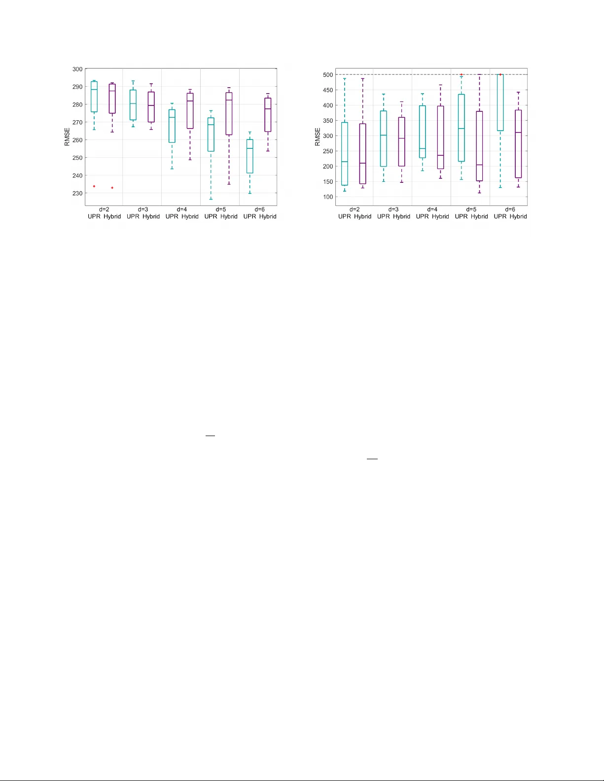
Proceedings of Symposia in Applied Mathematics Engineering and Business Applications of Sum of Squares P olynomials Georgina Hall Abstract. Optimizing over the cone of nonnegative p olynomials, and its dual counterpart, optimizing ov er the space of moments that admit a representing measure, are fundamental problems that app ear in man y diﬀerent applications from engineering and computational mathematics to business. In this paper, we review a number of these applications. These include, but are not limited to, problems in control (e.g., formal safety veriﬁcation), ﬁnance (e.g., option pricing), statistics and mac hine learning (e.g., shape-constrained regression and optimal design), and game theory (e.g., Nash equilibria computation in polynomial games). W e then show how sum of squares techniques can be used to tackle these problems, which are hard to solve in general. W e conclude by highlighting some directions that could be pursued to further disseminate sum of squares techniques within more applied ﬁelds. Among other things, we brieﬂy address the current challenge that scalability represents for optimization problems that inv olv e sum of squares p olynomials and discuss recent trends in softw are developmen t. A v ariet y of applications in engineering, computational mathematics, and business can b e cast as optimization problems o v er the cone of nonnegativ e polynomials or the cone of moments admitting a represen ting measure. F or a long while, these problems were though t to b e intractable until the adven t, in the 2000s, of tec hniques based on sum of squares (sos) optimization. The goal of this pap er is to provide concrete examples—from a wide v ariety of ﬁelds—of settings where these techniques can b e used and detailed explanations as to ho w to use them. The pap er is divided in to four parts, eac h corresp onding to a broad area of in terest: P art 1 co v ers control and dynamical systems, Part 2 co vers probability and measure theory , P art 3 cov ers statistics and mac hine learning, and P art 4 cov ers optimization and game theory . Eac h part is further sub divided into sections, which corresp ond to sp eciﬁc problems within the broader area such as, for Part 1, certifying prop erties of a p olynomial dynamical system. Eac h section is purp osefully written so that limited knowledge of the application ﬁeld is needed. Consequen tly , a large part of eac h section is sp en t on providing a mathematical framework for the ﬁeld and couching the question of interest as an optimization problem inv olving nonnegative p olynomials and/or moment constraints. A shorter part explains how to go from these (in tractable) problems to (computationally-tractable) sos programs. The conclusion of this pap er brieﬂy touches up on some implementation challenges faced b y sum of squares optimization and the subsequen t research eﬀort developed to coun ter them. P art 1. Dynamical systems and control A dynamical system is a system whose state v aries ov er time. Broadly sp eaking, a state is a v ector x ( t ) ∈ R n that pro vides enough information on the system at time t for one to predict future v alues of the state if the system is left to its o wn devices. F or example, if w e consider a physical system suc h as a rolling ball, then one could, e.g., consider the position and instantaneous velocity of its cen ter as a 6-dimensional state vector. Or, if the problem at hand is a study of the evolution of the p opulation of wolv es and sheep in a certain geographical region, the state vector of a simple mo del could simply encompass the curren t num ber of w olves and sheep in that region. As the state vector con tains enough information that one can predict its ev olution if there is no outside interference, it is p ossible to relate future states bac k to the current state via so-called state e quations . Their expression v aries dep ending on whether the system is discr ete time or c ontinuous time . In a discrete-time system, the state x ( k ) is deﬁned for discrete times k = 0 , 1 , 2 , . . . , and w e hav e x ( k + 1) = f ( x ( k )) , (0.1) 2000 Mathematics Subject Classiﬁc ation. 49-06,49-02,90C22,90C90. Key wor ds and phr ases. Sum of squares optimization, engineering applications, dynamical systems and con trol, momen t problems, option pricing, shap e-constrained regression, optimal design, p olynomial games, cop ositiv e and robust semideﬁnite optimization. c  0000 (copyright holder) 1 2 GEORGINA HALL where f is some function from R n to R n . In a con tinuous-time system, the state x ( t ) v aries contin uously with time t ≥ 0 and w e hav e dx ( t ) dt = f ( x ( t )) , (0.2) where f is again some function from R n to R n . The goal is generally to understand how the tr aje ctory { x ( k ) } k , solution to (0.1), or t 7→ x ( t ), solution to (0.2), behav es o ver time. Sometimes such solutions can be computed explicitly and then it is easy to infer their b eha vior: this is the case for example when f is linear, that is, when f ( x ) = Ax for some n × n matrix A ; see, e.g., [ AM06 ]. How ev er, when f is more complex, computing closed-form solutions to (0.1) or (0.2) can b e hard, even imp ossible, to do. The goal is then to get insights as to diﬀerent prop erties of the tra jectories without ever having to explicitly compute them. F or example, it may b e enough to know that the ball we w ere considering earlier av oids a certain puddle, or that our wolf p opulation alwa ys stays within a certain range. This is where sum of squares polynomials come in to pla y—as algebraic certiﬁcates of prop erties of dynamical systems. In Sections 1.1 and 1.2, we will see how we can certify stability and c ol lision avoidanc e of p olynomial dynamical systems (i.e., dynamical systems as in (0.1) and (0.2) where f is a p olynomial) using sum of squares. Other prop erties such as “in v ariance” or “reac hibility” can be certiﬁed using sum of squares as w ell but are not co vered here. W e will also review more complex mo dels than what is giv en in (0.1) and (0.2). F or example, we ha ve assumed here that our dynamical system is autonomous . This means that the function f only dep ends on x ( t ) or x ( k ). But this need not b e the case. The function f could also dep end on, say , an external input u ( t ) ∈ R p . This is a well-studied class of dynamical systems and the vector u ( t ) is termed a c ontr ol . W e will brieﬂy touch upon an example of such a system in Section 1.1. Another alternativ e to (0.1) and (0.2) could b e a direct dep endency of f on time on top of its dependency on x ( t ) or x ( k ). In this case, suc h a system is called time-varying . W e will see an example of suc h a system in Section 2. In its most general setting, f can b e a function of all three: time, state, and control, but w e do not cov er problems of this type in their full generality here; see, e.g., [ Kha02 ] for more information. 1. Certifying prop erties of a p olynomial dynamical system In this section, w e consider a contin uous-time p olynomial dynamical system: ˙ x = f ( x ) , (1.1) where ˙ x is the deriv ativ e of x ( t ) with respect to t and f : R n → R n is a vector ﬁeld, ev ery comp onen t of which is a (m ultiv ariate) polynomial. 1.1. Stabilit y. Let ¯ x b e an equilibrium p oin t of (1.1), that is a p oint such that f ( ¯ x ) = 0. Note that by virtue of the deﬁnition, any system that is initialized at its equilibrium p oint will remain there indeﬁnitely . F or conv enience, we will assume that the equilibrium point is the origin. This is without loss of generality as we can alwa ys bring ourselves bac k to this case by p erforming a change of v ariables y = x − ¯ x in (1.1). Our goal is to study how the system behav es around its equilibrium point. Definition 1.1 . The equilibrium point ¯ x = 0 of (1.1) is said to be stable if, for ev ery  > 0, there exists δ (  ) = δ > 0 suc h that || x (0) || < δ ⇒ || x ( t ) || < , ∀ t ≥ 0 . This notion of stability is sometimes referred to as stability in the sense of Ly apunov, in honor of the Russian mathematician Aleksandr Lyapuno v (1857-1918). In tuitively , this notion of stability corresponds to what we would expect it to b e: there alwa ys exists a ball around the equilibrium point from which tra jectories can start with the guaran tee that they will remain close to the equilibrium in the future, where the notion of “close” can be prescrib ed. Definition 1.2 . The equilibrium p oin t ¯ x = 0 of (1.1) is said to be lo c al ly asymptotic al ly stable if it is stable and if there exists δ 0 suc h that || x (0) || < δ 0 ⇒ lim t →∞ x ( t ) = 0 . Definition 1.3 . The equilibrium p oin t ¯ x = 0 of (1.1) is said to b e glob al ly asymptotic al ly stable (GAS) if it is stable and if, ∀ x (0) ∈ R n , lim t →∞ x ( t ) = 0 . W e will fo cus on how one can certify glob al asymptotic stabilit y of an equilibrium p oin t in the rest of this section. Analogous results to the ones discussed here exist for both stability and lo cal asymptotic stability and can b e found in [ Kha02 , Chapter 4]. The key notion that is used here is that of a Lyapunov function , developed by Lyapuno v in his thesis [ Ly a92 ]. The theorem we give b elo w app ears in, e.g., [ Kha02 ]. It uses the notation ∇ g ( x ) for the gradient of a function g : R n → R . ENGINEERING AND BUSINESS APPLICA TIONS OF SUM OF SQUARES POL YNOMIALS 3 Theorem 1.4 . L et ¯ x = 0 b e an e quilibrium p oint for (1.1). If ther e exists a c ontinuously diﬀer entiable function V : R n → R such that (i) V is r adial ly unb ounde d, i.e., || x || → ∞ ⇒ V ( x ) → ∞ (ii) V is p ositive deﬁnite, i.e., V ( x ) > 0 , ∀ x 6 = 0 and V (0) = 0 (iii) ˙ V ( x ) := ∇ V ( x ) T f ( x ) < 0 for al l x 6 = 0 and ˙ V (0) = 0 then ¯ x is glob al ly asymptotic al ly stable. Suc h a function V is called a Ly apunov function and can b e view ed as the generalization of an energy function. The function ˙ V is the deriv ativ e of V with resp ect to its tra jectory as it is equal to d dt V ( x ( t )) where x ( t ) is a solution to (1.1). The pro of of the theorem is omitted but can b e found in [ Kha02 , Chapter 4]. This theorem states a suﬃcien t condition for the equilibrium p oin t to b e GAS. Is it the case that whenever the system is GAS, such a Ly apunov function exists? These type of questions giv e rise to what is known as c onverse Lyapunov the or ems . The one giv en b elo w comes from [ Kur56 ] but this precise formulation app ears in [ BR05 ]. Theorem 1.5 . L et f b e c ontinuous. If ¯ x = 0 is glob al ly asymptotic al ly stable for (1.1) then ther e exists an ∞ -diﬀer entiable function V : R n → R satisfying pr op erties (i)-(iii) of The or em 1.4. Similar theorems to Theorem 1.5 exist for stabilit y and lo cal asymptotic stability; see [ BR05 ]. Theorems such as these do not help us how ever to explicitly compute a Ly apunov function V , as they do not giv e a tractable construction of its existence. This is where sum of squares tec hniques come in useful as we see now. So the techniques can b e directly applied, we restrict ourselves to p olynomial Lyapuno v functions of a certain degree. In practice, this do es not seem to o restrictiv e a choice in the context of p olynomial dynamical systems and enables a ﬁnite parametrization of the Lyapuno v functions by their co eﬃcients. A disadv antage how ever to such a restriction is that, while a C ∞ Ly apunov function was guaranteed to exist for a p olynomial dynamical system, a p olynomial Lyapuno v function is not. In fact, examples of p olynomial dynamical systems that do not hav e p olynomial Lyapuno v functions exist as can b e seen below. Theorem 1.6 . [ AKP11 ] Consider the p olynomial ve ctor ﬁeld (1.2) ˙ x = − x + xy ˙ y = − y . The origin is a glob al ly asymptotic al ly stable e quilibrium p oint, but the system do es not admit a p olynomial Lyapunov function. The pro of of this theorem is omitted here but can b e found in [ AKP11 ]. The crux of it relies on sho wing global asymptotic stability of the origin b y pro ducing a (non p olynomial) Lyapuno v function V ( x, y ) = ln(1 + x 2 ) + y 2 , and then showing that no polynomial Lyapuno v function could exist due to the exp onen tial growth rates of the tra jectories (see Figure 1). Figure 1. Representation of the p olynomial vector ﬁeld giv en in (1.2) with some tra jectories Though this result is negative in nature, it is worth noting that some p ositiv e results do exist. In particular, in [ P ee09 ] it is shown that exp onential ly stable p olynomial dynamical systems alwa ys ha ve p olynomial Lyapuno v functions on compact sets (we do not deﬁne exp onen tial stabilit y here but, at a high level, it is a stronger notion than asymptotic stability as it requires rates of conv ergence of tra jectories to the equilibrium point rather than simply con vergence). 4 GEORGINA HALL Restricting ourselv es to p olynomials is a step in the righ t direction for making the problem of searching for Ly apunov functions computationally tractable. It is not enough how ev er. Indeed, searc hing for p olynomial Ly apunov functions that verify (i)-(iii) is a hard problem as it requires constraining p olynomials to b e p ositiv e on R n , a problem that w e kno w to b e hard for degree-4 polynomials already [ MK87 ]. As expected, this is where sum of squares p olynomials come into play . A few references on the use of sum of squares optimization in showing asymptotic stabilit y of a p olynomial system include [ P ar00, HG05, PP02 ]. W e presen t a condensed v ersion of these references b elo w. Definition 1.7 . A p olynomial function V is a sum of squar es Lyapunov function for the p olynomial system in (1.1) if it v anishes at the origin and satisﬁes (i’) V is sos (ii’) − ˙ V is sos. Note that as V (0) = 0 and V is sos, the constant and linear terms of V must be zero. It is clear that requiring V to b e sos and − ˙ V to b e sos implies that they will b e nonnegativ e. This is not ho wev er what is required in Theorem 1.4: there, V and − ˙ V need to be p ositive deﬁnite. F urthermore, V has to b e radially unbounded. How can p ositiv e deﬁniteness and radial unboundedness b e enforced in practice? One suggestion to enforce p ositiv e deﬁniteness of V and − ˙ V is given in [ PP05 , Prop osition 5], that we rep eat here. Proposition 1.8 . Giv en a p olynomial V ( x ) of degree 2 d , let φ  ( x ) = P n i =1 P d j =1  ij x 2 j i where  ij ≥ 0 for all i and j and d X j =1  ij > γ , for all i = 1 , . . . , n, when γ is some ﬁxed positive constant. If there exist some  = (  ij ) ij v erifying the previous conditions and if V − φ  is sos, then it follows that V is positive deﬁnite. In the case where V is tak en to b e a homogeneous 1 p olynomial of degree 2 d , then one need only keep the monomials of degree 2 d in φ  ( x ). In other w ords, we constrain V ( x ) − P n i =1  i x 2 d i to b e sos. F or radial unboundedness, it is well known that a p olynomial V is radially un b ounded if its top homogeneous comp onen t, i.e., the homogeneous p olynomial formed by the collection of the highest order monomials of V , is p ositiv e deﬁnite. This can b e enforced as describ ed in the paragraph ab o v e. In practice ho wev er, as discussed in [ Ahm08 , page 41], these conditions are unwieldy and can usually b e done a wa y with. Indeed, ﬁnding a p olynomial V that satisﬁes conditions (i’)-(ii’) is a sum of squares program with no ob jective function. When solving programs of this type with interior point metho ds, the solution returned is in the in terior of the feasible set, and hence will not v anish other than at the origin. This implies that in general, one would obtain p olynomials V that satisfy conditions (i)-(iii). This should b e chec ked numerically ho wev er. F or (i)-(ii), this can b e done b y chec king the eigenv alues of the Gram matrices asso ciated to V and to − ˙ V ; for (iii), this can b e done by c hecking the eigen v alues of the Gram matrix asso ciated to the top homogeneous comp onen t of V . Note that it is not enough to c hec k (i)-(ii): (iii) needs to b e chec k ed to o. Indeed, there exist 2 p olynomials that are zero at zero, p ositiv e ev erywhere else, and not radially un b ounded, suc h as: p ( x, y ) = x 2 y 2 + 4 x 2 y + 5 x 2 + xy 2 + 2 xy + 0 . 25 y 2 . (1.3) Remark 1.9 . Being a sum of squares polynomial is a suﬃcient, but not necessary , condition for being nonnegativ e. This do esn’t imply ho wev er that conditions (i’)-(ii’) are m uch more conserv ative than (ii)-(iii) for polynomial V . Indeed, there may b e man y p olynomials satisfying conditions (ii)-(iii), some of which not having a sum of squares certiﬁcate, but as long as one of them do es, then (i’)-(ii’) should not b e more conserv ativ e than (ii)-(iii) (with the technical details considered ab o v e in mind). This motiv ates the study of conv erse questions around the existence of sum of squar es Lyapunov functions if a polynomial Ly apuno v function is known to exist. It is known that if a polynomial Ly apuno v function of degree 2 d exists, it do es not follo w that an sos Ly apunov function of degree 2 d exists; see an example in [ AP11 , Section 3.1]. The related question as to whether an sos Lyapuno v function of higher degree exists if a p olynomial Ly apuno v function exists is op en for general p olynomial dynamical systems. When we restrict ourselv es to homogeneous p olynomial dynamical systems (i.e., when f is homogeneous) the latter conclusion can b e made, see [ AP11 ]. 1 A function f : R n → R is said to b e homogeneous of degree d if f ( λx ) = λ d f ( x ), for any scalar λ . 2 Thank you to Jeﬀrey Zhang for ﬁnding this example! ENGINEERING AND BUSINESS APPLICA TIONS OF SUM OF SQUARES POL YNOMIALS 5 Example 1.10 . As an illustrative example of what we hav e seen so far, we consider a mo del of a jet engine given in [ KKK + 95 ] and revisited in [ BPT13 ]. The dynamics of the engine are giv en by (1.4) ˙ x = − y − 3 2 x 2 − 1 2 x 3 ˙ y = 3 x − y . W e wish to sho w that the origin is globally asymptotically stable. Using MA TLAB and the softw are pack age Y ALMIP[ L¨ of09 ], we searc h for a p olynomial Ly apunov function V for this system satisfying (i’) and (ii’). W e start b y capping the degree of V at 2, then 4. The solver returns V = 0 for degree 2 but a nonzero solution for degree 4. It is easy to chec k numerically that V is positive deﬁnite and radially un b ounded, and that − ˙ V is p ositiv e deﬁnite to o. Hence, the origin is GAS for (1.4). The vector ﬁeld as well as tra jectories of the system and level sets of V are plotted in Figure 2. 1.1.1. The sp e ciﬁc c ase of line ar systems. In the particular case where the dynamical system is linear, that is ˙ x = Ax (1.5) where A is an n × n matrix, the previous results simplify considerably . Indeed, ¯ x = 0 is a GAS equilibrium p oin t for (1.5) if and only if a quadratic Ly apuno v function V exists. As V is quadratic, it can b e parametrized as V ( x ) = x T P x where P is a symmetric n × n matrix. Enforcing conditions (i)-(iii) then simply amoun ts to searching for a matrix P suc h that P  0 and A T P + P A  0 . The search for P is a semideﬁnite program. If ¯ x is GAS then such a system will b e feasible (see [ BEFB94 , Chapter 5] and [ BPT13 , Section 2.2] for the discrete-time case). In the language of sum of squares, one can say that GAS linear systems alwa ys admit a quadratic sum of squares Lyapuno v function. Figure 2. Plot of the vector ﬁeld giv en in (1.4) together with s ome tra jectories (thin lines) and some lev el sets of an sos Ly apunov function of degree 4 (dashed thick lines) 1.1.2. Contr ol. So far, we hav e seen systems of the type ˙ x = f ( x ), i.e., autonomous dynamical systems. As men tioned brieﬂy in the in tro duction, it can b e the case that the dynamics dep end on the state x ( t ) but also on an external output u ( x ( t )), called a c ontr ol , i.e. ˙ x = f ( x ( t ) , u ( x ( t ))) . One can study man y prop erties of such systems, but if one w an ts to fo cus on stability , a natural question to answer is how can one go ab out designing the controller u in such a w ay that the size of the region of attraction (i.e., the set of initial states from which a tra jectory can start and be asymptotically drawn to its equilibrium) is maximized? W e brieﬂy present the results given in [ JWFT + 03, MA T13 ] in this paragraph. W e consider a p olynomial con trol aﬃne system ˙ x = f ( x ) + g ( x ) u ( x ) , where x is the state v ariable, u ( x ) is the control, and f , g are ﬁxed p olynomials that are giv en to us. If we can ﬁnd a Ly apunov function V ( x ) and a sublev el set B ρ := { x ∈ R n | V ( x ) ≤ ρ } of V such that: x ∈ B ρ , x 6 = 0 ⇒ V ( x ) > 0 and ˙ V ( x ) < 0 , (1.6) 6 GEORGINA HALL then B ρ is a subset of the true region of attraction. T o do this, w e solve max ρ,L ( x ) ,u ( x ) ,V ( x ) ρ s.t. V ( x ) sos − h∇ V ( x ) , f ( x ) + g ( x ) u ( x ) i + L ( x )( V ( x ) − ρ ) sos L ( x ) sos V ( X j e j ) = 1 , where e j is the j th standard basis vector for the state space R n , and ˙ V ( x ) = ∂ V ( x ) ∂ x T ( f ( x ) + g ( x ) u ( x )) . T o see this, note that (1.6) is implied b y the ﬁrst, second, and third constraint. The last constraint is simply a normalization constrain t which prev ents ρ from getting arbitrarily big by scaling of the co eﬃcients of V . Solving this problem is not quite an sos program: indeed, the feasible set is not even con vex as we multiply decision v ariables together (e.g., L ( x ) V ( x )). How ever by alternating optimization ov er V and ρ, with u and L ( x ) ﬁxed, and optimization ov er ρ, u and L with V ﬁxed (using bisection on ρ ), w e are able to solv e this problem using sum of squares optimization. Examples of successful implementations of such techniques can be found in the tw o pap ers [ JWFT + 03, MA T13 ] mentioned ab o ve. 1.2. Collision av oidance. When Lyapuno v theory was ﬁrst developed, its goal was primarily to certify stability of systems. Th us, Lyapuno v functions originally referred to those functions whose prop erties certiﬁed stability of equilibrium points (such as the ones deﬁned in Theorem 1.4). Now, ho w ever, the notion of a Ly apuno v function has come to englob e any function that is able to certify prop erties of a system without requiring explicit computation of its tra jectories. F ollowing this broader deﬁnition, we will present another category of Ly apunov functions in this subsection, sometimes called b arrier c ertiﬁc ates , which prov e that systems are c ol lision-avoidant . W e consider again a p olynomial dynamical system as in (1.1) and we let X 0 and X u to b e tw o sets in R n . W e assume that the tra jectories of our system start in X 0 , i.e., x (0) ∈ X 0 . W e would like to guaran tee that all tra jectories of (1.1) whose initial states x (0) are in X 0 do not enter the “unsafe region” X u . Suc h a system is called collision- a voidan t. A suﬃcient condition for the system to be collision-av oidant is the existence of a barrier certiﬁcate, as w e describ e b elo w. Theorem 1.11 . [ PJ04 ] Supp ose ther e exists a b arrier c ertiﬁc ate, namely a c ontinuously diﬀer entiable function B : R n → R that satisﬁes the fol lowing c onditions: (i) B ( x ) > 0 for al l x ∈ X u (ii) B ( x ) ≤ 0 for al l x ∈ X 0 (iii) ˙ B ( x ) = ∇ B ( x ) T f ( x ) ≤ 0 for al l x ∈ R n . Then ther e exists no tr aje ctory of (1.1) that starts fr om an initial state in X 0 and r e aches a state in X u . Proof. Assume that a barrier certiﬁcate B satisfying the conditions ab o ve exists. Let x ( t ) b e a tra jectory in R n starting at a p oin t x (0) in X 0 and consider the evolution of B ( x ( t )) along this tra jectory . By (ii), B ( x (0)) ≤ 0. F urthermore, the deriv ative of B along the tra jectory is nonp ositiv e from (iii). This implies that B ( x ( t )) decreases with t and hence B ( x ( t )) can never b ecome p ositiv e. As any x ∈ X u satisﬁes B ( x ) > 0, it follows that any such tra jectory can nev er reach X u .  Just as w as done previously , w e can search for a barrier certiﬁcate within the set of p olynomial functions. Under the assumption that the sets X u and X 0 are closed basic semialgebraic sets, i.e., can b e written as the in tersection of a ﬁnite num b er of p olynomial equalities or inequalities, we can rewrite constraints (i)-(iii) in Theorem 1.11 using sum of squares p olynomials. Definition 1.12 . Let X u = { x ∈ R n | g 1 ( x ) ≥ 0 , . . . , g m ( x ) ≥ 0 } and X 0 = { x ∈ R n | ˜ g 1 ( x ) ≥ 0 , . . . , ˜ g p ( x ) ≥ 0 } , where g 1 , . . . , g m , ˜ g 1 , . . . , ˜ g p are p olynomials. A sum of squares (sos) barrier certiﬁcate is a multiv ariate p olynomial B suc h that (i’) B ( x ) =  + σ 0 ( x ) + P m i =1 σ i ( x ) g i ( x ), where  > 0 ﬁxed and σ i , i = 0 , . . . , m are sum of squares p olynomials (ii’) − B ( x ) = τ 0 ( x ) + P p i =1 τ i ( x ) ˜ g i ( x ), where τ i , i = 0 , . . . , p are sum of squares p olynomials (iii’) − ˙ B is sos. Note that searc hing for suc h a p olynomial is a semideﬁnite program and that if suc h a polynomial exists, then it follo ws that it is a barrier certiﬁcate, and hence that the system is collision a voidan t. ENGINEERING AND BUSINESS APPLICA TIONS OF SUM OF SQUARES POL YNOMIALS 7 Example 1.13 . W e illustrate the ideas in this paragraph via an example given in [ PJ04 ]. Consider the t wo dimensional p olynomial dynamical system (1.7) ˙ x = y ˙ y = − x + 1 3 x 3 − y and the sets X 0 = { ( x, y ) | ( x − 1 . 5) 2 + y 2 ≤ 0 . 25 } and X u = { ( x, y ) | ( x + 1) 2 + ( y + 1) 2 ≤ 0 . 16 } . W e wish to show that this system is collision av oidant. With this goal in mind, we search for an sos barrier certiﬁcate as deﬁned in Deﬁnition 1.12 using Y ALMIP [ L¨ of09 ] and ﬁnd one of degree 4. In Figure 3, w e hav e plotted the b oundaries of the t wo sets X 0 and X u as well as some tra jectories initialized within X 0 and the 0-lev el set of our barrier certiﬁcate. Note that the 0-level set of our barrier certiﬁcate can in fact be viewed as a physical barrier. Figure 3. The vector ﬁeld corresp onding to the dynamical system giv en in (1.7). The initial set is the interior of the light blue circle whereas the unsafe set is the interior of the black circle. Some tra jectories are plotted in dark blue. The thic k green line represen ts the 0-lev el set of B . Note that w e are guaranteed that no tra jectory initialized in the light blue circle will cross the green line, and hence go to the unsafe set. 2. Stabilit y of switched linear systems W e now transition from a con tin uous dynamical system to a discrete dynamical system but with a new t wist: in this section, we consider discrete linear systems whic h are b oth uncertain and time-v arying. More speciﬁcally , let Σ := { A 1 , . . . , A m } b e a set of m real n × n and let the con vex hull of Σ b e denoted by conv (Σ) := ( m X i =1 λ i A i | λ i ≥ 0 , i = 1 , . . . , m, m X i =1 λ i = 1 ) . F urther deﬁne the following discrete-time dynamical system x ( k + 1) = M k x ( k ) , where k = 0 , 1 , 2 . . . is the time index and M k ∈ conv (Σ) . (2.1) Note that this dynamical system is linear, but time-v arying as the matrix M k c hanges with time, and uncertain as, at ev ery tim e step, we only know that M k b elongs to the conv ex hull of a set of ﬁxed matrices, without knowing precisely whic h one it is. W e are interested in kno wing whether the equilibrium p oint ¯ x = 0 is absolutely asymptotic al ly stable (AAS) for (2.1), i.e., whether lim k →∞ x ( k ) = 0 for any x (0) ∈ R n and an y sequence of matrices { M k ∈ conv (Σ) } k . As an example of where such a problem and system ma y arise, consider, e.g., the task of c hecking whether a delivery drone is ﬂying in a stable fashion in a windy environmen t. By linearizing its dynamics around a desired equilibrium point, the b eha vior of the drone can b e mo deled lo cally by a linear dynamical system. How ev er, as this linear dynamical system is unknown due to parameter uncertain t y and modeling error, and time-v arying due to the eﬀect of the wind, the drones b eha vior is b etter mo deled by a system of the type given in (2.1). Deﬁne now, for the same family of m matrices Σ, the following dynamical system, called a switche d line ar system : x ( k + 1) = A σ ( k ) x ( k ) , (2.2) 8 GEORGINA HALL where k = 0 , 1 , 2 , . . . is the time index and σ : N → { 1 , . . . , m } . It so happens that the origin is AAS for (2.1) if and only if it is asymptotic al ly stable under arbitr ary switching (ASUAS) for (2.2). This means that lim k →∞ x ( k ) = 0 for an y x (0) ∈ R n and an y sequence of matrices A σ (1) , A σ (2) , . . . In the following, w e will study ASUAS for (2.2) but all our conclusions will naturally hold for AAS of (2.1). First, when m = 1, the set Σ is reduced to one matrix A 1 and (2.2) b ecomes a discrete-time linear system. It is a w ell-known fact (see, e.g., [ BPT13 , Section 2.2]) that a discrete-time linear system is asymptotically stable if and only if the spectral radius of A 1 is strictly less than one. This can be chec k ed in p olynomial-time. When m ≥ 2, an analogous characterization holds but with a generalization of the notion of sp ectral radius from one matrix to a family of matrices called the joint sp e ctr al r adius . Definition 2.1 . [ RS60 ] Let Σ = { A 1 , . . . , A m } b e a family of m matrices of size n × n . The joint sp ectral radius (JSR) of Σ is given by ρ (Σ) = lim k →∞ max σ ∈{ 1 ,...,m } k || A σ (1) . . . A σ ( k ) || 1 /k , (2.3) where || . || is an y matrix norm. Note that when m = 1, this deﬁnition collapses in to ρ ( A 1 ) = lim k →∞ || A k 1 || 1 /k . The right hand side is the sp ectral radius of A 1 from Gelfand’s formula, hence the joint sp ectral radius is equal to the sp ectral radius when m = 1. As previously mentioned, ASUAS can b e characterized using the JSR, whic h is what we mak e explicit no w. Theorem 2.2 . [ Jun09 ] The origin is ASUAS for the system given in (2.2) if and only if ρ (Σ) < 1 . Unlik e the linear-system case, where one can decide whether the sp ectral radius of a matrix is less than one in p olynomial time, it is not kno wn whether the problem of testing if ρ (Σ) < 1 is ev en decidable. The related question of testing whether ρ (Σ) ≤ 1 is known to b e undecidable, already when A contains only 2 matrices [ BT00a ]. W e refer the reader to [ BT00b ] for more computational complexity results relating to the JSR. With the previous result in mind, it comes as no surprise that stability of a switched linear system is not implied b y all individual matrices in Σ ha ving sp ectral radius less than one. Consider, e.g., Σ = { A 1 , A 2 } with A 1 =  0 2 0 0  and A 2 =  0 0 2 0  . Observ e that the sp ectral radii of A 1 and A 2 are zero, which is less than one. How ev er A 1 A 2 =  4 0 0 0  and so ρ (Σ) is low er b ounded by √ 4 = 2 > 1, and the switched linear system is not stable. As a consequence, it is of interest to compute upp er b ounds on the JSR: if these b ounds are strictly less than 1, then it will follow that the JSR is as well and the system will b e asymptotically stable. A ﬁrst theorem in this direction, which provides a stepping-stone tow ards the use of sum of squares p olynomials, is given below. Theorem 2.3 . [ PJ08 , Theorem 2.2] If ther e exists a p ositive deﬁnite (homo gene ous) p olynomial p ( x ) of de gr e e 2 d that satisﬁes p ( A i x ) ≤ γ 2 d p ( x ) , ∀ x ∈ R n , ∀ i = 1 , . . . , m. Then, ρ ( A 1 , . . . , A m ) ≤ γ . Proof. If p ( x ) is strictly p ositiv e, then by compactness of the unit ball in R n and contin uit y of p , there exists constan ts 0 < α ≤ β such that α || x || 2 d ≤ p ( x ) ≤ β || x || 2 d for all x ∈ R n . It follows that || A σ ( k ) . . . A σ (1) || ≤ max x || A σ ( k ) . . . A σ (1) x || || x || ≤  β α  1 / 2 d max x p ( A σ ( k ) . . . A σ (1) x ) 1 / 2 d p ( x ) 1 / 2 d ≤  β α  1 / 2 d γ k . F rom the deﬁnition of the joint sp ectral radius giv en in (2.3), b y taking k th ro ots and the limit k → ∞ , we immediately ha ve the upper b ound ρ ( A 1 , . . . , A m ) ≤ γ .  ENGINEERING AND BUSINESS APPLICA TIONS OF SUM OF SQUARES POL YNOMIALS 9 This theorem clues us in on how to use sum of squares p olynomials to compute upp er b ounds on the JSR. W e deﬁne, as is done in [ PJ08 ], the following quantit y: ρ S OS, 2 d :=     inf p of degree 2 d,γ γ s.t. p sos γ 2 d p ( x ) − p ( A i x ) sos , i = 1 , . . . , m, R S n − 1 p ( x ) dx = 1 ,     (2.4) where S n − 1 is the hypersphere. Note that for ﬁxed d and ﬁxed γ , the computation of ρ S OS, 2 d is a semideﬁnite program. In particular, constraining the in tegral of p ( x ) ov er the hypersphere to b e equal to 1 is a linear equation in the co eﬃcien ts of p ; see, e.g., [ F ol01 ]. This latter constrain t is added on to b ypass the aforemen tioned issue of p and γ 2 d p ( x ) − p ( A i x ) b eing nonnegativ e, but not p ositive. It is easy to see that one can appropriately scale p to satisfy the desired condition without changing the optimal v alue of the problem. T o obtain the smallest γ such that p sos and γ 2 d p ( x ) − p ( A i x ) sos, we pro ceed by bisection on γ . Indeed, one cannot optimize outright ov er γ and p as the decision v ariables m ultiply in the second constraint, making it a nonconv ex optimization problem. As a consequence, w e t ypically ﬁx d and then solv e a sequence of semideﬁnite programs as we bisect ov er γ . If the optimal v alue of γ found for that d is satisfactory for our purp oses, we stop there; otherwise, we mov e on to a higher degree. The quality of the b ound on the JSR obtained using the sum of squares relaxation describ ed in (2.4) can b e quan tiﬁed via the following theorem; interestingly , it is indep enden t of the num b er m of matrices. Theorem 2.4 . [ PJ08 , Theorem 3.4] The sos r elaxation in (2.4) satisﬁes  n + d − 1 d  − 1 / 2 d ρ S OS, 2 d ≤ ρ ( A 1 , . . . , A m ) ≤ ρ S OS, 2 d . W e ﬁnish with an illustrative example of the previously-dev eloped tec hniques. Example 2.5 . Consider a modiﬁcation of Example 5.4. in [ AJPR14 ]. W e w ould like to show that the switc hed linear system deﬁned b y the following tw o matrices A 1 = 1 α  − 1 − 1 4 0  and A 2 = 1 α  3 3 − 2 1  , where α = 3 . 92 is stable under arbitrary switc hing. W e are able to sho w using Y ALMIP that for 2 d = 6 and γ = 0 . 9999, w e reco ver a feasible p olynomial p for the SDP given in (2.4). (It can b e chec ked that all three p olynomials app earing in the sos program are p ositive.) It follows that ρ ( A 1 , A 2 ) ≤ 0 . 9999 < 1 and hence the system is ASUAS. W e show case this in Figure 4 where we hav e plotted the 1-level set of p together with three random tra jectories of the switched system initalized at the same p oin t. Note that all three tra jectories ﬂow tow ards the origin and remain within the 1-sublev el set of p . Figure 4. Three p ossible tra jectories of the switched linear system describ ed in Example 2.5 together with the 1-sublevel set of the Lyapuno v function p obtained (in green) 2.1. Using the dual of (2.4) to generate unstable tra jectories. In the previous subsection, we hav e seen ho w one can pro vide upp er b ounds on the JSR of a family of matrices in the hopes of certifying stability of an asso ciated switc hed linear system. In this subsection, our goal is to generate a sequence of matrices whose asymptotic growth rate is arbitrarily close to the JSR. If the system is unstable, then one can hop e to pro duce unstable tra jectories via this metho d, which w ould serve to certify its instability . The key comp onen t to generate these sequences is duality , 10 GEORGINA HALL sp eciﬁcally deriving the dual of (2.4). W e refer the reader to [ LJP16 ] for other applications of such techniques as well as a more general version of what is presen ted here. Let α := ( α 1 , . . . , α n ) T b e a vector of nonnegative integers of length n and denote by | α | := P n i =1 α i . F or a v ector of v ariables x = ( x 1 , . . . , x n ) T , we can write in shorthand x α to mean x α 1 1 . . . x α n n . As a consequence, a p olynomial p ( x ) of degree 2 d in n v ariables can b e written p ( x ) = X | α |≤ 2 d p α x α , where p α is the co eﬃcien t of monomial x α . There are N :=  n +2 d 2 d  suc h co eﬃcien ts and we denote b y ~ p the N × 1 v ector whic h con tains them. F or any given n × n matrix A , w e ha ve p ( Ax ) = P | α |≤ 2 d q A,α x α , where q A,α is a linear com bination of p α . Hence, for an y N × 1 vector ˜ µ , we can deﬁne ˜ µ A suc h that h ˜ µ A , ~ p i = h ˜ µ, ~ q A i . Note that eac h en try of ˜ µ A is a linear combination of entries of ˜ µ . W e use the notation Σ ∗ n, 2 d in the remainder of the subsection for the dual cone of the set of sum of squares p olynomials in n v ariables and of degree 2 d . W e refer the reader to Section 4 for a deﬁnition of it. F or our purp oses, it suﬃces to know that this cone is semideﬁnite represen table. The dual problem of (2.4) can then b e written [ LJP16 ] (2.5) sup ˜ µ 1 ,..., ˜ µ m ∈ R N ,λ ∈ R λ s.t. m X i =1 ˜ µ A i i − γ 2 d m X i =1 ˜ µ i ∈ Σ ∗ n, 2 d ˜ µ i ∈ Σ ∗ n, 2 d , ∀ i = 1 , . . . , m, m X i =1 h ˜ µ i , ~ s i = 1 , where ~ s is the v ector of co eﬃcien ts of ( P n i =1 x 2 i ) d in the standard monomial basis. Solving this optimization problem for ﬁxed λ and d is a semideﬁnite program as Σ ∗ n, 2 d is semideﬁnite representable. W e can proceed as discussed in the previous subsection to obtain the largest λ such that the constrain ts are feasible. W e no w describ e the algorithm for recov ering a sequence of matrices from { A 1 , . . . , A m } whose asymptotic growth rate is close to the JSR. T o initialize the algorithm, ﬁnd a feasible solution ( ˜ µ ∗ 1 , . . . , ˜ µ ∗ m ) to (2.5) and pick σ (0) ∈ { 1 , . . . , m } suc h that h ˜ µ ∗ σ (0) , ~ s i > 0. Such an index is guaranteed to exist given the last constraint of (2.5). Then, for k = 1 , 2 , . . . , pick an index σ ( k ) ∈ { 1 , . . . , m } suc h that h ˜ µ ∗ σ ( k ) , ~ s A σ ( k ) ...A σ (0) i is maximum, where ~ s A σ ( k ) ...A σ (0) is the v ector of co eﬃcients of s ( A σ ( k ) . . . A σ (0) x ). Rep eat the pro cess. The following guarantee on the gro wth rate of the sequence thus generated can then b e shown. Theorem 2.6 (Adapted from Theorem 4.8 in [ LJP16 ]) . Consider a family of m n × n matric es { A 1 , . . . , A m } . F or any p ositive inte ger d and for any fe asible solution ( ˜ µ 1 ∗ , . . . , ˜ µ ∗ m , λ ∗ ) , of (2.5), the algorithm describ e d ab ove pr o duc es a se quenc e σ (0) , σ (1) , σ (2) , . . . such that lim k →∞ || A σ ( k ) . . . A σ (0) || 1 /k 2 ≥ λ ∗ m 1 / 2 d . 2.2. Other areas of application of the JSR. The JSR pla ys an imp ortan t role in determining whether a switc hed linear system is asymptotically stable. But this is far from the only application where it is a relev an t quan tity . In fact, the concept ﬁrst started gaining notoriety in the context of the study of wa v elets [ Blo08 ]. It also app ears in economics [ BN09 ], co ding theory [ Jun09 ], combinatorics on words [ Jun09 ], and agent consensus [ BHOT05 ], to name a few. W e give a brief o verview of its role in economics and multi-agen t consensus here. In 1973, W assily Leontief w on a Nob el prize in economics for his work on input-output analysis, which models how c hanges in one sector of the economy can impact other sectors. In his mo del of inputs and outputs, Leontief divides the economy into n sectors and postulates the follo wing relationship b et ween pro duction and demand: x = Ax + d. (2.6) Here, d is a vector in R n + , each comp onen t corresp onding to demand for the sector i , and x is also a vector in R n , each comp onen t describing the production of sector i , and A is a nonnegativ e n × n matrix, called the consumption matrix, that relates the pro duction of a sector i to the pro duction of other sectors. The in terpretation of the consumption matrix is the following: if one wan ts to pro duce one unit for sector i , then one would need A ij units from sector j . The economy is called pr o ductive if, for an y d ≥ 0, there exists a nonnegative v ector x satisfying (2.6). This occurs if the sp ectral radius of A is strictly less than one. How ev er, it can b e exp ected that our knowledge of the consumption ENGINEERING AND BUSINESS APPLICA TIONS OF SUM OF SQUARES POL YNOMIALS 11 matrix is uncertain. It may then b e the case that instead of exactly knowing the v alue of A , we simply kno w that it b elongs to the con vex hull of matrices { A 1 , . . . , A m } . In this case, to determine whether the economy is pro ductiv e, one needs to consider the join t sp ectral radius of { A 1 , . . . , A m } instead; see [ BN09 ] for more details. The JSR also crops up in the con text of m ulti-agent consensus. Consider a set N = { 1 , . . . , n } of agents that try to reach agreemen t on a common scalar v alue by exc hanging tentativ e v alues and combining them. More sp eciﬁcally , eac h agen t i starts with a sp eciﬁc v alue x i (0) assigned to him or her. The vector x ( t ) = ( x 1 ( t ) , . . . , x n ( t )) with the v alues held b y the agents at time t = 0 , 1 , 2 , . . . is then updated as x ( t + 1) = A ( t ) x ( t ) , where A ( t ) is a sto c hastic matrix. The goal of [ BHOT05 ] is to establish conditions under which x i ( t ) conv erges to a constan t c indep enden t of i when t → ∞ . When this o ccurs, con vergence rates are also shown. It so happ ens that a measure of the conv ergence rate of x ( t ) to the vector of constants ( c, . . . , c ) (when it exists) is given by the joint sp ectral radius of a set of matrices, obtained b y pro jecting the matrices A ( s ) , s = 0 , 1 , . . . , t onto the space orthogonal to the all ones vector; see [ BHOT05 ] for more details. 3. Related applications 3.1. Fluid dynamics. Fluid dynamics fo cuses on the study of the ﬂow of ﬂuids such as liquids or gases. Lik e the problems we considered b efore, certain prop erties of this ﬂow can b e shown to hold by using Lyapuno v analysis. One suc h property is stability of the ﬂow, whic h w e describ e now; see [ HCG + 15, GC12 ]. Consider a viscous incompressible ﬂo w of velocity w and pressure p evolving inside a b ounded domain Ω with b oundary ∂ Ω under the action of b o dy force f . The v elocity and pressure dep end on the p oin t x at whic h we measure them, as well as time t . The changes in velocity and pressure of the ﬂow are described b y the Navier-Stok es and contin uit y equations: (3.1) ∂ w ∂ t + w · ∇ w = −∇ p + 1 R e ∇ 2 w + f ∇ · w = 0 , where ∇ · w denotes the divergence of w , ∇ 2 w is the vector Laplacian of w , and R e is the Reynolds num b er, whic h is a constant that dep ends on the ﬂuid. W e further assume that w = 0 on the b oundary . A steady solution w = ¯ u and p = ¯ p to (3.1) (i.e., a solution to (3.1) that do es not dep end on time) is globally stable if for each  > 0, there exists δ > 0 suc h that || w − ¯ u || ≤ δ at time t 0 implies that || w − ¯ u || ≤  for all t ≥ t 0 . In other words, the velocity of the ﬂow do es not change too muc h if a small p erturbation is applied, that is, the ﬂow is not turbulen t. A steady ﬂo w can b e pro ved to b e stable if we are able to construct a Lyapuno v function V ( u ) which is p ositiv e deﬁnite and decreases on an y solution w to (3.1). The goal is then to obtain the largest Reynolds num b er R e suc h that the ﬂow remains stable. This is traditionally done via an energy stability approac h, which means that V ( u ) is taken to b e a v ery sp eciﬁc Lyapuno v function, namely || u || 2 , where || u || 2 = R Ω u · u d Ω. With R e ﬁxed, determining if the system is stable amounts to solving a linear eigen v alue problem, which is tractable; see [ GC12 ] for more details. How ever, the v alue of R e obtained can b e very far from the true v alue for which the system is unstable. Sum of squares p olynomials can then b e used to search for improv ed Lyapuno v functions and hence improv ed v alues of R e . In [ GC12 ], it is suggested to use a Ly apuno v function of the form V ( a 1 , . . . , a k , q 2 ) where u = P k i =1 a i e i + u s , e i are determined via the energy stability approac h, and q 2 = || u s || 2 . Under these conditions, and by b ounding quan tities that app ear in the Na vier-Stokes equations by p olynomials in ( a 1 , . . . , a k , q ), the authors of [ GC12 ] are able to solv e a sum of squares optimization problem to obtain impro ved low er bounds on the Reynolds num b er at which turbulence o ccurs. W e refer the reader to [ GC12, HCG + 15 ] and the references within for additional information on this topic. 3.2. Soft w are veriﬁcation. The goal of softw are veriﬁcation is to ensure that a piece of softw are satisﬁes some p erformance and security sp eciﬁcations. This can include for example ﬁnite-time termination, a voiding division by zero, or absence of o verﬂo w. A wa y of doing this is to view the computer program as a discrete-time dynamical system: the program op erates ov er a ﬁnite state space and is deﬁned by a transition function, whic h plays the role of a transition map. F rom there, it is natural to deﬁne analogs to Lyapuno v functions (so-called Lyapunov invariants in [ RFM05 ]), whose purp ose it is to certify the aforementioned sp eciﬁcations. W e refer the reader to [ RFM05 ] for the formal deﬁnitions of these concepts and ho w to use them in practice. P art 2. Probability and measure theory In this part, we consider a measure space (Ω , F , µ ), where Ω ⊆ R n is the sample space, F is a σ -algebra o ver Ω and µ is a measure ov er (Ω , F ). W e remind the reader that a σ - algebr a is simply a collection of subsets of Ω that is closed under complemen t, as well as countable unions and intersections. A me asur e is a function µ : F → R + ∪ { + ∞} with t wo prop erties: µ ( ∅ ) = 0 and µ ( ∪ + ∞ i =1 F i ) = P + ∞ i =1 µ ( F i ) for an y pairwise disjoin t sets F i in F . If the measure is a pr ob ability measure, then it has the additional prop ert y that µ (Ω) = 1. A recurring concept in this Part will b e 12 GEORGINA HALL that of moments of a measure. Indeed, as we will see in the next section, nonnegative polynomials and moments of a measure are tw o sides of the same coin via duality . Let α := ( α 1 , . . . , α n ) T b e a vector of nonnegative in tegers of length n and denote by | α | := P n i =1 α i . F or a v ector of v ariables x = ( x 1 , . . . , x n ) T , w e can write in shorthand x α to mean x α 1 1 . . . x α n n . The momen t of order α of a measure µ on (Ω , F ) is then given by Z Ω x α dµ ( x ) . In Section 5, we will shift our fo cus from moments of a measure to momen ts of a r andom variable . This should not confuse the reader as moments of a random v ariable are in fact moments of a very sp eciﬁc measure—that induced b y the random v ariable. Recall that a random v ariable X is a (measurable) mapping from (Ω , F , µ ) to ( E , E ), where µ is a probability distribution, E ⊂ R and E is a σ -algebra ov er E . The probability measure p X induced by X is then deﬁned as p X ( S ) = µ ( { ω ∈ R n | X ( w ) ∈ S } ) for any set S ⊆ E . Sometimes, the notation p ( X ∈ S ) is used as shorthand for p X ( S ). The moment of order k of X , where k ∈ { 0 , . . . , K } , of the random v ariable X is then simply: Z Ω X k dp = Z ω ∈ Ω X k ( ω ) dp ( ω ) := Z x ∈ E x k dp X ( x ) . Note that here k is not a multi-index: this is due to the fact that p X is a measure ov er E , a subset of R , not ov er Ω, a subset of R n . By deﬁnition of the exp ectation of a random v ariable, the moment of order k of X can also b e view ed as the exp ectation E [ X k ]. In Section 4, we will fo cus on a problem called the moment pr oblem , and in Section 5, we will work on computing upp er b ounds on the quantit y p ( X ∈ B ) where B ⊆ E , and the applications of suc h metho ds in ﬁnance—more sp eciﬁcally , option pricing. 4. The moment problem In this section, we consider the case where (Ω , F ) = ( R n , B ), with B b eing the Borel σ -algebra o ver R n . This is the σ -algebra generated by the open sets of R n . The moment pr oblem is the following inv erse problem: given a sequence { y α } α ∈ N n of scalars, do es there exist a measure µ ov er ( R n , B ) such that y α = Z Ω x α dµ ( x ) , ∀ α ∈ N n ? When such a measure do es exist, we call it a r epr esenting me asur e for y . F or ease of exp osition, we will consider a closely related problem: the truncated momen t problem. In this case, the sequence y is a truncated sequence, i.e., a sequence { y α } α ∈ N n , | α | t ) ≤ v ar ( X ) t 2 . (5.3) Note that the upp er b ounds on the probabilities in both inequalities only dep ends on the distribution of the random v ariable X via its momen ts. ENGINEERING AND BUSINESS APPLICA TIONS OF SUM OF SQUARES POL YNOMIALS 17 Ho w can we tac kle the more general problem stated ab o ve? It is straightforw ard to see that the problem sup p X ∈ Φ p X ( S ) can be formulated as sup p X Z E 1 S dp X s.t. Z x k dp X ( x ) = y k , ∀ k ∈ { 0 , . . . , K } , where 1 S refers to the indicator function of S , i.e., a function that takes v alue 1 on S and 0 elsewhere. The dual to this problem reads (5.4) inf λ k K X k =0 λ k y k s.t. K X k =0 λ k x k ≥ 1 S , ∀ x ∈ E . Indeed, weak duality is readily shown: Z E 1 S dp X ≤ Z E X k λ k x k dp X = X k λ k Z E x k dp X = X k λ k y k . Strong dualit y also holds under certain mild conditions; see, e.g., [ BP05 ]. If we deﬁne λ to b e the p olynomial λ ( x ) = P k λ k x k , we can rewrite (5.4) as min λ X k λ k y k s.t. λ ( x ) − 1 ≥ 0 , ∀ x ∈ S λ ( x ) ≥ 0 , ∀ x ∈ E . If w e assume that E and S are basic semialgebraic sets, then this problem can b e tack ed using sum of squares p olynomials. Indeed, one can enforce nonnegativit y of the polynomials λ ( x ) − 1 and λ ( x ) ov er E and S resp ectively b y using the sum of squares certiﬁcates of nonnegativity that hav e previously been cov ered. In our case, i.e., the case where X is a random v ariable, this can b e done with no loss [ BPT13 ]. F or more complex cases such as the m ultiv ariate case (i.e., X is a random v ector), we refer the reader to [ BP05, Las02 ]. Example 5.1 . W e use these ideas to derive tight upp er b ounds on p ( X ≥ a ) and p ( | X − E [ X ] | > t ). In the pro cess, we will see whether the upp er b ounds provided by the Marko v inequality (5.2) and the Chebyc hev inequalit y (5.3) are tight. Let X b e a nonnegative random v ariable whose distribution is unknown but its ﬁrst momen t E [ X ] is kno wn. W e w ould lik e to ﬁnd an upp er b ound on p ( X ≥ a ) for a given scalar a > 0. F ollowing our previous notation, we ha ve K = 1, S is [ a, ∞ ), and E , whic h is where X takes its v alues, is [0 , ∞ ). The fact that K = 1 implies that λ ( x ) is an aﬃne p olynomial, i.e., λ ( x ) = λ 0 + λ 1 x . Hence the problem to solve is the following: min λ λ 0 + λ 1 E [ X ] s.t. λ ( x ) − 1 ≥ 0 , ∀ x ≥ a λ ( x ) ≥ 0 , ∀ x ≥ 0 . (Note that y 0 = 1 as we are considering a probability measure.) One can rewrite the constraints exactly (see [ BPT13 , Section 3.3.1]) as (5.5) min λ,σ,τ,σ 0 ,τ 0 λ 0 + λ 1 E [ X ] s.t. λ ( x ) − 1 = σ + τ · ( x − a ) , σ ≥ 0 , τ ≥ 0 λ ( x ) = σ 0 + τ 0 · x, σ 0 ≥ 0 , τ ≥ 0 , whic h is a linear program. It is quite easy to see that λ ( x ) = 1 a x is feasible for (5.5). Indeed, 1 a ≥ 0 and λ ( x ) − 1 = 1 a ( x − a ). The v alue of the ob jective is then E [ X ] a . Hence, p ( X ≥ a ) ≤ E [ X ] /a . Is this upperb ound tight? It is in the case where E [ X ] /a ≤ 1. Indeed, in that case deﬁne: X 0 = ( a with probability E [ X ] /a 0 with probability 1 − E [ X ] /a . 18 GEORGINA HALL W e ha ve that X 0 ∈ Φ as E [ X 0 ] = E [ X ]. F urthermore, p ( X 0 ≥ a ) = E [ X ] a . When E [ X ] /a ≥ 1, then the bound that is tigh t is simply 1. This is alwa ys an upp erbound (take λ 0 = 1 and λ 1 = 0) and it is tigh t in this case as X 0 = E [ X ] with probabilit y 1 b elongs to Φ and achiev es the b ound p ( X 0 ≥ a ) = 1. Hence, a tight upp er b ound on p ( X ≥ a ) using ﬁrst order information is giv en by sup X ∈ Φ p ( X ≥ a ) = ( E [ X ] /a if E [ X ] /a ≤ 1 1 if E [ X ] /a > 1 . The ﬁrst case corresponds to the Mark ov b ound. No w consider a random v ariable X whose distribution is unknown but whose ﬁrst and second order moments, E [ X ] and E [ X 2 ], are known. Given a scalar t , we would lik e an upper b ound on p ( | X − E [ X ] | ≥ t ) = p ( { X ≥ t + E [ X ] } ∪ { X ≤ − t + E [ X ] } ) , that inv olv es only E [ X ] and E [ X 2 ]. In this case, K = 2, S = ( −∞ , − t + E [ X ]] ∪ [ t + E [ X ] , + ∞ ), E = R , and we hav e λ ( x ) = λ 0 x + λ 1 x + λ 2 x 2 . The problem can then b e written as (5.6) min λ λ 0 + λ 1 E [ X ] + λ 2 E [ X 2 ] s.t. λ ( x ) − 1 ≥ 0 , ∀ x ∈ ( −∞ , − t + E [ X ]] ∪ [ t + E [ X ] , + ∞ ) λ ( x ) ≥ 0 , ∀ x ∈ R . This is equiv alen t to (see, e.g., [ BPT13 , Theorem 3.72]) (5.7) min λ,σ,τ,σ 0 ,τ 0 λ 0 + λ 1 E [ X ] + λ 2 E [ X 2 ] s.t. λ ( x ) − 1 = σ ( x ) + τ · ( x − t − E [ X ]) , σ quadratic and sos, τ ≥ 0 , λ ( x ) − 1 = σ 0 ( x ) + τ 0 · ( E [ X ] − t − x ) , σ 0 quadratic and sos, τ 0 ≥ 0 , λ sos , whic h is a semideﬁnite program. How ev er, given the simplicity of the case inv olved, it is easy to get intuition as to what the correct polynomial λ should b e from (5.6). W e take λ ( x ) =  x − E [ X ] t  2 . It is immediate that λ is sos and furthermore, w e hav e λ ( x ) − 1 =  x − t − E [ X ] t  2 + 2 t ( x − t − E [ X ]) and λ ( x ) − 1 =  E [ X ] − t − x t  2 + 2 t ( E [ X ] − t − x ) with 2 /t ≥ 0. It follo ws that λ is a feasible solution to (5.6) ac hieving the bound of v ar ( X ) t 2 . So, v ar ( X ) /t 2 is alwa ys a v alid upp er b ound on p ( | X − E [ X ] | > t ). Is it tight? Again, the answer is yes, but only when v ar ( X ) ≤ t 2 . Indeed, consider X 0 =      E [ X ] + t with probability v ar ( X ) 2 t 2 E [ X ] − t with probability v ar ( X ) 2 t 2 E [ X ] with probability 1 − v ar ( X ) t 2 . W e hav e X 0 ∈ Φ as E [ X 0 ] = E [ X ] and E [ X 2 0 ] = E [ X 2 ]. F urthermore, p ( | X − E [ X ] | > t ) = v ar ( X ) /t 2 . In the case where v ar ( X ) ≥ t 2 , a tight upper b ound is 1. It is easy to see that 1 is alwa ys a v alid upp er b ound b y taking λ 0 = 1 , λ 1 = 0 , λ 2 = 0 and it is tight when v ar ( X ) ≥ t 2 as we can tak e X 0 = ( E [ X ] + p v ar ( X ) with probability 1 / 2 E [ X ] − p v ar ( X ) with probability 1 / 2 . ENGINEERING AND BUSINESS APPLICA TIONS OF SUM OF SQUARES POL YNOMIALS 19 W e hav e X 0 ∈ Φ as E [ X 0 ] = E [ X ] and E [ X 2 0 ] = E [ X 2 ]. F urthermore p ( | X 0 − E [ X ] | ≥ t ) = 1. Putting ev erything together, a tight upp er b ound on p ( | X − E [ X ] | ≥ t ) using ﬁrst and second order information is given by sup X ∈ Φ p ( | X − E [ X ] | ≥ t ) = ( v ar ( X ) /t 2 if v ar ( X ) /t 2 ≤ 1 1 if v ar ( X ) /t 2 ≥ 1 . The ﬁrst case is the Cheb yc hev inequality . 5.1. Applications to option pricing. Let X b e the (random) price of an asset and p X its probabilit y distri- bution. Though p X is unknown, we assume that the ﬁrst and second order moments of X , which we denote b y y 1 and y 2 , are kno wn (e.g., estimated from past data). The zero-th order moment of X is trivially y 0 = 1. W e now consider a Europ ean call option on the asset with strike price k . Recall that a Europ ean call option is a deriv ative securit y which giv es the buy er of the call tw o options on the day it expires: e ither (s)he buys a ﬁxed amoun t of the asset at price k , or (s)he do es nothing. Hence, the pa yoﬀ of the buy er of the option will b e max(0 , X − k ) where X is the price of the asset on the day the call expires: indeed, if the price of the asset is greater than k , then the buyer will use his or her option to get it at the reduced price of k , th us making X − k ; if the price of the asset is less than k how ever, then the buy er will c hose to not use his or her option, thus making 0. A fair price for this option would b e E p X [max { 0 , X − k } ] , where the exp ectation is tak en with resp ect to the unknown probabilit y distribution of X . Note that with suc h a price, the seller do es not make a proﬁt on av erage, but simply breaks even. Ho wev er, to hedge against uncertaint y in the distribution of X , the seller choses to pic k sup p X ∈ Φ E p ( X ) [max { 0 , X − k } ] where Φ is as in (5.1) with E = [0 , + ∞ ) (the price of the asset is alwa ys nonnegative) and K = 2. As discussed b efore, the problem ab o ve can be formulated as: max p X Z R + max { 0 , x − k } dp X ( x ) s.t. Z R + x k dp X ( x ) = y i , i = 0 , 1 , 2 . The dual to this problem is min λ k 2 X k =0 λ k y k s.t. 2 X k =0 λ k x k ≥ max { 0 , x − k } , ∀ x ∈ R + . This is equiv alen t to min λ k 2 X k =0 λ k y k s.t. 2 X k =0 λ k x k ≥ 0 , ∀ x ∈ [0 , k ] 2 X k =0 λ k x k ≥ x − k , ∀ x ∈ [ k , + ∞ ) , whic h can be solv ed using semideﬁnite programming. W e refer the in terested reader to [ BP02 ] for other examples of problems of this type. Other areas where optimal b ounds on probabilities of ev ents can be useful are decision analysis [ Smi95 ] and queuing theory [ Whi84 ]. P art 3. Statistics and mac hine learning Both of the sections in this part rev olve around r e gr ession . Regression is one of the most fundamental problems in statistics, with applications in many diﬀerent areas, including the so cial and ph ysical sciences. W e brieﬂy review the problem here. Let { ( x i , y i ) } i =1 ,...,m b e a series of data points with x i ∈ R n b eing a feature v ector, and y i ∈ R b eing the output v ariable. W e denote b y x j i the j th comp onen t of the vector x i . It is assumed that there is a relationship b et ween x i and y i of the form y i = f ( x i ) +  i , i = 1 , . . . , m 20 GEORGINA HALL where  i is some random noise with E [  i ] = 0, ﬁnite v ariance, and  i indep enden t from  j . The goal of regression is to ﬁnd a function f (called a r e gr essor ) within a class of functions F such that the error b et w een f ( x i ) and y i is minimized. The notion of error can be, e.g., that of least squares error, which gives us the problem (5.8) min f ∈F m X i =1 ( y i − f ( x i )) 2 . When F contains functions that are completely describ ed by a set of parameters θ ∈ R p , the regression is called p ar ametric and the optimization can be done o ver the parameters instead of ov er F . The case where F = { f | f ( z ) = θ 0 + θ 1 z 1 + . . . + θ n z n , where θ 0 , . . . , θ n ∈ R } , for example, is linear regression and ﬁnding f amounts to solving an unconstrained con vex quadratic program. In Section 6, w e will show ho w sum of squares p olynomials can be used to enforce shap e constraints on the regressor f . In Section 7, w e will see how w e can use sum of squares techniques to optimally pick the feature vectors x i . 6. Shape-constrained regression In this section, w e consider the regression problem describ ed ab o ve and assume that the feature vectors x i b elong to a full-dimensional b o x B in R n . Our goal is to ﬁt a function f to the data that minimizes the least squares error within a class of functions F that hav e a sp eciﬁc shap e (e.g., conv ex o ver the b o x B or monotonous ov er B in certain directions). W e call this problem shap e-c onstr aine d regression. Shap e-constrained regression is a v ery natural problem to consider. In economics for example, if one wan ts to mo del a utility function by ﬁtting a regressor to data, then it would make sense to enforce concavit y of the regressor. Likewise, we can readily imagine that a n umber of outputs would dep end monotonically on inputs (think, e.g., of the Bo dy Mass Index (BMI) of a p erson with resp ect to his or her calorie intak e, or the quan tity of honey pro duced in a hiv e as a function of n umber of b ees). Because of its omnipresence, there ha ve b een a num b er of metho ds dev elop ed to address this problem; see [ GCP + 16, HD13, SS + 11, LG12, MCIS17, Hal18 ]. Here, we consider a metho d that relies on sum of squares programming, developed in, e.g., [ MLB05, A CH19 ]. One of its main adv antages is that it scales p olynomially in the n umber of features of the problem, which is often a cav eat in other metho ds. W e discuss it in more depth b elo w. Let’s consider ﬁrst the case where w e w ould lik e to enforce monotonicit y of our regressor ov er B with respect to comp onen t j , i.e., we w an t z j 7→ f ( z 1 , . . . , z j − 1 , z j , z j +1 , . . . , z n ) to be increasing for all ( z 1 , . . . , z j − 1 , z j +1 , . . . , z n ) in the appropriate domain. W e assume here that f is contin uously diﬀerentiable. This is then equiv alent to imp osing that ∂ f ( z ) ∂ z j ≥ 0 , ∀ z ∈ B . If ρ ∈ R n is a v ector that encodes the monotonicity proﬁle of f with resp ect to each one of its v ariables, i.e., ρ j = 1 (resp. 0, − 1) if f is increasing (resp. non-monotonic, decreasing) with resp ect to comp onen t j , then the monotonicity- constrained regression problem can b e written: min f m X i =1 ( y i − f ( x i )) 2 s.t. ρ j ∂ f ( z ) ∂ z j ≥ 0 , ∀ y ∈ B . T o make the problem amenable to computation, w e restrict ourselves to searching ov er the space of p olynomial functions of degree d , i.e., f is assumed to b e a p olynomial of degreee d . The problem remains hard to solve how ever b ecause of the nonnegativity constraint ov er the b o x. Indeed, one can show that ev en testing whether a p olynomial f of degree d has monotonicity proﬁle ρ , ov er a b o x B is NP-hard, for d as lo w as 3 [ ACH19 ]. W e consequen tly replace the nonnegativit y constraint by a constrain t that inv olves sum of squares p olynomials—see [ BPT13 , Section 3.4.4] for diﬀeren t wa ys to do this—and the problem b ecomes a semideﬁnite program. The theorem b elo w giv es an idea as to the quality of these successiv e approximations. Theorem 6.1 . [ A CH19 ] L et f b e a c ontinuously diﬀer entiable function with a given monotonicity pr oﬁle ρ over B . F or any  > 0 , ther e exists an inte ger d and a p olynomial p of de gr e e d such that max x ∈ B | f ( x ) − p ( x ) | <  and such that p has same monotonicity pr oﬁle ρ over B . F urthermor e, this monotonicity pr oﬁle c an b e c ertiﬁe d using a sum of squar es c ertiﬁc ate. ENGINEERING AND BUSINESS APPLICA TIONS OF SUM OF SQUARES POL YNOMIALS 21 Let us consider now the case where we would like to enforce con vexit y of our regressor f o ver B . W e assume that f is t wice contin uously diﬀeren tiable and that H f denotes the Hessian of f . This is then equiv alent to imp osing H f ( y )  0 , ∀ y ∈ B , whic h is in turn equiv alent to z T H f ( y ) z ≥ 0 , ∀ z ∈ R n , ∀ y ∈ B . Hence the conv exit y-constrained regression problem can be written min f m X i =1 ( y i − f ( x i )) 2 s.t. z T H f ( y ) z ≥ 0 , ∀ z ∈ R n , ∀ y ∈ B . W e follow the same scheme as previously: we restrict ourselves to p olynomial functions, and then replace the nonneg- ativit y constraint of the p olynomial (in z and y ) z T H f ( y ) z b y a constrain t that inv olv es sum of squares p olynomials. Indeed, as b efore, the problem of testing whether a p olynomial of degree d is conv ex ov er a b o x is NP-hard, even for d = 3 [ AH18 ]. One can sho w an analogous result to Theorem 6.1 for con v exity-constrained regression. Remark 6.2 . Let f be a p olynomial in n v ariables. If y T H f ( x ) y is constrained to b e a sum of squares (as a polynomial in x and y ) then f is said to b e sos-c onvex . This is a suﬃcient condition for (global) conv exity as y T H f ( x ) y sos implies that y T H f ( x ) y ≥ 0 , ∀ x, y ∈ R n , which implies that H f ( x )  0 , ∀ x ∈ R n . Optimizing ov er the set of sos-conv ex p olynomials is a semideﬁnite program; see [ AP13 ] for more information on the concept of sos-conv exit y . The ab o v e example uses a v ariant of sos-con v exity: we wish to ﬁnd suﬃcien t conditions for conv exity over a b ox . Sos-con vexit y is a notion that can b e used in many other applications. F or example, some problems in computer vision require ﬁtting a con vex shape to a cloud of 3 D data p oin ts in such a w ay that the volume of this shap e is as small as p ossible: this can b e done e.g. by requiring that these p oin ts b elong to the sublevel set of an sos-conv ex p olynomial; see [ MLB05, AHMS ]. Remark 6.3 . It go es without sa ying that both types of constraints (monotonicity and con v exit y) can b e com bined if one happ ens to hav e the appropriate information. Example 6.4 . W e no w giv e an example, taken from [ ACH19 ], relating to the prediction of w eekly wages from past data. The data used comes from the 1988 Current Population Survey and is freely av ailable under the name ex1029 in the Sleuth2 R pack age [ RS16 ]. It contains 25361 observ ations and 2 numerical features: years of exp erience and years of education. W e expect w ages to increase with resp ect to years of education and b e concav e with resp ect to years of exp erience. W e run b oth an unconstrained p olynomial regression (denoted by UPR), i.e., F is the set of polynomials of a certain degree in (5.8), and a con vexit y-constrained and monotono cit y-constrained regression (denoted by Hybrid and describ ed ab o v e) on the data. This is done by computing the Ro ot Mean Squared Error (RMSE) for the data with 10-fold cross v alidation. The results are given in Figure 5 with v arying degrees of the p olynomial regressor. Note that for the training data, obviously UPR performs b etter than Hybrid as it is less constrained and can ov erﬁt. The Hybrid metho d ho wev er has a muc h better generalization error than UPR. 7. Optimal design W e once again consider a regression setting, but this time we are interested in the problem of generating data. Recall that the input to a regression problem are pairs { ( x i , y i ) } i =1 ,...,m , where x i ∈ R n and y i ∈ R . Statisticians mak e a diﬀerence b et w een the case where the person conducting the study can c ho ose the feature vectors { x i } i , and the case where the feature vectors { x i } i are imp osed. The latter case is called an observational study . An illustrative example is that of studying the impact of the amoun t of cigarettes smoked on the developmen t of lung cancer: our data will con tain the amount of cigarettes that each participant chooses to smoke, without our b eing able to impact this. Indeed, it would b e a ma jor ethical breach if we were asking participants to smoke more, e.g., to c hange our input data. Of interest in this section is the other case, namely the case where the x i can b e ﬁxed to certain v alues by the exp erimen ter. This is called an exp erimental study . As an example of such a study , consider the problem of measuring the degree of corrosion of steal under the eﬀects of humidit y and temp erature. By placing a piece of steal in an en vironment controlled for h umidity and temp erature, one is able to obtain the degree of corrosion for an y v alues of humidit y and temp erature that one wishes to hav e. This set-up is particularly interesting to statisticians as it enables the exp erimen ter to choose adv antageous v alues of the features. The pro cess of choosing such v alues is termed exp erimental design . In this section, we will b e interested in using sum of squares techniques to understand how to design exp erimen ts in an optimal w ay . W e follo w the presentation giv en in [ DCGH + 17 ]. 22 GEORGINA HALL (a) RMSE on training data (b) RMSE on testing data Figure 5. Comparative p erformance of UPR and Hybrid on testing and training sets. W e use similar terminology to what is used in Section 4: we let N n d = { α ∈ N n | α 1 + . . . + α n ≤ d } and, for z = ( z 1 , . . . , z n ) T , w e use the shorthand z α to mean z α 1 1 . . . z α n n . W e consider a parametric regression setting here, in fact, a p olynomial one. More sp eciﬁcally , y i = X α ∈ N n d θ α x α i +  i , i = 1 , . . . , m where { θ α } are the co eﬃcien ts of the p olynomial, and  i is random noise with E [  i ] = 0, v ar (  i ) = σ 2 < ∞ , and  i indep enden t from  j . (Recall that x i ∈ R n .) W e assume that m ≥  n + d n  and that the v ectors { x i } can be pic k ed within a compact set X ⊂ R n , describ ed by a ﬁnite num ber of p olynomial inequalities. Note that it ma y b e the case that the optimal wa y of picking the vectors { x i } inv olves rep eating the same v alue twice, e.g., x 1 = x 2 . As a consequence, our goal is to c ho ose l ( l ≤ m ) distinct v alues, t 1 , . . . , t l ∈ X that the { x i } take, together with the n umber of times n k that v alue t k is taken. W e let w k = n k m , this information can b e summarized in a n + 1 × l design matrix ξ =  t 1 . . . t l w 1 . . . w l  , where w k = n k m , (7.1) whic h is what w e w ould lik e to obtain at the end of the optimization process. In the rest of this section, for con venience, w e denote the v ector of standard monomials of degree up to d in n v ariables by z d ( x ) = (1 , x 1 , x 2 , . . . , x n , . . . , x d n ), and b y θ the corresp onding vector of coeﬃcients so that P α ∈ N n 2 d θ α x α i = θ T z d ( x ). F or ease of exp osition, w e also assume, un til otherwise men tioned, that l = m (i.e., the feature vectors x i are distinct), and that P m k =1 z ( t k ) z ( t k ) T  0. What should be the ob jective when pic king ξ ? This dep ends on what we w ould like to achiev e. In our case, assuming our estimator for θ is the least squares estimator ˆ θ = arg min θ m X k =1 ( y k − θ T z ( t k )) 2 , (7.2) it ma y b e of in terest to minimize, in some sense, the v ariance of ˆ θ . Indeed, as will b e made eviden t soon, under the assumptions we ha ve on  i , ˆ θ is an unbiase d estimator of θ , which means that E [ ˆ θ ] = θ ; i.e., on av erage b oth quan tities are equal. It ma y then b e of interest to ask that ˆ θ deviate as little as p ossible from θ o verall: this is exactly equiv alent to minimizing the v ariance of ˆ θ . Of course, the v ariance of ˆ θ is a matrix here as ˆ θ is a vector, so w hen w e claim to minimize the v ariance of ˆ θ , we actually mean minimizing the 2-norm of its co v ariance matrix, or some other measure. Consequen tly , the next step in the pro cess is to obtain an explicit expression of ˆ θ and then compute its cov ariance matrix. As a byproduct, we will obtain unbiasedness of ˆ θ as an estimator of θ . Note that under our assumptions, the ob jective function in (7.2) is a strictly conv ex quadratic function and hence has a unique minimum. Using the ﬁrst-order necessary condition for optimality , w e obtain ˆ θ = m X k =1 y k m X k =1 z ( t k ) z ( t k ) T ! − 1 z ( t k ) . ENGINEERING AND BUSINESS APPLICA TIONS OF SUM OF SQUARES POL YNOMIALS 23 Replacing y k = θ T z ( x k ) +  k in the previous expression, we get ˆ θ = m X k =1 m X k =1 z ( t k ) z ( t k ) T ! − 1 ( θ T z ( t k ) +  k ) z ( t k ) = θ + m X k =1 z ( t k ) z ( t k ) T ! − 1 m X k =1  k z ( t k ) . F rom this, we infer that E [ ˆ θ ] = θ as E [  k ] = 0 , ∀ k = 1 , . . . , m , and hence that ˆ θ is an un biased estimator of θ as previously claimed. Using standard cov ariance and v ariances iden tities as well as the prop erties of  i , it follo ws that the v ariance matrix of ˆ θ is given by Σ = σ 2 m X k =1 z ( t k ) z ( t k ) T ! − 1 . W e write Σ = Σ( ξ ) as one can see that the cov ariance matrix of ˆ θ only dep ends on ξ and the v ariance of  i , σ 2 , whic h w e assume to be a ﬁxed constan t. In the more general case where the p oin ts t k are not assumed distinct, the co v ariance matrix is given b y Σ( ξ ) = σ 2 l X k =1 n k z ( t k ) z ( t k ) T ! − 1 , pro vided of course that P l k =1 n k z ( t k ) z ( t k ) T  0. In the rest of this section, w e consider the case where we would lik e to minimize the 2-norm of the matrix Σ( ξ ), which is the same as minimizing its largest eigenv alue. T o av oid having to deal with the inv erse that app ears in its expression how ever, w e will instead maximize the smallest eigenv alue of its in verse, or equiv alently , if we deﬁne the following quan tity , F ( ξ ) := l X k =1 w k z ( t k ) z ( t k ) T , maximize the minimum eigenv alue of F ( ξ ). (Note that maximizing the minimum eigenv alue of F ( ξ ) or of Σ( ξ ) − 1 = m σ 2 F ( ξ ) will give the same result.) The matrix F ( ξ ) is a well-kno wn quantit y in statistics called the Fisher information matrix of the design matrix ξ and maximizing its minimum eigenv alue corresp onds to a common notion of optimality 4 in exp erimen tal design, that of E-optimality . Hence, the problem of in terest b ecomes max ξ λ min F ( ξ ) s.t. ξ is as in (7.1) . This can b e rewritten as max n k ,t k ,γ γ s.t. l X k =1 n k m z d ( t k ) z d ( t k ) T  γ I n k ∈ N , l X k =1 n k = m, where I is the identit y matrix. W e ﬁrst drop the constraint that n k ∈ N , relaxing it to n k ≥ 0: (7.3) max w k ,t k ,γ γ s.t. l X k =1 w k z d ( t k ) z d ( t k ) T  γ I w k ≥ 0 , l X k =1 w k = 1 . The matrix P l k =1 w k z d ( t k ) z d ( t k ) T is of size N n d × N n d . W e index it by ( α, β ) where α, β ∈ N n d . Note that entry ( α, β ) of the matrix is exactly Z X x α x β dδ, 4 There are many diﬀerent wa ys of deﬁning optimality , based essentially on minimizing v arious norms of Σ( ξ ); we refer the interested reader to [ DCGH + 17 ] for more information on this topic. 24 GEORGINA HALL where δ is the Dirac measure given by δ ( x ) = P l k =1 w k 1 x = t i ( x ). In other words, entry ( α, β ) of the matrix is the α + β momen t of δ . Deﬁne y α := Z X x α dδ, α ∈ N n 2 d and let M ( y ) b e the N n d × N n d matrix with entry ( α, β ) given by y α + β . It follo ws that (7.3) can be rewritten as: (7.4) max w k ,t k ,γ ,y γ s.t. M ( y )  γ I y 0 = 1 , y α = Z X x α dδ for α ∈ N n 2 d . Similarly to (4.1), w e now deﬁne the follo wing set: M n, 2 d ( X ) := {{ y α } α ∈ N n 2 d | ∃ a measure µ on X suc h that y α = Z X x α dµ, ∀ α ∈ N n 2 d } . (7.5) Note that con trarily to (4.1), we are considering measures ov er X and not o ver R n . Hence, the dual of this set is the set of p olynomials p with co eﬃcien ts { p α } α ∈ N n 2 d suc h that p is nonnegative over X , and not ov er R n as previously; see [ Lau09 , Section 4.4] for a pro of. Using this deﬁnition and replacing the sp eciﬁc Dirac measure w e were considering b y a general measure µ o ver X , w e are able to further relax (7.4) to a problem that only dep ends on γ and y : (7.6) max γ ,y γ s.t. M ( y )  γ I y 0 = 1 , y ∈ M 2 d ( X ) . Proposition 7.1 . Consider the optimization problem (7.7) min λ ∈ R ,Q ∈ N n d × N n d λ s.t. λ − z d ( x ) T Qz d ( x ) ≥ 0 , ∀ x ∈ X tr ( Q ) = 1 , Q  0 , where z d ( x ) = (1 , x 1 , . . . , x n , . . . , x d n ) is the standard vector of monomials. Then weak duality holds b et w een (7.6) and (7.7). Proof. Let λ, Q b e feasible for (7.7) and let γ , y b e feasible for (7.6). As Q  0, there exists a matrix V such that Q = V V T . F urthermore, as tr ( Q ) = 1, then tr ( V V T ) = tr ( V T V ) = 1. T ogether with the fact that M ( y )  γ I , this implies that V T M ( y ) V  γ V T V , and in particular, tr ( V T M ( y ) V ) ≥ tr ( γ V T V ) = γ tr ( V T V ) = γ . W e ha ve λ − γ ≥ λ − tr ( V T M ( y ) V ) = λ − tr ( M ( y ) Q ) = λ − X α,β M α,β ( y ) Q α,β Recall that M α,β ( y ) = y α + β . As y has a representing measure, it follows that M α,β ( y ) = R X x α + β dµ . Hence, λ − γ ≥ λ − Z X X α,β Q α,β x α x β dµ = Z X λ − z T d ( x ) Qz d ( x ) dµ, where we hav e used the fact that y 0 = 1 in the equality . As λ − z T d ( x ) Qz d ( x ) ≥ 0, for all x ∈ X , we deduce that λ − γ ≥ 0.  Strong duality holds under certain mild conditions, see [ Lau09 , Section 4]. As is, (7.7) is not a tractable problem to solve. How ev er, if one replaces the condition that λ − z d ( x ) T Qz d ( x ) b e nonnegative ov er X b y certiﬁcates of nonnegativit y of the p olynomial ov er X inv olving sum of squares polynomials, then the problem b ecomes a semideﬁnite program. One can pro ceed similarly in the primal (7.6) by relying on outer-appro ximations to the set M 2 d ( X ). F rom the optimal solution y ∗ to the relaxation of the primal, one can recov er—under some assumptions—a measure µ ov er X whose moments corresp ond to y ∗ . As it turns out, this measure is atomic which means that it can b e written as a measure ov er a ﬁnite set of p oints (or atoms ), each p oin t b eing asso ciated to a certain weigh t. W e then pick our p oin ts t k to b e these atoms, and the corresponding w eigh ts to b e the atom w eigh ts; see [ DCGH + 17 ]. ENGINEERING AND BUSINESS APPLICA TIONS OF SUM OF SQUARES POL YNOMIALS 25 P art 4. Other applications In this last part, w e brieﬂy touch up on some other imp ortant applications of sum of squares p olynomials in optimization and game theory . W e wish to stress that, though we ha v e cov ered a large range of applications in this pap er, we hav e by no means cov ered all of them. Other imp ortan t applications of sum of squares tec hniques whic h are not included here are for example automated theorem pro ving [ PP04, Har07 ], extremal com binatorics [ RST18 ], ﬁler design [ GHNVD00, RD V07 ], and quan tum information theory[ DPS04, CLP07 ]. W e refer the reader to the aforemen tioned references if these topics are of interest. 8. Optimization As has already been seen in this volume, as w ell as brieﬂy in Section 4.3, sum of squares polynomials are widely used to tac kle p olynomial optimization problems (POPs), i.e., optimization problems where the ob jective is a p olynomial and the constrain ts are given by p olynomial equalities and inequalities. Though a ma jor application of sum of squares tec hniques, we won’t dw ell on POPs as the topic has already b een cov ered. W e present how ever tw o other areas of optimization, namely cop ositive programming and robust semideﬁnite programming, where sum of squares tec hniques come into play . Multistage optimization is also an area of application of these techniques though not cov ered here; see [ BIP11 ] for more information. 8.1. Copositive programming. Definition 8.1 . An n × n matrix M is said to b e c op ositive if x T M x ≥ 0, for all x ∈ R n + . Without loss of generality , it can b e assumed that M is symmetric. W e denote by C n the set of n × n cop ositiv e matrices. This is a prop er cone in the space of symmetric n × n matrices. A t ﬁrst glance, this deﬁnition may seem similar to the deﬁnition of positive semideﬁniteness. A ma jor diﬀerence b et w een the tw o is that chec king membership of a matrix to the s et of p ositiv e semideﬁnite matrices can b e done in p olynomial time; chec king membership of a matrix to C n ho wev er is NP-hard [ MK87 ]. Proposition 8.2 . Let C ∗ n := { M ∈ R n × n | M = k X i =1 y i y T i , y i ∈ R n , y i ≥ 0 , i = 1 , . . . , k } . This set is the dual cone of C n for the standard inner pro duct h X , Y i = tr ( X T Y ). W e refer to elements of C ∗ n as completely p ositive matrices and to the set C ∗ n itself as the completely p ositiv e cone. A c op ositive pr o gr am is none other than the following conic program: (8.1) min X tr ( C T X ) s.t. tr ( A T i X ) = b i , i = 1 , . . . , m X ∈ C n , where C, A 1 , . . . , A m are n × n symmetric matrices and b 1 , . . . , b m are scalars. Its dual problem is giv en by (8.2) max y ∈ R m X b i y i s.t. C − m X i =1 y i A i ∈ C ∗ n . A v ariety of problems can b e reformulated as cop ositiv e programs or as completely p ositive programs; see [ D ¨ ur10 ] and the references therein for more information on cop ositiv e programming. W e will see an example relating to the stabilit y num b er of a graph in Section 8.1.2. 8.1.1. Cop ositive matric es and sum of squar es p olynomials. As it is NP-hard to c heck membership to C n , it is of interest to develop suﬃcien t conditions for membership to C n that are chec k able in p olynomial time. W e giv e an example of such a condition next. Proposition 8.3 . Let M b e an n × n symmetric matrix. If M = P + N for some matrices P  0 and N ≥ 0, then M is cop ositiv e. Clearly chec king whether M satisﬁes this condition is a semideﬁnite (feasibility) program. How strong is this suﬃcien t condition? It turns out that for n < 5, the set of matrices { M | M = P + N , P  0 , N ≥ 0 } exactly coincides with C n . F or n ≥ 5, this is not true anymore, as evidenced by the so-called Horn matrix, a 5 × 5 zero-one matrix which is cop ositiv e but cannot b e written as P + N , P  0, N ≥ 0; see, e.g., [ D ¨ ur10 ]. Better than one suﬃcient condition, ho wev er, would b e a hierarch y of suﬃcient conditions, with each level giving rise to an improv ed inner approximation 26 GEORGINA HALL of C n . This can b e obtained by relating the notion of cop ositivity back to polynomial nonnegativity and then using sum of squares-based approxi mations. Ho w can w e do this in practice? First, it is straigh tforward to see that M is cop ositiv e if and only if the associated quartic form m ( x ) := X i,j m ij x 2 i x 2 j (8.3) is globally nonnegative. This leads to a natural suﬃcien t condition for cop ositivity: requiring that m ( x ) in 8.3 b e a sum of squares rather than nonnegative. Interestingly enough, this ﬁrst suﬃcient condition is equiv alent to that given in Prop osition 8.3. Proposition 8.4 . [ P ar00 , Section 5] A matrix M can b e written as P + N , with P  0 and N ≥ 0 if and only if the asso ciated quartic form m ( x ) is a sum of squares. F or the pro of, we refer the reader to [ Par00 ]. F urthermore, this particular rewriting of our initial suﬃcient condition clues us in on how to construct an improving hierarch y of semideﬁnite-based inner approximations to the set of cop ositiv e matrices; s ee [ Par00 ]. Indeed, let K r := { M ∈ R n × n | n X i =1 x 2 i ! r ·   n X i,j m ij x 2 i x 2 j   is sos } . It is easy to see that K 0 is the set { M ∈ R n × n | M = P + N , P  0 , N ≥ 0 } , that K r ⊆ K r +1 , ∀ r ≥ 0, and that K r ⊆ C n , ∀ r ≥ 0. T esting membership to K r is a semideﬁnite feasibilit y program, whose size grows with r . An imp ortan t prop ert y of these inner approximations is that they get arbitrarily close to C n , i.e., int ( C n ) ⊆ ∪ r ∈ N K r . The latter fact is a consequence of a theorem b y P oly´ a [ P´ ol28 ] whic h states that for any p ositiv e deﬁnite ev en 5 form f , there exists r ∈ N such that f ( x ) · ( P n i =1 x 2 i ) r has nonnegativ e co eﬃcien ts. Indeed, if M ∈ int ( C n ), i.e., x T M x > 0 , ∀ x 6 = 0, then m ( x ) in (8.3) is a p ositiv e deﬁnite even form. F rom the aforementioned result, there exists r ∈ N such that m ( x ) · ( P n i =1 x 2 i ) r has nonnegative co eﬃcien ts. Com bining this with the fact that m ( x ) · ( P n i =1 x 2 i ) r is even, it follows that there exists an integer r suc h that m ( x ) · ( P n i =1 x 2 i ) r is a sum of squares and so M ∈ K r . Remark 8.5 . The inner approximations to C n that w e hav e deﬁned here can then b e used to obtain upper b ounds on (8.1). Likewise, they can also b e used to construct outer approximations to C ∗ n and so to obtain upp er b ounds on (8.2). 8.1.2. Using c op ositive pr o gr amming to appr oximate the stability numb er of the gr aph. Let G = ( V , E ) b e a graph on n no des. A stable set of the graph G is a subset of its no des, no tw o of which ha v e an edge b et w een them. The stabilit y n umber α ( G ) of G is the size of the largest stable set in G . The abilit y to compute α ( G ) has applications in scheduling and co ding theory among other areas. The issue how ev er is that α ( G ) is hard to compute, though reasonable upp er b ounds on it can often b e obtained using linear programming or semideﬁnite programming. One particularly w ell-known semideﬁnite programming appro ximation is due to Lov´ asz [ Lo v79 ]; the upp er bound obtained via this metho d is denoted by ϑ ( G ) and called the theta numb er . It can be shown that ϑ ( G ) is alwa ys an improv ement on the bounds obtained via the standard linear programming relaxation. Consequen tly , the paper [ Lo v79 ] prov ed to b e quite inﬂuenti al in showing how useful semideﬁnite programming could b e. In [ dKP02 ], the authors prop ose a cop ositiv e-programming form ulation of the stabilit y num b er. Proposition 8.6 . [ dKP02 , Corollary 2.4] F or any graph G = ( V , E ) with adjacency matrix A , one has α ( G ) = min λ λ s.t. λ ( I + A ) − ee T ∈ C n , where e is the n × 1 vector of ones. Though this reformulation do es not make the problem any more tractable, it do es op en the do or to using the aforemen tioned appro ximations of the cop ositiv e cone, optimization ov er which is tractable. This gives rise to a hierarc hy of optimization problems indexed by r : ϑ 0 r ( G ) := min λ λ s.t. λ ( I + A ) − ee T ∈ K r . Already at lev el r = 0, the authors are able to show that ϑ 0 0 ( G ) impro ves on ϑ ( G ). F urthermore, it is shown that if r ≥ α 2 ( G ), then ϑ 0 r ( G ) is equal to the true stabilit y num b er. W e refer the reader to [ dKP02 ] for more details. 5 As a reminder, we say that a form f is even if each of the v ariables featuring in its individual monomials has an even pow er. ENGINEERING AND BUSINESS APPLICA TIONS OF SUM OF SQUARES POL YNOMIALS 27 8.2. Robust semideﬁnite programming. W e consider the follo wing optimization problem: (8.4) u opt := min y ∈ R n c T y s.t. F ( x, y )  0 , ∀ x ∈ R m with G ( x )  0 , where c is an n × 1 vector, F is a p × p symmetric matrix whose entries dep end p olynomially on x and aﬃnely on y , and G ( x ) is a q × q symmetric matrix whose en tries dep end p olynomially on x . W e sa y that F and G are p olynomial matric es . Note that for ﬁxed x , (8.4) is a semideﬁnite program. Ho w ever, unlike other semideﬁnite programs, we require here that y satisfy F ( x, y )  0, regardless of the v alue that x takes within the set { x ∈ R n | G ( x )  0 } . W e can view x as enco ding uncertaint y in our problem and we wan t our solution y to b e robust to this uncertain ty . Scenarios where one w ould encounter semideﬁnite programs with uncertaint y are numerous; see [ BTN97, EGOL98, SH06 ] for some examples. W e will follow the approach describ ed in [ SH06 ]. It relies on the concept of sum of squar es matrix that we deﬁne next. Definition 8.7 . A p × p matrix S ( x ) whose entries are p olynomials in x ∈ R m is said to b e a sum of squar es (sos) matrix if there exists a n × p p olynomial matrix T ( x ) suc h that S ( x ) = T ( x ) T T ( x ) . An equiv alent deﬁnition is for the scalar-v alued polynomial y T S ( x ) y b e a sum of squares p olynomial in the v ariables ( x, y ) ∈ R m × R p . As a consequence, constraining a matrix to b e a sum of squares matrix can be imp osed using semideﬁnite programming. Remark 8.8 . This may seem similar to the concept of sos-con v exity , which w e saw in Section 6. In fact, there is a link b et ween b oth notions as a p olynomial is sos-conv ex if and only if its Hessian is an sos matrix. The diﬃculty in solving (8.4) lies in the “for all x ” quan tiﬁer. A key step is then to reformulate the constrain t in suc h a w a y that the quan tiﬁer do es not app ear an ymore. This is done b y making use of a bilinear mapping ( · , · ) p : R pq × pq × R q × q 7→ R p × p , suc h that ( A, B ) p = tr p ( A T ( I p ⊗ B )) , where ⊗ is the Kroneck er pro duct and tr p ( C ) =    tr ( C 11 ) . . . tr ( C 1 p ) . . . . . . . . . tr ( C p 1 ) . . . tr ( C pp )    with C ∈ R pq × pq , C j k ∈ R q × q . Proposition 8.9 . Let A ∈ R pq × pq and B ∈ R q × q . If A  0 and B  0, then ( A, B ) p  0. Proof. As B  0, there exists a matrix D  0 such that B = D D T . As A  0, it follo ws that ( I p ⊗ D ) T A ( I p ⊗ D )  0 . If we denote by { A ij } the q × q blo c ks that make up A and by { C ij } the q × q blo c ks that make up C := ( I p ⊗ D ) T A ( I p ⊗ D ), then it follo ws that C ij = 0 if i 6 = j and C ii = D T A ii D . As A ii  0 (this follows from the fact that A  0), then tr P ( C )  0. Manipulations of the Kronec ker product then giv e us tr P (( I p ⊗ D ) T A ( I p ⊗ D )) = tr P ( A ( I p ⊗ D )( I p ⊗ D )) = tr P ( A ( I p ⊗ D D T )) = tr P ( A ( I p ⊗ B )) , whic h enables us to conclude that ( A, B ) p  0.  Going back to our robust semideﬁnite programming problem in (8.4), we now deﬁne a new optimization problem: (8.5) v opt := min y ,,S c T y s.t.  > 0 , F ( x, y ) + ( S ( x ) , G ( x )) p − I p is an sos matrix , S ( x ) is an sos matrix . Here S ( x ) is a pq × pq matrix with polynomial en tries. W e hav e the following result. Proposition 8.10 . [ SH06 ] Let u opt and v opt b e deﬁned as in (8.4) and (8.5). W e hav e u opt ≤ v opt . 28 GEORGINA HALL Proof. Suppose y ,  , and S ( x ) are feasible for (8.5) and let x 0 b e an arbitrary p oin t suc h that G ( x 0 )  0. Using the third constraint of (8.5), we ha ve that S ( x 0 )  0. F rom the second constrain t in (8.5) and Prop osition 8.9, it follo ws that F ( x 0 , y ) − I p  − ( S ( x 0 ) , G ( x 0 )) p = ( S ( x 0 ) , − G ( x 0 )) p  0 and so F ( x 0 , y )  0. This implies that y is feasible for (8.5) as x 0 w as chosen arbitrarily , and so that u opt ≤ v opt .  Under a mo dest tec hnical condition on G ( x ) (a generalization of the so-called Arc himedean condition to matrices), it can in fact be sho wn that u opt = v opt ; see [ SH06 , Theorem 1]. Though (8.5) is not tractable as is, it can easily be made tractable by ﬁxing the degree of the polynomials that app ear in the entries of S ( x ). Indeed, it then b ecomes a semideﬁnite program. Under the previous assumption, and as the degree of the p olynomials in S grows, the optimal v alues of the appro ximations conv erge to u opt . Once again, w e refer the reader to [ SH06 ] for more details. 9. Game theory In a game, m ultiple agen ts (the players ) ha ve to mak e decisions, each guided b y his or her preferences, and eac h inﬂuenced by the decisions of the other pla yers. Game theory is the mathematical theory that studies what behavior emerges in these situations; see, e.g., [ OR94 ]. In this section, we consider str ate gic form games which are games sp eciﬁed by three comp onen ts: the num b er of play ers, the set of actions (or pure strategies) for each play er, and their pa yoﬀs. Both of the games we consider ha v e tw o pla yers, Pla y er 1 and Play er 2, each ha ving a set of actions S 1 and S 2 , and a pay oﬀ function P i : S 1 × S 2 → R , i = 1 , 2. The sets S i , i = 1 , 2 can b e ﬁnite or inﬁnite. W e further assume that the games in question are zero-sum games, i.e., P 1 = − P 2 . In strategic games, when play er i plays, (s)he can decide to pla y one action in a deterministic fashion—a pur e strategy—or (s)he can decide to pic k a strategy that do esn’t assign all mass to one strategy , but rather a probability distribution ov er the set of strategies S i . The latter is called a mixe d strategy . W e assume that each play er randomizes their strategy indep enden tly of the other. W e consider tw o types of games here: p olynomial games (Section 9.1) and p olynomial stochastic games (Section 9.2). F or eac h, our goal is to compute—in an eﬃcient manner—mixed strategies for eac h play er, that are solutions to the game. In b oth cases, the solution concept we consider is a Nash equilbrium. W e will sp ecify in each section exactly what is meant b y this as the nature of the game c hanges. 9.1. P olynomial games. W e consider a game where S 1 = [ − 1 , 1], S 2 = [ − 1 , 1] and the pa y oﬀ function of Play er 1 is a p olynomial in actions x ∈ S 1 and y ∈ S 2 : P 1 ( x, y ) = n X i =0 m X j =0 p ij x i y j . Similarly , the pay oﬀ function of Play er 2 is a p olynomial in actions x ∈ S 1 and y ∈ S 2 . As men tioned previously , our goal is to eﬃciently compute a pair of mixed strategies, also called a str ate gy pr oﬁle , that is a Nash equilibrium. W e use Λ( S ) to denote the set of probabilit y measures o ver S and by µ × ν the pro duct measure of tw o measures µ and ν . Definition 9.1 . Consider a tw o-play er p olynomial game with pay oﬀ functions P 1 ( x, y ) , P 2 ( x, y ). Let µ ∗ (resp. ν ∗ ) b e a probability measure o v er S 1 (resp. S 2 ). A mixed strategy proﬁle ( µ ∗ , ν ∗ ) is a Nash equilibrium if E µ ∗ × ν ∗ [ P 1 ( x, y )] ≥ E µ × ν ∗ [ P 1 ( x, y )] , ∀ µ ∈ Λ( S 1 ) and E µ ∗ × ν ∗ [ P 2 ( x, y )] ≥ E µ ∗ × ν [ P 2 ( x, y )] , ∀ ν ∈ Λ( S 2 ) . In la yman’s terms, this means that if one play er c hanges his strategy while the strategy of the other pla yer remains the same, his or her exp ected pay oﬀ cannot increase. Thus, there is no incentiv e for an y one play er to unilaterally c hange his or her strategy . Remark 9.2 . In general, Nash equilibria do not necessarily exist, though there are a num b er of games for whic h they are kno wn to. F or example, Nash himself show ed that there alwa ys exists a Nash equilibrium for games that in volv e a ﬁnite n umber of play ers and a ﬁnite num b er of pure strategies. Existence of these equilibria do es not guarantee ho wev er that they are easy to compute: in fact, it is b eliev ed that computing Nash equilibria is a hard problem, ev en in the simple 2-pla yer ﬁnite-strategy setting; see [ CD06, DMP09 ]. There are a few sp eciﬁc cases where Nash equilbria computation can b e done in p olynomial time—when a 2-play er ﬁnite-strategy game is zero-sum for example [ Dan51 ]. In the tw o cases considered b elo w, namely p olynomial games and p olynomial sto c hastic games, we will see that not only do Nash equilibria exist, but they can b e computed using semideﬁnite programming. W e further assume that our game is zero sum, i.e., P 1 = − P 2 . F or ease of notation, w e consequently drop the subscript and write P instead of P 1 (and − P instead of P 2 ). This is the simplest case of a p olynomial game, ﬁrst in tro duced in [ DKS16 ]. F rom the zero-sum game assumption, the follo wing equiv alence is immediate. ENGINEERING AND BUSINESS APPLICA TIONS OF SUM OF SQUARES POL YNOMIALS 29 Proposition 9.3 . Consider a zero-sum p olynomial game with pa yoﬀ function P ( x, y ). Let µ ∗ (resp. ν ∗ ) b e a probabilit y measure o v er S 1 (resp. S 2 ) The strategy proﬁle ( µ ∗ , ν ∗ ) is a Nash equilibrium if and only if ( µ ∗ , ν ∗ ) satisﬁes the saddle-p oin t condition E µ × ν ∗ [ P ( x, y )] ≤ E µ ∗ × ν ∗ [ P ( x, y )] ≤ E µ ∗ × ν [ P ( x, y )] , ∀ µ ∈ Λ( S 1 ) , ∀ ν ∈ Λ( S 2 ) . (9.1) W e denote b y M 1 ([ − 1 , 1]) the set of momen ts whic h hav e a representing measure o v er [ − 1 , 1]. This is similar to the notation employ ed in Section 4 for the global setting. The main theorems in [ P ar06 ], from whic h this section is inspired, state the follo wing. Theorem 9.4 . [ Par06 , Theorem 2.2-Theorem 2.7] Consider a zer o-sum p olynomial game with p ayoﬀ function P ( x, y ) . Ther e exist mixe d str ate gies ( µ ∗ , ν ∗ ) verifying the sadd le-p oint c ondition (9.1). F urthermor e, these str ate gies c an b e obtaine d by solving the primal-dual p air of optimization pr oblems: (9.2) max µ 0 ,...,µ n ,λ λ min ν 0 ,...,ν m ,γ γ s.t. m X j =0 ( n X i =0 p ij µ i ) y j − λ ≥ 0 , ∀ y ∈ [ − 1 , 1] and s.t. γ − n X i =0 ( m X j =0 p ij ν j ) x i ≥ 0 , ∀ x ∈ [ − 1 , 1] ( µ 0 , . . . , µ n ) ∈ M 1 ([ − 1 , 1]) , µ 0 = 1 ( ν 0 , . . . , ν m ) ∈ M 1 ([ − 1 , 1]) , ν 0 = 1 Remark 9.5 . In the previous optimization problems, ( µ 0 , . . . , µ n ) and ( ν 0 , . . . , ν m ) are moments of a measure o ver [ − 1 , 1]. As the measures considered are o ver in terv als and the polynomials are univ ariate, the constrain ts of these problems hav e a tractable semideﬁnite representation. W e refer the reader to [ Par06 ] for the exact semideﬁnite programming formulation. F rom the moments ( µ 0 , . . . , µ n ) and ( ν 0 , . . . , ν m ) obtained, one can extract corresponding atomic measures µ ∗ , ν ∗ o ver [ − 1 , 1], which are measures o ver a ﬁnite n umber of p oints. These measures constitute our desired strategies. Again, the extraction pro cess is not cov ered here but can b e found, e.g., in [ BPT13 , Section 3.3.5]. This theorem gives us b oth the existence of a Nash equilibrium and the means to compute it eﬃcien tly . Before w e proceed, we give some in tuition as to ho w these optimization problems arise. It is straightforw ard to sho w that for the game at hand, ( µ ∗ , ν ∗ ) satisﬁes the saddle-point condition (9.1) if and only if max µ ∈ Λ( S 1 ) min ν ∈ Λ( S 2 ) E µ × ν [ P ( x, y )] = min ν ∈ Λ( S 2 ) max µ ∈ Λ( S 1 ) E µ × ν [ P ( x, y )] . (9.3) and µ ∗ ∈ arg max µ ∈ Λ( S 1 ) min ν ∈ Λ( S 2 ) E µ × ν [ P ( x, y )] , ν ∗ ∈ arg min ν ∈ Λ( S 2 ) max µ ∈ Λ( S 1 ) E µ × ν [ P ( x, y )] . W e call the common optimal v alue the value of the game, µ ∗ a maximin strategy and ν ∗ a minimax strategy . These strategies are intuitiv e: as P ( x, y ) is the paymen t from Play er 2 to Play er 1, it follows that Play er 1 would try to maximize the pay oﬀ in the w orst case scenario that Play er 2 has play ed a strategy that minimizes it as muc h as p ossible, and conv ersely . How do es this equiv alent characterization help us obtain the optimization problems in (9.2)? It suﬃces to simply rewrite the problems that app ear in (9.3). Consider, for example, (9.4) max µ ∈ µ ( S 1 ) min ν ∈ µ ( S 2 ) E µ × ν [ P ( x, y )] . W e use the fact that P ( x, y ) is a p olynomial in x and y to express the exp ectation as a p olynomial in its moments. This, in addition to the fact that the strategies are randomized indep enden tly , allo ws us to conclude E µ × ν [ P ( x, y )] = n X i =0 m X j =0 p ij E µ × ν [ x i y j ] = n X i =0 m X j =0 p ij µ i ν j where µ i = Z 1 − 1 x i dµ ( x ) and ν j = Z 1 − 1 y j dν ( y ) . As a consequence, (9.4) can be written as: max ( µ 0 ,...,µ n ) ∈M 1 ,n ([ − 1 , 1])  min ( ν 0 ,...,ν m ) ∈M 1 ,m ([ − 1 , 1]) P n i =0 P m j =0 p ij µ i ν j s.t. ν 0 = 1  s.t. µ 0 = 1 , where M 1 ,n ([ − 1 , 1]) is once again deﬁned as the set of (truncated) moment sequences that hav e a representativ e measure ov er [ − 1 , 1]. W e now use duality to rewrite the inner problem: note that this problem is very similar to (4.6) 30 GEORGINA HALL and so its dual will b e of a similar form to (4.5), the only diﬀerence b eing that the measures are ov er [ − 1 , 1]. Problem (9.4) then b ecomes: max µ i ,λ λ s.t. m X j =0 ( n X i =0 p ij µ i ) y j − λ ≥ 0 , ∀ y ∈ [ − 1 , 1] ( µ 0 , . . . , µ n ) ∈ M 1 ,n ([ − 1 , 1]) , µ 0 = 1 , whic h is the ﬁrst of the tw o problems in (9.2). One can proceed lik ewise for the second problem. Example 9.6 . Consider a couple, Dann y and Sandy , who ha ve just gone on their ﬁrst date together. At the end of the date, they agree to message each other within the next tw o days, whic h w e mo del by the interv al [ − 1 , 1]. F or b oth of them, the decision of when to send their message is go verned by t w o principles: not appearing to o k een but still signaling interest. As a consequence, some scenarios are preferable to others: it is b etter, e.g., to send a message after the other has sent his or hers rather than b efore; but to o m uc h time shouldn’t go by b efore they con tact each other (and if one of them has to send a message b efore the other, then it is better that it b e closer to the end of the date so it can b e construed as a p olite thank-you message rather than o v er-keenness). W e model this situation by the following tw o-play er zero-sum p olynomial game. Let x ∈ [ − 1 , 1] b e the moment at which Danny sends his/her message and y ∈ [ − 1 , 1] b e the moment at which Sandy sends his/her message. The pa yoﬀ function for Dann y is given by P ( x, y ) = − ( x − y ) 3 3 + x − y . T o observe the b eha vior describ ed in the previous paragraph, consider Figure 6. W e hav e plotted Dann y’s pa yoﬀ for diﬀeren t strategies of Sandy’s. F or example, if Sandy messages Dann y right after the date ( y = − 1), then Danny’s pa yoﬀ is maximum if he/she resp onds one day later. Likewise, if Sandy messages Danny a day after the date ( y = 0), Dann y is best oﬀ resp onding t wo days later. Finally , if Sandy messages Danny a full t wo days after the date ( y = 1), then Danny is b etter oﬀ messaging Sandy immediately after the date so as to not let to o m uc h time ellapse b et ween the date and the ﬁrst message b et w een them. (a) y = − 1 (b) y = 0 (c) y = 1 Figure 6. Plots of P ( x, y ) for the game described in Example 9.6 for diﬀerent v alues of y T o ﬁnd the solution strategies ( µ ∗ , ν ∗ ) to this game, we solve the semideﬁnite programs given in (9.2) using Y ALMIP [ L¨ of09 ] and MA TLAB. F or the moments of µ ∗ , we obtain ( µ ∗ 0 , µ ∗ 1 , µ ∗ 2 , µ ∗ 3 ) = (1 , 0 . 1547 , 0 . 6906 , − 0 . 0718) . This gives rise to the follo wing strategy for Danny: message Sandy immediately after the date 33 . 34% of the time; or message him/her at time x = 0 . 7321, 66 . 66% of the time. Lik ewise, for the momen ts of ν ∗ , we obtain ( ν ∗ 0 , ν ∗ 1 , ν ∗ 2 , ν ∗ 3 ) = (1 , − 0 . 223 , 0 . 7407 , − 0 . 3951) . This gives rise to the follo wing strategy for Sandy: message Danny immediately after the date 53 . 34% of the time; or message him/her at time x = 2 / 3, 46 . 66% of the time. These tw o strategies are aligned with the incen tives of b oth pla yers. They either go for the strategy of messaging right after the date: this guaran tees that their ﬁrst comm unication is not to o far from the end of their date but reduces the satisfaction of getting a message b efore sending one. Or, they message muc h closer to the end of the tw o days in the hop e that the other p erson will ha ve messaged them b efore, though p ossibly running the risk of seeming unin terested. ENGINEERING AND BUSINESS APPLICA TIONS OF SUM OF SQUARES POL YNOMIALS 31 T o conclude, in the case of tw o-pla yer zero-sum p olynomial games, computing a Nash equilibrium can b e done b y solving a pair of primal-dual semideﬁnite programs. This is a nice generalization of t wo-pla yer zero-sum ﬁnite games where computing a Nash equilibrium amounts to solving a pair of primal-dual linear programs. An extension of p olynomial games to the multiv ariate setting can b e found in [ LL12 ]; other extensions to, e.g., diﬀeren t notions of equilibria such as correlated equilibria [ SPO11 ] also exist. 9.2. P olynomial sto c hastic games. W e consider an in teresting extension—called a p olynomial sto chastic game [ SP07 ]—of the polynomial game seen in the previous subsection. At a high level, a p olynomial stochastic game can b e view ed as a rep etition of many polynomial games, where the transition from one game to another is dictated by the current game. More sp eciﬁcally , the game is again b et w een t w o pla y ers and is as play ed as follows. W e are given ﬁnitely man y states T = { 1 , 2 , . . . , T } and a set of actions S 1 and S 2 for eac h play er. F or simplicit y , w e assume that S 1 = S 2 = [0 , 1] but the results in [ SP07 ] can b e extended to an y ﬁnite union of interv als on the real line. The play ers start in an initial state t and mov e to the next state dep ending on their current state and the actions of Play er 1 only . This deviates from the standard sto c hastic game where the actions of b oth pla y ers play a role in the choice of the next state: this assumption is called the single-c ontr ol ler assumption . W e deﬁne π ( t 0 ; t, x ) to b e the probability of transitioning from state t to state t 0 giv en that Pla y er 1 has tak en action x within S 1 . W e assume that the game runs o ver an inﬁnite horizon generating sequences of states ( t 1 , . . . , t k , . . . ) and sequences of actions ( x 1 , . . . , x k , . . . ) and ( y 1 , . . . , y k , . . . ) from b oth pla yers. In this context, the pay oﬀ of Play er 1 for the whole game is given b y: ∞ X k =1 β k P ( t k , x k , y k ) , where β < 1 is a discoun t factor and P ( t k , x k , y k ) is the pa y oﬀ receiv ed by Play er 1 when the play ers are in state t k and actions x k ∈ S 1 and y k ∈ S 2 are pla yed. As the game is p olynomial, w e assume that the pay oﬀ of Play er 1 is a p olynomial in the actions x ∈ S 1 of Play er 1 and y ∈ S 2 of Play er 2, i.e., P ( t, x, y ) = n X i =0 m X j =0 p ij ( t ) x i y j . Here, p ij ( t ) is a p olynomial in t , with n being the degree of P in x , and m in y . As the game is zero sum, the pay oﬀ of Pla yer 2 is simply the negative of the pay oﬀ of Play er 1. W e will also assume that the transition probabilit y π ( t 0 ; t, x ) is p olynomial in x for every ﬁxed integers t and t 0 : π ( t 0 , t, x ) = n X i =0 π i,t 0 ,t x i . The full set of strategies for this game is very cum b ersome: indeed, the strategy that should b e play ed at time k dep ends a priori on the past sequence of states and actions as well as the curren t state. As a consequence, we will restrict ourselves to searc hing for optimal stationary strategies, which are strategies that only dep end on the play ers’ curren t state. This means that instead of searching ov er an inﬁnite set of probability distributions, we are able to searc h ov er a ﬁnite set of probability distributions. (W e will see that this restriction do esn’t lead to any loss as an optimal stationary distribution alwa ys exists within the solution concept that we deﬁne.) More sp eciﬁcally , w e wish to ﬁnd, for Pla yer 1, a v ector of (mixed) strategies M := ( µ 1 , . . . , µ T ), where µ i is a probabilit y distribution ov er S 1 for i = 1 , . . . , T and, for Pla yer 2, a vector of (mixed) strategies N := ( ν 1 , . . . , ν T ), where ν i is a probabilit y distribution o ver S 2 for i = 1 , . . . , T . Given the stationarity assumption, we can rewrite the pa yoﬀ of Play er 1 for the whole game in a simpler wa y . T o do this, we introduce a T × T probability transition matrix which dep ends on Play er’s 1 strategy only as previously men tioned: Π tt 0 ( M ) = Z S 1 π ( t 0 , t, x ) dµ t ( x ) . F urthermore, the av erage pay oﬀ for Play er 1 obtained for b eing at state t with Play er 1 playing strategy µ t and Play er 2 playing strategy ν t is given by E µ t × ν t [ P ( s, x, y )] = Z S 1 Z S 2 P ( t, x, y ) dµ t ( x ) dν t ( y ) . It follo ws then that the av erage o verall pay oﬀ v β ( t, M , N ) for Play er 1, for ﬁxed strategies M , N , discoun t factor β , and starting p osition t is the solution of the set of equations: v β ( t, M , N ) = E µ t × ν t [ P ( t, x, y )] + β X t 0 ∈T Π tt 0 · v β ( t 0 , M , N ) , t = 1 , . . . , T . The av erage ov erall pay oﬀ for Pla yer 2 for a game starting at t is given by − v β ( t, M , N ) as the game is zero-sum. Once again, we w ould like to compute solutions ( M ∗ , N ∗ ) to the game that are a Nash equilibrium. Our deﬁnition of a 32 GEORGINA HALL Nash equilibrium is slightly diﬀerent to the one given ab o ve as we are considering vectors or probability distributions instead of one probabilit y distribution. W e use S T 1 to denote the set S 1 × S 1 × . . . S 1 | {z } T times and similarly for S 2 . Definition 9.7 . Consider a t wo-pla yer zero-sum polynomial sto c hastic game with states (1 , . . . , T ), sets of actions S 1 and S 2 , discount factor β , transition probability π ( t 0 , t 0 , x ), and pa yoﬀ function P ( t, x, y ). Let M ∗ (resp. N ∗ ) b e v ectors of probabilit y measures of length T ov er S 1 (resp. S 2 ). The pair ( M ∗ , N ∗ ) is a Nash equilibrium if v β ( t, M , N ∗ ) ≤ v β ( t, M ∗ , N ∗ ) ≤ v β ( t, M ∗ , N ) , ∀ t = 1 , . . . , T , ∀ M ∈ Λ( S T 1 ) , N ∈ Λ( S T 2 ) . (9.5) The characterization of a Nash equilibrium that we hav e given is in fact the saddle-p oin t condition. This can b e immediately translated to the condition that v β ( t, M , N ∗ ) ≤ v β ( t, M ∗ , N ∗ ) and − v β ( t, M ∗ , N ∗ ) ≥ − v β ( t, M ∗ , N ) whic h is of similar ﬂa vor to the deﬁnition of a Nash equilibrium that w e ga ve in the previous subsection. The latter condition can b e interpreted as: regardless of the state at whic h the game starts, there is no incen tive for one play er to deviate from his or her strategy if the other pla yer do es not. W e denote by ν t j (resp. µ t i ) the j th (resp. i th ) moment of ν t (resp. µ t ). The main results in [ SP07 ] can be expressed as follows. Theorem 9.8 . Consider a two-player zer o-sum p olynomial sto chastic game with states (1 , . . . , T ) , sets of actions S 1 and S 2 , disc ount factor β , tr ansition pr ob ability π ( t 0 , t 0 , x ) , and p ayoﬀ function P ( t, x, y ) . Ther e exist optimal ve ctors of mixe d str ate gies ( M ∗ , N ∗ ) verifying the sadd le-p oint c ondition (9.5). F urthermor e, these optimal str ate gies c an b e obtaine d by solving the primal-dual p air of optimization pr oblems: (9.6) min v ∈ R T , { ( ν t 0 ,...,ν t m ) ,t =1 ,...,T } T X t =1 v t s.t. v t ≥ n X i =0 m X j =0 p ij ( t ) ν j ( t ) x i + β X t 0 ∈T n X i =0 π i,t,t 0 x i ! v 0 t , ∀ x ∈ [0 , 1] , ∀ t = 1 , . . . , T ( ν t 0 , . . . , ν t m ) ∈ M 1 ([0 , 1]) , ν t 0 = 1 , ∀ t = 1 , . . . , T . (9.7) max α ∈ R T , { ( ξ t 0 ,...,ξ t n ) ,t =1 ,...,T } T X t =1 α t s.t. n X i =0 m X j =0 p ij ( t ) ξ t i y j ≥ α t , ∀ y ∈ [0 , 1] , ∀ t = 1 , . . . , T , ( ξ t 0 , . . . , ξ t n ) ∈ M 1 ([0 , 1]) , ∀ t = 1 , . . . , T , T X t =1 ξ t 0 − β n X i =0 π i,t,t 0 ξ t i ! = 1 , ∀ t 0 = 1 , . . . , T . W e refer the reader to [ SP07 ] for a pro of of why these optimization problems give rise to mixed strategies that v erify the saddle p oin t-condition. It is easy to see that b oth problems can b e rewritten as semideﬁnite programs as the measures inv olv ed are ov er an interv al and the p olynomials inv olv ed are univ ariate. T o obtain the optimal strategy N ∗ from (9.6), it suﬃces to recov er the representing measure ν t ∗ from the optimal momen ts ( ν t ∗ 0 , . . . , ν t ∗ m ) for all t ; see [ BPT13 , Section 3.3]. F or M ∗ , the momen ts ( ξ t ∗ 0 , . . . , ξ t ∗ n ) ﬁrst need to b e normalized so as to corresp ond to a probabilit y measure: this just in v olves dividing by ξ t ∗ 0 . Then the same metho d that is applied to recov er N ∗ can b e used to recov er M ∗ . P art 5. Conclusion: a w ord on implementation c hallenges A topic that is central to applications but that we hav e barely touched up on so far is how to implement these metho ds in practice. In particular, what softw are should we use to solve sum of squares programs? There are tw o comp onen ts here to consider: whic h semideﬁnite programming solver to use and whic h parser to use which con v erts the sum of squares program to a semideﬁnite program. Indeed, in theory , one could manually conv ert the sum of squares program at hand in to a semideﬁnite program, but this can b e quite tedious. It is consequently muc h more con venien t to use a parser whose role is to automate this pro cess. Note ho wev er that not all parsers interface with all solv ers, and that one need sometimes access parsers or solv ers within other soft w are or in terfaces (e.g., MA TLAB). ENGINEERING AND BUSINESS APPLICA TIONS OF SUM OF SQUARES POL YNOMIALS 33 W e start by reviewing a few semideﬁnite programming solvers (the list is b y no means mean t to be exhaustive). Cho osing a go o d-qualit y solv er is a crucial step in coming up with robust solutions to the problem at hand in a reasonable amount of time. MOSEK [ mos13 ], SDPT3 [ TTT ], Sedumi [ Stu01 ], and SDP A [ YFK03 ] are established solv ers, with the ﬁrst b eing a commercial solver (free with an academic license), and the latter three b eing free. SDP A in terfaces with Python, MOSEK interfaces with C, Jav a, Python, and MA TLAB, and Sedumi and SDPT3 in terface with MA TLAB. All of these solvers rely on interior p oin t metho ds, which unfortunately do not alwa ys scale very well with the size of the problem. In light of this, new solv ers hav e b een dev elop ed which rely on augmented Lagrangian metho ds instead, such as SDPNAL/SDPNAL+ [ YST15 ], CDCS [ ZFP + 17 ], and SCS [ OCPB16 ]. These are all free. The ﬁrst uses Newton-Conjugate Gradient augmen ted Lagrangian, whereas the latter tw o use ADMM. F urthermore SDPNAL/SDPNAL+ and CDCS can b e accessed from MA TLAB, whereas SCS is written in C and can b e used in other C, C++, Python environmen ts, as well as in MA TLAB, R and Julia. In terms of parsers, the most commonly used are perhaps Y ALMIP [ L¨ of09 ], Julia [ BEKS17 ], SOSTOOLS [ PPP05 ], SPOT [ Meg13 ], Gloptipoly [ HLL09 ], and Macaula y2 [ GS ]. Y ALMIP is a to olb o x for mo delling and optimization in MA TLAB that has a sp ecial sos module. It can b e interfaced with man y solv ers including MOSEK, SDPT3 and Sedumi. Julia is an op en-source programming language for technical computing. Optimization is done via its mo deling pack age JuMP [ DHL17 ] and sum of squares problems can b e tac kled via one of its pack ages Sumof- Squares.jl [ BWS18 ]. SOSTOOLS is a free MA TLAB to olbox for sos programs. It can b e in terfaced with a n umber of solv ers including SeDuMi, SDPT3, CSDP , SDPNAL, SDPNAL+, CDCS and SDP A. SPOT can b e viewed as an alternativ e to SOSTOOLS as it is also a MA TLAB to olb o x for sos programs, but its fo cus is mainly to w ards con trol theory . GloptiP oly is a free MA TLAB to olb o x, whic h solves what is kno wn as the gener alize d moment pr oblem . This includes the moment problem as described in Section 4, and hence can be used to tackle p olynomial optimization problems. It can b e in terfaced with many diﬀeren t solvers including Sedumi, SDPT3 and MOSEK. Finally , Macaulay2 is a free computer algebra system geared to wards researc h in algebraic geometry . How ever, via a pac k age, it can b e used to solve sum of squares programs. As men tioned abov e, a direction curren tly tak en in solv er dev elopment inv olv es replacing in terior point methods b y metho ds that can robustly solve v ery large problems, such as ADMM [ BPC + 11 ]. This is due to the fact that the semideﬁnite programs generated by sum of squares programs are very large: as an example, if the p olynomials considered in an sos program are of degree 2 d and in n v ariables, then the asso ciated semideﬁnite program will b e of order n d . This limited abilit y to solv e very large sos programs has b een one of the main imp edimen ts in further disseminating sum of squares techniques. Indeed, p ossible new applications often feature problems of large sc ale. This has consequen tly led to a ﬂurry of researc h around the question: how can w e mak e solving sos programs more scalable? One such step of course is to construct new solvers for semideﬁnite programs that rely on more scalable algorithms as w e saw ab o v e. Another research direction, complementary to this one, is to leverage the structure of the semideﬁnite program at hand to reduce its size. Structures of interest can include e.g. symmetries in the problem or sparsit y; see [ GP04, V al09, WKKM06 ] for some of these directions. A very diﬀeren t research direction inv olv es replacing the semideﬁnite program at hand b y cheaper conic programs with trade-oﬀs in accuracy; see [ AM19, WL T18 ] for some examples of this direction. The hop e is that by combining these diﬀerent research directions, one will b e able to tackle large-scale sos programs and op en up many new areas to the use of sos programming. Ac kno wledgments The author would like to thank Amir Ali Ahmadi for painstakingly going ov er an initial version of this manuscript to provide the author with feedback. His very relev an t comments considerably impro ved this draft. The author w ould also like to thank Jeﬀrey Zhang for the example in equation (1.3). References [ACH19] A. A. Ahmadi, M. Curmei, and G. Hall, Shape-c onstr aine d r e gr ession and nonne gative polynomials , In preparation (2019). [AH18] A. A. Ahmadi and G. Hall, On the complexity of dete cting c onvexity over a box , T o app ear in Mathematical Programming, Series A (2018), Av ailable at [Ahm08] A. A. Ahmadi, Non-monotonic Lyapunov functions for stability of nonline ar and switche d systems: theory and c omputation , Master’s thesis, Massach usetts Institute of T echnology , June 2008, Av ailable at http://aaa.lids.mit.edu/publications . [AHMS] A. A. Ahmadi, G. Hall, A. Makadia, and V. Sindhw ani, Ge ometry of 3D envir onments and sum of squar es polynomials , Proceedings of Robotics: Science and Systems. [AJPR14] A. A. Ahmadi, R. Jungers, P . A. Parrilo, and M. Ro ozbehani, Joint spe ctr al radius and p ath-c omplete graph Lyapunov functions , SIAM Journal on Control and Optimization 52 (2014), no. 1, 687–717. [AKP11] A. A. Ahmadi, M. Krstic, and P . A. Parrilo, A globally asymptotic al ly stable p olynomial ve ctor ﬁeld with no p olynomial Lyapunov function , Proceedings of the 50 th IEEE Conference on Decision and Control, 2011. [AM06] P . J. Antsaklis and A. N. Michel, Line ar Systems , Birkh¨ auser, Boston, MA, 2006. [AM19] A. A. Ahmadi and A. Ma jumdar, DSOS and SDSOS optimization: mor e tr actable alternatives to sum of squar es and semideﬁnite optimization , SIAM Journal on Applied Algebraic Geometry 3 (2019), no. 193. 34 GEORGINA HALL [AP11] A. A. Ahmadi and P . A. Parrilo, Converse r esults on existenc e of sum of squar es Lyapunov functions , Proceedings of the 50 th IEEE Conference on Decision and Control, 2011. [AP13] , A complete char acterization of the gap b etwe en c onvexity and sos-c onvexity , SIAM Journal on Optimiz ation 23 (2013), no. 2, 811–833, Also av ailable at [BEFB94] S. Boyd, L. El Ghaoui, E. F eron, and V. Balakrishnan, Linear Matrix Ine qualities in System and Contr ol The ory , Studies in Applied Mathematics, vol. 15, SIAM, Philadelphia, P A, 1994. [BEKS17] J. Bezanson, A. Edelman, S. Karpinski, and V. B. Shah, JULIA: A fr esh appr o ach to numeric al c omputing , SIAM review 59 (2017), no. 1, 65–98. [BHOT05] V. D. Blondel, J. M. Hendrickx, A. Olshevsky , and J. N. Tsitsiklis, Conver genc e in multiagent co or dination, consensus, and ﬂo cking , 44th IEEE Conference on Decision and Control, IEEE, 2005, pp. 2996–3000. [BIP11] D. Bertsimas, D. A. Iancu, and P . A. Parrilo, A hier ar chy of near-optimal policies for multistage adaptive optimization , IEEE T ransactions on Automatic Control 56 (2011), no. 12, 2809–2824. [Blo08] V. D. Blondel, The birth of the joint sp e ctr al r adius: An interview with Gilb ert Str ang , Linear Algebra and its Applications 428 (2008), no. 10, 2261–2264. [BN09] V. D. Blondel and Y. Nesterov, Polynomial-time c omputation of the joint spe ctr al r adius for some sets of nonnegative matric es , SIAM Journal on Matrix Analysis and Applications 31 (2009), no. 3, 865–876. [BP02] D. Bertsimas and I. Popescu, On the r elation b etween option and sto ck pric es: a c onvex optimization appr o ach , Op erations Research 50 (2002), no. 2, 358–374. [BP05] , Optimal ine qualities in pr ob ability theory: A convex optimization appr o ach , SIAM Journal on Optimization 15 (2005), no. 3, 780–804. [BPC + 11] S. Boyd, N. Parikh, E. Chu, B. Peleato, and J. Eckstein, Distribute d optimization and statistic al le arning via the alternating dir e ction metho d of multipliers , F oundations and T rends R  in Machine learning 3 (2011), no. 1, 1–122. [BPT13] G. Blekherman, P . A. Parrilo, and R. Thomas, Semideﬁnite Optimization and Convex Algebr aic Ge ometry , SIAM Series on Optimization, 2013. [BR05] A. Bacciotti and L. Rosier, Liapunov Functions and Stability in Control The ory , Springer, 2005. [BS14] B. Barak and D. Steurer, Sum-of-squar es pr o ofs and the quest towar d optimal algorithms , Pro ceedings of International Congress of Mathematicians (ICM) (2014), Av ailable at [BT00a] V. D. Blondel and J. N. Tsitsiklis, The b ounde dness of al l pr o ducts of a p air of matric es is unde cidable , Systems and Control Letters 41 (2000), 135–140. [BT00b] , A survey of computational c omplexity results in systems and contr ol , Automatica 36 (2000), no. 9, 1249–1274. [BTN97] A. Ben-T al and A. Nemirovski, R obust truss top olo gy design via semideﬁnite pr ogr amming , SIAM journal on optimization 7 (1997), no. 4, 991–1016. [BWS18] R. D. Brac kston, A. Wynn, and M. P . H. Stumpf, Construction of quasi-p otentials for sto chastic dynamic al systems: an optimization appr o ach , arXiv preprint arXiv:1805.07273 (2018). [CD06] X. Chen and X. Deng, Settling the c omplexity of two-player Nash e quilibrium , 2006 47th Annual IEEE Symposium on F oundations of Computer Science (FOCS’06), IEEE, 2006, pp. 261–272. [CLP07] A. M. Childs, A. J. Landahl, and P . A. Parrilo, Quantum algorithms for the or der e d se arch problem via semideﬁnite pr o gram- ming , Physical Review A 75 (2007), no. 3, 032335. [Dan51] G. B. Dantzig, A pr oof of the equivalenc e of the pr ogr amming pr oblem and the game problem , Activit y Analysis of Pro duction and Allo cation (1951), no. 13, 330–338. [DCGH + 17] Y. De Castro, F. Gamboa, D. Henrion, R. Hess, and J.-B. Lasserre, Appr oximate optimal designs for multivariate p olynomial r e gression , arXiv preprint arXiv:1706.04059 (2017). [DHL17] I. Dunning, J. Huchette, and M. Lubin, JuMP: A mo deling language for mathematic al optimization , SIAM Review 59 (2017), no. 2, 295–320. [dKP02] E. de Klerk and D. V. P asechnik, Appr oximation of the stability numb er of a gr aph via cop ositive pr o gr amming , SIAM Journal on Optimization 12 (2002), no. 4, 875–892. [DKS16] M. Dresher, S. Karlin, and L. S. Shapley , Polynomial games , Con tributions to the Theory of Games I (2016), no. 24, 161–180. [DMP09] C. Dask alakis, A. Mehta, and C. Papadimitriou, A note on appr oximate Nash e quilibria , Theoretical Computer Science 410 (2009), no. 17, 1581–1588. [DPS04] A. C. Dohert y , P . A. Parrilo, and F. M. Sp edalieri, Complete family of sep ar ability criteria , Ph ysical Review A 69 (2004), no. 2, 022308. [D¨ ur10] M. D ¨ ur, Copositive pro gr amming–a survey , Recent Advances in Optimization and its Applications in Engineering, Springer, 2010, pp. 3–20. [EGOL98] L. El Ghaoui, F. Oustry , and H. Lebret, R obust solutions to unc ertain semideﬁnite pro gr ams , SIAM Journal on Optimization 9 (1998), no. 1, 33–52. [FL16] S. F riedland and L.-H. Lim, The computational c omplexity of duality , SIAM Journal on Optimization 26 (2016), no. 4, 2378–2393. [F ol01] G. B. F olland, How to inte gr ate a p olynomial over a spher e , The American Mathematical Mon thly 108 (2001), no. 5, 446–448. [GC12] P aul J Goulart and Sergei Chernyshenko, Glob al stability analysis of ﬂuid ﬂows using sum-of-squares , Ph ysica D: Nonlinear Phenomena 241 (2012), no. 6, 692–704. [GCP + 16] M. R. Gupta, A. Cotter, J. Pfeifer, K. V oevodski, K. Canini, A. Mangylov, W. Mo czydlo wski, and A. V an Esbroeck, Monotonic c alibr ated interp olate d lo ok-up tables , Journal of Machine Learning Research 17 (2016), no. 109, 1–47. [GHNVD00] Y. Genin, Y. Hachez, Y. Nesterov, and P . V an Do oren, Convex optimization over p ositive polynomials and ﬁlter design , Proceedings of the 2000 UKACC In ternational Conference on Control, Cambridge Universit y , 2000. [GP04] K. Gatermann and P . A. Parrilo, Symmetry gr oups, semideﬁnite pr o grams, and sums of squares , Journal of Pure and Applied Algebra 192 (2004), 95–128. [GS] D. R. Grayson and M. E. Stillman, Mac aulay2: a software system for r ese ar ch in algebr aic ge ometry , Av ailable at http: //www.math.uiuc.edu/Macaulay2/ . ENGINEERING AND BUSINESS APPLICA TIONS OF SUM OF SQUARES POL YNOMIALS 35 [Hal18] G. Hall, Optimization over nonne gative and c onvex p olynomials with and without semideﬁnite pr o gr amming , Ph.D. thesis, ORFE, Princeton Universit y , 2018, Av ailable at [Har07] J. Harrison, V erifying nonline ar r e al formulas via sums of squar es , Theorem Proving in Higher Order Logics, Springer, 2007, pp. 102–118. [HCG + 15] D. Huang, S. Chernyshenk o, P . Goulart, D. Lasagna, O. T utty , and F. F uentes, Sum-of-squar es of p olynomials appro ach to nonline ar stability of ﬂuid ﬂows: an example of application , Pro ceedings of the Roy al Society A: Mathematical, Physical and Engineering Sciences 471 (2015), no. 2183, 20150622. [HD13] L. A. Hannah and D. B. Dunson, Multivariate c onvex r e gr ession with adaptive p artitioning , The Journal of Mac hine Learning Research 14 (2013), no. 1, 3261–3294. [HG05] D. Henrion and A. Garulli (eds.), Positive Polynomials in Contr ol , Lecture Notes in Control and Information Sciences, vol. 312, Springer, 2005. [HL05] D. Henrion and J.-B. Lasserre, Dete cting glob al optimality and extr acting solutions in GloptiPoly , P ositive Polynomials in Control, Springer, 2005, pp. 293–310. [HLL09] D. Henrion, J.-B. Lasserre, and J. L¨ ofb erg, Gloptip oly 3: moments, optimization and semideﬁnite pr ogr amming , Optimization Methods & Softw are 24 (2009), no. 4-5, 761–779. [Jun09] R. Jungers, The Joint Spe ctr al Radius: The ory and Applic ations , Lecture Notes in Con trol and Information Sciences, v ol. 385, Springer, 2009. [JWFT + 03] Z. Jarvis-Wloszek, R. F eeley , W. T an, K. Sun, and A. Pac k ard, Some c ontrols applic ations of sum of squar es pr o gramming , Proceedings of the 42 th IEEE Conference on Decision and Control, 2003, pp. 4676–4681. [Kha02] H. Khalil, Nonline ar systems , Prentice Hall, 2002, Third edition. [KKK + 95] M. Krstic, I. Kanellakopoulos, P . V. Kokoto vic, et al., Nonlinear and adaptive contr ol design , vol. 222, Wiley New Y ork, 1995. [Kur56] Y Kurzweil, On the inversion of the se c ond theor em of Lyapunov on stability of motion , Czechoslo v ak Math. J 81 (1956), no. 6, 217–259. [Las01] J. B. Lasserre, Glob al optimization with polynomials and the pr oblem of moments , SIAM Journal on Optimization 11 (2001), no. 3, 796–817. [Las02] J. B. Lasserre, Bounds on me asur es satisfying moment c onditions , The Annals of Applied Probability 12 (2002), no. 3, 1114–1137. [Las15] J.-B. Lasserre, An Intr o duction to Polynomial and Semi-algebr aic Optimization , vol. 52, Cambridge Universit y Press, 2015. [Lau09] M. Laurent, Sums of squar es, moment matric es and optimization over p olynomials , Emerging Applications of Algebraic Geometry , Springer, 2009, pp. 157–270. [LG12] E. Lim and P . W. Glynn, Consistency of multidimensional c onvex r e gr ession , Op erations Research 60 (2012), no. 1, 196–208. [LJP16] B. Legat, R. M. Jungers, and P . A. Parrilo, Gener ating unstable tr ajectories for switche d systems via dual sum-of-squar es te chniques , Pro ceedings of the 19th In ternational Conference on Hybrid Systems: Computation and Con trol, ACM, 2016, pp. 51–60. [LL12] R. Laraki and J. B. Lasserre, Semideﬁnite pr o gramming for min–max pr oblems and games , Mathematical Programming 131 (2012), no. 1-2, 305–332. [L¨ of09] J. L¨ ofberg, Pr e- and p ost-pr o cessing sum-of-squar es pr o gr ams in practic e , IEEE T ransactions on Automatic Control 54 (2009), no. 5, 1007–1011. [Lov79] L. Lov´ asz, On the Shannon c ap acity of a gr aph , IEEE T ransactions on Information theory 25 (1979), no. 1, 1–7. [Lya92] A. M. Lyapuno v, Gener al problem of the stability of motion , Ph.D. thesis, Kharko v Mathematical So ciet y , 1892, In Russian. [MA T13] A. Ma jumdar, A. A. Ahmadi, and R. T edrake, Control design along tr aje ctories with sums of squar es pr o gr amming , Pro ceed- ings of the IEEE International Conference on Rob otics and Automation, 2013. [MCIS17] R. Mazumder, A. Choudhury , G. Iyengar, and B. Sen, A c omputational framework for multivariate c onvex r e gression and its variants , Journal of the American Statistical Asso ciation (2017). [Meg13] A. Megretski, SPOT: systems p olynomial optimization to ols , Av ailable at https://github.com/spot- toolbox/spotless , 2013. [MK87] K. G. Murty and S. N. Kabadi, Some NP-c omplete pr oblems in quadr atic and nonline ar pr ogr amming , Mathematical Pro- gramming 39 (1987), 117–129. [MLB05] A. Magnani, S. Lall, and S. Boyd, T r actable ﬁtting with c onvex p olynomials via sum-of-squar es , Proceedings of the 44th IEEE Conference on Decision and Control, IEEE, 2005, pp. 1672–1677. [mos13] MOSEK r efer ence manual , 2013, V ersion 7. Latest version a v ailable at http://www.mosek.com/ . [OCPB16] B. ODonoghue, E. Ch u, N. Parikh, and S. Boyd, Conic optimization via oper ator splitting and homo gene ous self-dual emb e d- ding , Journal of Optimization Theory and Applications 169 (2016), no. 3, 1042–1068. [OR94] M. J. Osb orne and A. Rubinstein, A c ourse in game the ory , MIT press, 1994. [Par00] P . A. Parrilo, Structur e d semideﬁnite pr o gr ams and semialgebr aic ge ometry methods in r obustness and optimization , Ph.D. thesis, California Institute of T echnology , May 2000. [Par06] , Polynomial games and sum of squar es optimization , Pro ceedings of the 45 th IEEE Conference on Decision and Control, 2006. [Pee09] M. M. Peet, Exp onential ly stable nonline ar systems have polynomial Lyapunov functions on bounde d re gions , IEEE T rans. Automat. Control 54 (2009), no. 5, 979–987. [PJ04] S. Pra jna and A. Jadbabaie, Safety veriﬁc ation of hybrid systems using b arrier c ertiﬁc ates , Hybrid Systems: Computation and Control, Springer, 2004, pp. 477–492. [PJ08] P . A. Parrilo and A. Jadbabaie, Appr oximation of the joint sp ectr al r adius using sum of squares , Linear Algebra A ppl. 428 (2008), no. 10, 2385–2402. [P´ ol28] G. P´ oly a, ¨ Ub er p ositive Darstel lung von Polynomen , Vierteljschr. Naturforsch. Ges. Z ¨ uric h 73 (1928), 141–145. [PP02] A. Papac hristodoulou and S. Pra jna, On the c onstruction of Lyapunov functions using the sum of squares de c omp osition , IEEE Conference on Decision and Control, 2002. [PP04] P . A. P arrilo and R. P eretz, An ine quality for cir cle p ackings pr ove d by semideﬁnite pr o gr amming , Discrete & Computational Geometry 31 (2004), no. 3, 357–367. 36 GEORGINA HALL [PP05] A. Papachristodoulou and S. Pra jna, A tutorial on sum of squares te chniques for systems analysis , American Control Con- ference, 2005. Pro ceedings of the 2005, IEEE, 2005, pp. 2686–2700. [PPP05] S. Pra jna, A. P apac hristo doulou, and P . A. P arrilo, SOSTOOLS: Sum of squar es optimization to olb ox for MA TLAB , 2002-05, Av ailable from http://www.cds.caltech.edu/sostools and http://www.mit.edu/~parrilo/sostools . [PS03] P . A. Parrilo and B. Sturmfels, Minimizing p olynomial functions , Algorithmic and Quantitativ e Real Algebraic Geometry , DIMACS Series in Discrete Mathematics and Theoretical Computer Science 60 (2003), 83–99. [RDV07] T. Roh, B. Dumitrescu, and L. V andenberghe, Multidimensional FIR ﬁlter design via trigonometric sum-of-squar es optimiza- tion , IEEE Journal of Selected T opics in Signal Pro cessing 1 (2007), no. 4, 641–650. [RFM05] M. Ro ozbehani, E. F eron, and A. Megrestki, Modeling, optimization and c omputation for softwar e veriﬁc ation , International W orkshop on Hybrid Systems: Computation and Control, Springer, 2005, pp. 606–622. [RS60] G. C. Rota and W. G. Strang, A note on the joint spe ctr al r adius , Indag. Math. 22 (1960), 379–381. [RS16] F.L. Ramsey and D.W. Sc hafer, Sleuth2: Data sets fr om Ramsey and Schafer’s “Statistic al Sleuth (2nd e d)” , 2016, R pack age version 2.0-4. [RST18] A. Raymond, M. Singh, and R. R. Thomas, Symmetry in Tur´ an sums of squar es p olynomials fr om ﬂag algebr as , Algebraic Combinatorics 1 (2018), no. 2, 249–274. [SH06] C. W. Sc herer and C. W. J. Hol, Matrix sum-of-squares relaxations for r obust semi-deﬁnite pr o grams , Mathematical pro- gramming 107 (2006), no. 1-2, 189–211. [Smi95] J. E. Smith, Gener alize d Chebychev inequalities: the ory and applic ations in de cision analysis , Op erations Researc h 43 (1995), no. 5, 807–825. [SP07] P . Shah and P . A. P arrilo, Polynomial sto chastic games via sum of squar es optimization , Conference on Dynamics and Control, 2007. [SPO11] N. D. Stein, P . A. Parrilo, and A. Ozdaglar, Corr elate d e quilibria in c ontinuous games: Characterization and computation , Games and Economic Behavior 71 (2011), no. 2, 436–455. [SS + 11] E. Seijo, B. Sen, et al., Nonp ar ametric le ast squares estimation of a multivariate c onvex r e gr ession function , The Annals of Statistics 39 (2011), no. 3, 1633–1657. [Stu01] J. Sturm, SeDuMi version 1.05 , Octob er 2001, Latest version a v ailable at http://sedumi.ie.lehigh.edu/ . [TTT] K. C. T oh, R. H. T¨ ut ¨ unc¨ u, and M. J. T o dd, SDPT3 - a MA TLAB softwar e package for semideﬁnite-quadr atic-linear pr o- gr amming , Av ailable from http://www.math.cmu.edu/~reha/sdpt3.html . [V al09] F. V allentin, Symmetry in semideﬁnite pr o gr ams , Linear Algebra and its Applications 430 (2009), no. 1, 360–369. [Whi84] W. Whitt, On appr oximations for queues: Extr emal distributions , A T&T Bell Lab oratories T ec hnical Journal 63 (1984), no. 1, 115–138. [WKKM06] H. W aki, S. Kim, M. Ko jima, and M. Muramatsu, Sums of squar es and semideﬁnite pr o gr am r elaxations for p olynomial optimization pr oblems with structur e d sp arsity , SIAM Journal on Optimization 17 (2006), no. 1, 218–242. [WL T18] T. W eisser, J. B. Lasserre, and K.-C. T oh, Sp arse-BSOS: a b ounde d de gr e e SOS hierar chy for lar ge sc ale p olynomial opti- mization with sparsity , Mathematical Programming Computation 10 (2018), no. 1, 1–32. [YFK03] M. Y amashita, K. F ujisaw a, and M. Ko jima, Implementation and evaluation of SDP A 6.0 (semideﬁnite pr o gr amming algo- rithm 6.0) , Optimization Metho ds and Softw are 18 (2003), no. 4, 491–505. [YST15] L. Y ang, D. Sun, and K.-C. T oh, Sdpnal +: a majorize d semismo oth newton-cg augmente d lagr angian metho d for semideﬁnite pr o gramming with nonne gative c onstr aints , Mathematical Programming Computation 7 (2015), no. 3, 331–366. [ZFP + 17] Y. Zheng, G. F antuzzi, A. Papac hristodoulou, P . Goulart, and A. Wynn, Chor dal de c omposition in oper ator-splitting metho ds for sp arse semideﬁnite pr o grams , arXiv preprint arXiv:1707.05058 (2017). Dep ar tment of Decision Sciences, INSEAD, Font ainebleau, 77300, France E-mail addr ess : georgina.hall@insead.edu

Engineering and Business Applications of Sum of Squares Polynomials

Original Paper

Comments & Academic Discussion

Leave a Comment

Original Paper

Related Papers

Comments & Academic Discussion

Leave a Comment