A Hybrid Approach Between Adversarial Generative Networks and Actor-Critic Policy Gradient for Low Rate High-Resolution Image Compression

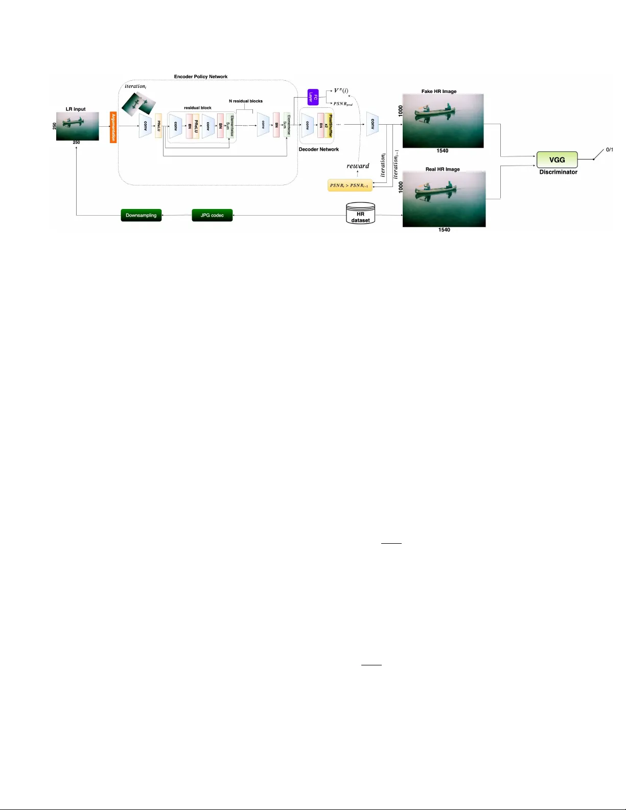
A Hybrid A ppr oach Between Adversarial Generativ e Networks and Actor -Critic P olicy Gradient f or Low Rate High-Resolution Image Compr ession Nicol ´ o Savioli Imperial College London, UK nsavioli@ic.ac.uk Abstract Image compr ession is an essential appr oach for de- cr easing the size in bytes of the image without deterio- rating the quality of it. T ypically , classic algorithms ar e used b ut r ecently deep-learning has been successfully ap- plied. In this work, is pr esented a deep super-r esolution work-flow for image compr ession that maps low-r esolution JPEG image to the high-r esolution. The pipeline consists of two components: first, an encoder-decoder neural net- work learns how to tr ansform the downsampling JPEG im- ages to high r esolution. Second, a combination between Generative Adversarial Networks (GANs) and r einforce- ment learning Actor -Critic (A3C) loss pushes the encoder- decoder to indir ectly maximize High P eak Signal-to-Noise Ratio (PSNR). Although PSNR is a fully differ entiable met- ric, this work opens the doors to new solutions for maxi- mizing non-differ ential metrics thr ough an end-to-end ap- pr oach between encoder -decoder networks and r einfor ce- ment learning policy gradient methods. 1. Introduction Image compression with deep learning systems is an ac- tiv e area of research that recently has becomes very com- pelling respect to the modern natural images codecs as JPEG2000, [1], BPG [2] W ebP currently dev eloped by Goog le R  [3]. The new deep learning methods are based on an auto-encoder architecture where the features maps, generate from a Con volutional Neural Networks (CNN) en- coder , are passed through a quantizer to create a binary rep- resentation of them, and subsequently given in input to a CNN decoder for the final reconstruction. In this vie w , sev- eral encoders and decoders models ha ve been suggested as a ResNet [4] style network with the parametric rectified linear units (PReLU) [5], generativ e approach b uild on GANs [6] or with a inno vati ve hybrid networks made with Gated Re- current Units (GR Us) and ResNet [7]. In contrast, this paper proposes a super -resolution approach, build on a modifying version of SRGAN [8], where downsampling JPEG images are con verted at High Resolution (HR) images. Hence, in order to improv e the final PSNR results, a Reinforcement Learning (RL) approach is used to indirectly maximize the PSNR function with an A3C policy [9] end-to-end joined with SRGAN. The main contributions of this works are: (i) Propose a compression pipeline based on JPEG image downsampling combined with a super-resolution deep net- work. (ii) Suggest a new way for maximizing not differen- tiable metrics through RL. Ho wev er , e ven if the PSNR met- ric is a fully dif ferentiable function, the proposed method could be used in future applications for non-euclidean dis- tance such as in the Dynamic Time W arping (DTW) algo- rithms [10]. 2. Methods In this section is given a more formal description of the suggested system which includes: the network architecture and the losses used for training. 2.1. Netw ork Ar chitecture The architecture consists of three main blocks: encoder , decoder and a discriminator (Figure 1). The I LR is the low- resolution (LR) input image (i.e compressed with a JPEG encoder) of size r W × r H × C ( i.e with C color chan- nels and W , H the image width and height); where a bicubic downsampling operation with factor r is applied. While the output is an HR image defined as I H R . 2.1.1 Encoder The encoder is basically a ResNet [4], where the first con vo- lution block has a kernel size of 9 × 9 and 64 Feature Maps (FM) with a P arametr icReLU activ ation function. Then, fiv e Residual Blocks (RB) are stacked together . Each of those RB consists of two con volution layers with kernel size 3 × 3 and 64 FM follo wed by Batch-Normalisation (BN) and P ar ametricR eLU . After that, a final con volution block of 3 × 3 and 64 FM are repeated. Ho wev er , the encoder is also 1 Figure 1: The figure sho ws the proposed RL-SRGAN model composed by encoder, decoder and discriminator networks. The objectiv e of this model is to map the compressed JPEG Low Resolution (LR) Image to the HR. The encoder can be seen as: (i) an RL policy network able to increase its HR prediction through the indirect maximization of the PSNR at each i training iterations. (ii) A GANs, where the discriminator (i.e V GG network) push the decoder to produce images similar to the original HR ground truth. joint with a fully connected layer and, at each i training it- erations, produces an action prediction of the actual PSNR; together with a v alue function V π ( I H R ( i )) (i.e explained in 2.2.2 section). 2.1.2 Decoder The decoder is fundamentally another deep network that al- lows increasing the resolution of the output encoder with eight subpixel layers [11]. 2.1.3 Discriminator The encoder , joint with the decoder , define a generator H ( · ) θ , where θ = [ w L ; b L ] are the weight and biases pa- rameters for each L-layers for the specific network. A third network D ( · ) θ , called discriminator , is also optimized con- currently with H ( · ) θ for solving the following adversarial min-max problem: l H R GAN = min θ max θ E I H R ∼ p train ( I H R ) [ log ( D ( I H R ))]+ + E I LR ∼ p H ( I LR ) [ log (1 − D ( H ( I LR )))] (1) The idea behind l H R GAN loss is to train a generati ve model H ( · ) θ to fool D ( · ) θ . Indeed, the discriminator is trained to distinguish super-resolution images I H R , generated by H ( · ) θ , from those of the training dataset. In this way , the discriminator is increasingly struggled to distinguish the I H R images (generated by H ( · ) θ ) from the real ones and consequently dri ving the generator to produce results closer to the HR training images. Then, in the proposed model, the discriminator D ( · ) θ is parameterized through a VGG net- work with Leak yReLU activ ation ( α = 0 . 2) without max- pooling. 2.2. Loss function The accurate definition of the loss function is crucial for the performance of the H ( · ) θ generator . Here, the para- graph is logically di vided into three losses: the SRGAN loss, the RL loss, and the proposed loss. 2.2.1 SRGAN loss The SRGAN loss is determined as a combination of three other separate losses: MSE loss, VGG loss, and GANs loss. Where the MSE loss is defined as: l H R M S E = 1 W H W X x =1 H X y =1 ( I H R x,y − H θ ( I LR ) x,y ) 2 (2) It represents the most utilized loss in super-resolution methods but remarkably sensiti ve to high-frequency peak with smooth textures [8] . For this reason, is used a VGG loss [8] based on the ReLU acti vation function of a 19 layer VGG (defined here as Ω( · ) ) network: l H R V GG = 1 W H W X x =1 H X y =1 (Ω( I H R ) x,y − Ω( H θ ( I LR ) x,y ) 2 (3) Where W and H are the dimension of I H R image in the MSE loss. Whilst, for the VGG loss, they are the Ω( · ) output FM dimensions. While the GANs loss is previously 2 defined in the equation 1. Finally , the total SRGAN loss is determined as: l H R S RGAN = l H R M S E + 1 e − 3 × l H R GAN + 6 e − 3 × l H R V GG (4) 2.2.2 RL loss The aim of RL loss is to indirectly maximize the PSNR through an actor -critic approach [9]. Giv en Q π ( I LR , P S N R pred ) a map between the low resolution in- put I LR and the current PSNR value prediction P S N R pred (see fig. 1). Thence, at each i training iterations, is calcu- lated the rew ard value as a threshold between the pre vious P S N R at iteration i − 1 and that one to iteration i as fol- lows: r ( i ) = ( 1 , if P S N R i > P S N R i − 1 0 , otherwise (5) where the P S N R ( · ) function is defined as: P S N R = 20 · log 10 ( M AX I ) − 10 · log 10 ( 1 mn m − 1 X l =0 n − 1 X j =0 [ I H R ( l, j ) − I H R g t ( l, j )] 2 ) (6) The M AX I is the maximum pixel value of the HR im- age, I H R is the output encoder HR image, while I H R g t is the corresponding HR ground truth for each pixel ( l, j ) at m × n HR size. The re ward (eq. 5), actually depends on the P S N R pred action taken by the policy for two main reasons: (i) during the training process the P S N R pred becomes an optimal estimator of the decoder output I H R (used in 6). (ii) The latent space between the encoder and the fully connected layer is the same and share equal policy information. Thus, all the re wards are accumulated e very k training steps through the following return function: R ( i ) = ∞ X k =0 γ k r ( i + k ) (7) where γ ∈ (0 , 1] is a discount factor . Therefore, is pos- sible to define the Q π ( · ) function as an e xpectation of R ( k ) giv en the input I LR and P S N R pred . Q π ( I LR , P S N R pred ) = E [ R ( i ) | I LR ( i ) = I LR , P S N R pred ] (8) T o notice, the encoder , together with the fully connected layer , become the policy network π ( P S N R pred | I LR ( i ); θ H ) . This policy network is parametrized by the standard RE I N F O RC E method on the θ encoder parameters with the following gradient direction: ∇ θ log π ( P S N R pred | I LR ( i ); θ ) · R ( i ) (9) It can be consider an unbiased estimation of ∇ θ · E [ R ( i )] . Especially , to reduce the variance of this e valuation (and keeping it unbiased) is desirable to subtract, from the return function, a baseline V ( I LR ( i )) called value function. The total policy agent gradient is gi ven by: l H R π = log π ( P S N R pred | I LR ( i ) , θ ) · ( R ( i ) − V ( I LR ( i ))) (10) Figure 2: The abov e figure shows the results for RL- SRGAN compared to SRGAN, LANCZOS, and the orig- inal ground truth. As we can see, LANCZOS simply de- stroys the edges producing artifacts on the global image. Whilst, SRGAN forms noticeable chromatic aberration (i.e transition from orange to yellow color) near the edges. Even though, the RL-SRGAN holds the color uniform with net outline details nearby to the edges; analogous to the origi- nal ground truth. The term R ( i ) − V ( I LR ( i )) can be considered a esti- mation of the advantage to predict P S N R pred for a giv en I LR ( i ) input. Consequently , a learnable ev aluation of the value function is used: V ( I LR ( i )) ≈ V π ( I LR ( i )) . This ap- proach, is further called generativ e actor-critic [9] becouse the P S N R pred prediction is the actor while the baseline V π ( I LR ( i )) is its critic. The RL loss is then calculated as: l H R RL = 5 e − 3 ∗ X ( R ( i ) − V π ( I LR ( i ))) 2 − l H R π (11) 2.2.3 Proposed loss The Proposed Loss (PL) combines both SRGAN loss and RL loss. After ev ery k step (i.e due to the rew ards accumu- lation process at each i training iterations), the l H R RL is added on l H R S RGAN . l H R P L = ( l H R S RGAN + l H R RL , if k = i l H R S RGAN , otherwise (12) 3 Methods PSNR MS-SSIM RL-SRGAN 22.34 0.783 SRGAN 22.15 0.780 LANCZOS 21.44 0.760 T able 1: The table shows the PSNR and MS-SSIM re- sults obtained in the v alidation set for the proposed rl-srgan method with srgan and lanczos upsampling. 2.3. Experiments and Results In this section is e v aluate the method suggested. The dataset used is the CLIC compression dataset [12] corre- spondingly divided in the train, valid and test sets. The train has 1634 HR images, valid 102 and test 330 . The ev aluation metrics used are the PSNR and MS-SSIM [13] for both valid and test. An AD AM optimizer is used with a learning rate of 1 e − 3 within 22876 model iterations until con vergence. The Reinforcement Learning SRGAN (RL- SRGAN) is compared with the SRGAN model work [8] and the Lanczos resampling (i.e a smooth interpolation through a con volution between the I LR image and a stretched sinc ( · ) function). Finally , the table 1 highlights that the PSNR difference between LANCZOS upsampling and RL- SRGAN is 0.9, while of 0.19 with SRGAN; whereas the MS-SSIM remains constant between RL-SRGAN and SR- GAN for the v alidation set. This also sho ws a better accu- racy for the RL-SRGAN model. While, for the tests, RL- SRGAN achie ve 20 . 06 of PSNR and 0 . 7503 of MS-SSIM. Furthermore, the compression rate for the v alidation set im- ages is 3.812.623 bytes respect 362.236.068 bytes of origi- nal HR dataset. While for the test set images is 5.228.411 bytes in contrast with the 5.882.850.012 bytes of the origi- nal one. That makes the method a good trade-off between compression capacity and acceptable PSNR. 2.4. Discussion A modified version of SRGAN is suggested where an A3C method is joined with GANs. Sadly , the proposed method has strong limitations due to the drastic downsam- pling of the input JPEG image. This do wnsampling causes loss of information, difficult to reco ver from the super- resolution network, which leads to lower results in PSNR and MS-SSIM on the test set (i.e 20 . 06 and 0 . 7503 re- spectiv ely). Despite, the results (table 1) emphasize slight improv ement performances for RL-SRGAN related within SRGAN and a baseline LANCZOS upsampling filter . How- ev er, the proposed method compresses all test files in a par - simonious way respect to the challenge methods. Indeed, the total dimension of the compression test set is of 5236870 bytes respect to 15748677 bytes of CLIC 2019 winner . Finally , a new method for maximizing non-differentiable functions is here suggested through deep reinforcement learning technique. References [1] David S. T aubman and Michael W . Marcellin. JPEG2000 : image compr ession fundamentals, standards, and practice / David S. T aubman, Michael W . Marcellin . Kluwer Academic Publishers Boston, 2002. [2] Fabrice bellard. bpg image format. https://bellard. org/bpg . [3] W ebp image format. https://developers.google. com/speed/webp . [4] Kaiming He, Xiangyu Zhang, Shaoqing Ren, and Jian Sun. Deep residual learning for image recognition. CoRR , abs/1512.03385, 2015. [5] Haojie Liu, T ong Chen, Qiu Shen, T ao Y ue, and Zhan Ma. Deep image compression via end-to-end learning. In The IEEE Conference on Computer V ision and P attern Recogni- tion (CVPR) W orkshops , June 2018. [6] Eirikur Agustsson, Michael Tschannen, Fabian Mentzer, Radu T imofte, and Luc V an Gool. Extreme learned image compression with gans. In The IEEE Conference on Com- puter V ision and P attern Recognition (CVPR) W orkshops , June 2018. [7] George T oderici, Damien V incent, Nick Johnston, Sung Jin Hwang, David Minnen, Joel Shor , and Michele Covell. Full resolution image compression with recurrent neural net- works. In The IEEE Confer ence on Computer V ision and P attern Recognition (CVPR) , July 2017. [8] Christian Ledig, Lucas Theis, Ferenc Huszar, Jose Caballero, Andrew Cunningham, Alejandro Acosta, Andrew P . Aitken, Alykhan T ejani, Johannes T otz, Zehan W ang, and W enzhe Shi. Photo-realistic single image super-resolution using a generativ e adversarial network. In 2017 IEEE Conference on Computer V ision and P attern Recognition, CVPR 2017, Honolulu, HI, USA, J uly 21-26, 2017 , pages 105–114, 2017. [9] V olodymyr Mnih, Adri ` a Puigdom ` enech Badia, Mehdi Mirza, Alex Graves, Timothy P . Lillicrap, Tim Harley , David Silver , and Koray Kavukcuoglu. Asynchronous methods for deep reinforcement learning. CoRR , abs/1602.01783, 2016. [10] Eamonn J. Keogh and Michael J. Pazzani. Scaling up dy- namic time warping for datamining applications. In Pro- ceedings of the Sixth ACM SIGKDD International Confer- ence on Knowledge Discovery and Data Mining , pages 285– 289. A CM, 2000. [11] Andrew P . Aitken, Christian Ledig, Lucas Theis, Jose Ca- ballero, Zehan W ang, and W enzhe Shi. Checkerboard ar- tifact free sub-pixel conv olution: A note on sub-pixel con- volution, resize con volution and con volution resize. CoRR , abs/1707.02937, 2017. [12] W orkshop and challenge on learned image compression (clic). http://www.compression.cc/ . [13] Zhou W ang, Eero P . Simoncelli, and Alan C. Bovik. Multi- scale structural similarity for image quality assessment. pages 1398–1402, 2003. 4