Modeling and Control of Combustion Phasing in Dual-Fuel Compression Ignition Engines

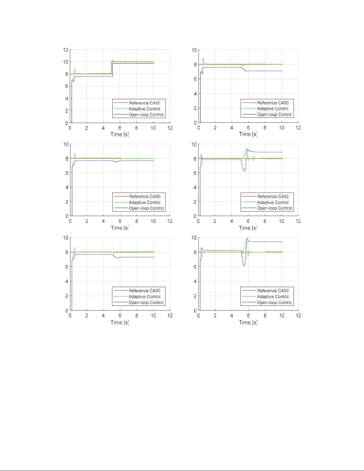
GTP- 18 -1 18 1 (H al l) 1 Modelling a nd Control of Combustion Phasing in Dual -Fuel Compression Igniti on Engines Wenbo Su i 1 , Jorge Pulpeiro Gon zález 1 and Ca rrie M. Hall 1 * 1: Illinois Institute of Technolog y Abstract: Dual fuel engines can achieve high efficiencies and low emissions b ut also can encounte r hi gh cylinder-to-cylinder v ariations on multi-c y linder eng ines. In order to avoid these v ariations, they require a more complex method for combustio n phasing control such as m odel-based control. Since the combustion process in these engines is complex, t ypical models of the system are complex as well and there is a need for sim pler, computa tionally efficient, control -oriented models of the du al fuel combust ion proce ss. In this pap er, a m ean-value combustion phasing model i s designed and calibrated and two control strategies are proposed. C ombustion phasing is predicted using a knock integral model, b urn du ration model and a Wiebe function and this model is used in both an adaptive closed loop cont roller and a n open loop controller. These two control methodologies are tested and compared in simula tions. Both control strategies are able to rea ch steady stat e in 5 cycles af ter a transien t and h ave stead y state e rrors in CA50 that are le ss than ±0.1 crank a ngle de gree (CA D) with the adapti ve co ntrol str ategy and l ess than ±1.5 CAD with the model-based feedforward c ontrol method. Keywords: Combustion phasing, dual fuel engine, model-ba sed control, adaptive control, combustion control Introduction In th e transportation area, re gulations continue to require low er emis sions whil e the m arket simultaneousl y demands higher fuel efficiencies. Thes e requirements ha ve led to ma ny new technological developm ents including vari able geometr y t urbocha rgers, va riable valve actuation systems and advanced exhaust aftertreat ment sy s tems. Dual-fuel c apabiliti es hav e also been explored and been shown to have the potent ial to increase efficie ncies while producing m uch lo wer emissions of nit rogen ox ides and pa rticulate matter than conventio nal diese l engines [1]. Dual fuel combustion strategies t ypically use two fuels with differ ent reac ti vities to cre ate in-c y linder reactivit y stratification that provi de greater cont rol of combustion phasing and pressure ris e rate [2]. These benefits of dual fuel eng in es have b een explored on single cy l inder [3] and multi- cylinder engines [ 4, 5, 6, 7, 8]. As with conventional internal combusti on en gines, optimal combustion phasing is critic al to ma intain high efficien cies o n dual fu el engines, and as such, control of this parameter is paramount [9, 10]. Due t o the increasingl y complex config uration of these engines, there is interest in using m odel- based control st rategies t o accu rately cont rol the e ngine process es including combustion pha sing. Combustion phasing on conventional diesel engines has b een captur ed usi ng a v ariet y of mo dels. In [11, 12, 13] , a model based on the Shell aut o-ignition method w as used to make precise prediction of th e st art of combustion (SOC), but this model requires a d etailed CFD analysis for GTP- 18 -1 18 1 (H al l) 2 calibration. The kno ck integral m odel (KIM), which was first proposed b y Livengood and Wu to predict the knock of a spark ignition eng ine [14] , has al s o been utilized to predict SOC [15,16,17] on diesel en gines. In [ 14], Hillio n et al . employed a KIM to predi ct SOC and t he end o f the cold flame. Other factors such as emissions including CO and NO mass flow rates have also been estimated using this model [15,16]. In addition, the KIM has been mo dified by Shahbakhti to include the impact of v arying air-fuel ratio and E GR fraction on SOC in a homogenous c harge compression ignition (HCCI) engine [18]. Different forms of the Arrhenius factor in the knock integral w ere also stu died in [19] in order to predict and control the SO C and location of pe ak pressure in a HCCI engin e. Efforts to expand t hese m odels to dual fuel compression ignition engines i nclude ex tensions of semi-empirical models such a s the Wie be functi on [20] and probabil ity densit y function (PDF) based m odels. In [ 21] and [ 22], a PDF based stochastic reactor model is leveraged to mo del th e combustion process of a dual-fu el H CCI engine and is experiment ally verified. This model characterizes the combustion process including chemical kinetics and inhomog eneous compositions and temperatures. Wi th this PDF based model, Bhave et al. a re able to e stimate SOC. In [23] , a single zone co mbustion model with det ailed chemical m echanism was su ccessfully used to obtain an accurate estimation of SOC for dual fuel engines. However, this model does not properly esti mate burn duration and has a high computation time. I n [ 20], the ignition delay of a dual fuel engine is captur ed, but other aspects of combustion phasing are not addressed. In contr ast, this work seeks to model the combustion phasing of a dual fu el engine including SOC and CA50. Combustion phasing control has been accomplished using traditi onal PID (Proportion Inte gral Derivative) controllers as well as unde rl y in g mod els a nd feedback from addit ional sensors. I n [24], a modified KIM m odel is simplified via an empirical correlation and an observer-based state- feedback controller i s impl emented to control SOC. I n [25], Olsson et al. proposed a closed-loop PID controller to achieve t he desi red C A50 with short response ti me i n a dual-fuel HCC I engin e. The PID gains w ere tuned based on a sensitivit y function that w as developed based o n the experimental data in a HCC I dual-fuel engine. A similar m ethod is inve stigated b y Maur ya et al. in [26] . A si mple PID controller was utiliz ed to control CA50 with pressure rise rate limitation based o n fuel blend ratio. Strandh et al. leveraged a P ID controller and a LQG (linear Quadratic Gaussian) controller to c ontrol C A50 base d on ion meas u rements and in-cylinder pr essure feedback [27]. Another PID controller based on discrete lineariz ed model was posted by Ott et al. in [28]. The controller adjusted the i njection time and duration of d iesel fuel for controlling the combustion phasing and t he max imum in-cylinder pres su re. In re fe rence [29] , three P I (Proportion Integral) controlle rs based on a map-based RCC I model were used to control the CA50 and the IMEP (indicated me an ef fective pressure). Kondi pati et al. ha ve utilized a PI controlle r to track the desired CA50 b y controlling the fuel mixture ratio and injection ti ming [30]. In order to reject the disturbance, a look-up table feedforward control ler was us ed a long with th e P I feedba ck controller. Unlike t hese prior stu dies, this work ex plores a sim plification to a m odified K I M model that ma kes it m ore s uitable for real-time control . I n this work SOC and CA50 are m odelled and two control approaches are dev eloped. Since combustion efficienc y is a strong fun ction of CA50, cont rol of these parameters are c ritical [ 31]. The m odel predic ts t he SOC u sing a m odified knock in tegral model (MK IM) and co m putes the burn durat ion (BD) using a separate bu rn durat ion model. C A50 GTP- 18 -1 18 1 (H al l) 3 is later calculated usin g these two parameters. Th e integral model is simplif ied into a non-linear model that is calibrated usi ng simulation data. An adaptive feedback controller is designed to control the CA50 b ased on this non-l inear model using a mea surement of CA50. Sim ulation results show that the combustion phasing can reach steady state in 10 cy cles after a transient and the steady s tate error in CA50 is less than ±0.1 CAD. Although th ere are som e commercial diesel en gines that have in-c ylinder sensors that could estimate CA50 values, other production engines do not. T hus, use of this control str ategy ma y be more limited. To overco me this disadvanta ge, an additional control stra tegy based on open-loop feedforward model-based control was develope d. This control technique can give an app ropriate start of injection (SO I) based on the simple non-linea r model. Simula tion results for this second control strateg y showed that CA50 settled to the steady state v alue in 10 cycles when the operating conditions were changed and the stead y state errors were less than ±1.5 CAD. The pap er describe s the combusti on phas in g prediction model. After the experimental and simulation setup are described, the model development and calibration procedure i s discussed as well as the development of the two different control strat e gies. Next, the results of the simulations are presented and anal y z ed. Finall y, some conclusions are made regarding the performance of the control techniques used in this work. Dual-Fuel Engine E xperimental and Simulatio n Model Setup Fig.1 shows the config u ration of the dual-fuel engine studied in thi s work. In this engine, am bi ent air is compressed (b y a compressor) and mix ed w ith recirculated exhaust gasses and a low reactivit y fuel in the intake manifold. After the intake stroke, a high reactivit y fuel is injected into the c ylinder and combust ion occurs. After the exhaust stroke, the bu rned gases go to the exhaus t manifold, where portion goes to the exhaust gas recirculation (E GR) flow path towards the intake manifold and the rest passes through the turbine, ge nerating the power n ecessar y to driv e the compressor. In th is work, natural gas was us ed as the low re activity fuel and diesel w as the hi gh reactivit y fuel . To calibrate the CA50 prediction model and evaluate its accurac y, it is compared to e xperimental results as well as simulation results from GT-ISE (Gamma Technolog y’s I nte grated Simula tion Environment). The simulation model used in this work has been previousl y used in [8] and [9] and is described briefly here. The en gine specifications are shown in T able 1. This sim ulation model was developed and v alidated based on 20 ex periments at d ifferent o perating points. I t uses bot h a direct-injectio n combustion model and traditional port-injection combustio n model to capture the dual fuel combusti on event. Results from 10 diesel onl y ex periments were used to properly calibrate direct-injection portion in the GT-ISE simulat ion model, and 10 dual fuel experiments with diesel and natural gas were use d to calibrate the port-injec tion portion [ 9]. This sim ulation model has a ±1.8 CAD uncertaint y compa red with expe rimental results and is used here t o simula te the com bustion process of the dual-fuel en gine over a w ide ran ge of oper ating points as sh own in Table 2. A total o f 1054 simulations at different op erating co n ditions w ere tested, and the coefficien ts in the CA50 model are calibrated usin g these simulations. GTP- 18 -1 18 1 (H al l) 4 Combustion Phasing Mode l A bl ock di agram of the combust ion phasing prediction model for dual-fu el engines is shown in Fig. 2 . This model contains thre e p arts: a SOC model, burn duration model and CA50 model. First, the SOC is predicted b y a modified knock int egral model based on t he SO I (start of diesel injection), pressure and temperature at IVC ( 𝑃  and 𝑇  ), engine speed ( 𝑁 ), and EGR f raction, as well as the equivalenc e ratios of diesel ( 𝜙  ) and n atural gas ( 𝜙  ). Meanwhile , the bur n duration (BD) m odel is estima ted based on the EGR fraction, residual gas fraction ( 𝑋  ), the diesel and natural gas equivalence ratios. Afterwards, the CA50 is predicted based on SOC and BD by a CA50 model developed from Wi ebe function. SOC Prediction M odel A KIM captures the relat ionship between IVC and SOC as  𝜏 𝑁   𝑑𝜃 = 1 (1) where IVC denotes intak e valve closing, SOC ind icates the start of combustion, N represents the engine speed, and 𝜏 denotes the Arrhenius function. The Arrhenius func tion can take different forms bu t is often a function of fuel equiva lence ratios, compression temperature and pressure. In this work, the Arrhenius function is given by 𝜏 = 1 ( 𝑎  𝐸𝐺𝑅 + 𝑎  ) 𝜙   exp  − 𝑎  𝑃   𝑇  (2) in which 𝐸𝐺𝑅 represents th e E GR fraction, 𝜙 is the fuel e quivalence ratio, T and P are the d ynamic temperature and pressure, and 𝑎  , 𝑎  , 𝑎  , 𝑎  and 𝑎  are the empirical constants. In this engine, natural gas is port-inject ed and d iesel is direct-inje cted. As such, the equival ence r atio term in Eqn. (2) is not cons tant in dual- fuel engines. Since diesel is i njected at SO I, the equivalence ratio term should have different forms from IVC to SO I and SOI to SOC. Therefore, th e Arrhenius function between IVC and SO I can be writt en as in Eqn. (3), and the Arrhenius func tion between SOI and SOC is captured b y Eqn. (4). 𝜏  = 1 ( 𝑏  𝐸𝐺𝑅 + 𝑏  ) 𝜙    exp 󰇧 − 𝑏  𝑃   𝑇 󰇨 (3) 𝜏  = 1 ( 𝑐  𝐸𝐺𝑅 + 𝑐  )  𝜙    + 𝜙     exp  − 𝑐  𝑃   𝑇  (4) Here 𝜙  is th e equivalence rati o of natura l g as and 𝜙  indicates the equivalence ratio of diesel, as defined in Eqns. (5) and (6), respectivel y. 𝜙  =  𝑚  𝑚   /  𝑚  𝑚    (5) 𝜙  =  𝑚  𝑚   /  𝑚  𝑚    (6) In these equations, 𝑚  and 𝑚  are th e natural gas injection mass and di esel inje ction mass each c ycle, and 𝑚  is the m ass of air ent ering in the engine c ylinder. The sub script 𝑠𝑡 indic ates stoichiometric conditions. GTP- 18 -1 18 1 (H al l) 5 Substituting Eqns. (3) and (4) into Eqn. (1), the K IM can be rewritten as  exp  − 𝑏  𝑃   𝑇  ( 𝑏  𝐸𝐺𝑅 + 𝑏  ) 𝑁 𝜙      𝑑𝜃 +  exp  − 𝑐  𝑃   𝑇  ( 𝑐  𝐸𝐺𝑅 + 𝑐  ) 𝑁  𝜙    + 𝜙       𝑑𝜃 = 1 (7) As de monstrated in [24] and confirmed in th is study, t he first integral te rm in Eqn. (7) is much smaller than t he s econd inte gral term in Eqn. (7), because th e activatio n energ y of na tural gas 𝑏  is much higher than the activatio n energy of the m ixture of the fuels 𝑐  [24, 32, 33] . A s such, t he exponential te rm in the se cond in tegral i s almost 10 9 time s as the exponenti al term i n the first integral and the first term can be ignored in the mod ified knock inte gral mode l of dual-fuel en gines. Even though the period from IVC to SO I is larger than the period from SOI to SOC, the first te rm in Eqn. (7) is neglectabl e. Therefore, the knock i ntegral model of dual-fuel engine SOC can be described by  exp  − 𝑐  𝑃   𝑇  ( 𝑐  𝐸𝐺𝑅 + 𝑐  ) 𝑁  𝜙    + 𝜙       𝑑𝜃 = 1 (8) It should b e noted that this knock inte gral model assumes that combustio n does not occur from IVC to SOC. During this process, wall heat losses are also i gnored from IVC to SO C as is typical in knock integral models [ 34]. Burn Duration Pred iction Mode l Burn duration is captured b y 𝐵𝐷 = 𝑐  ( 1 + 𝑋  )    𝜙    + 𝜙     (9) where 𝑋  represents the dilution fraction, 𝜙  and 𝜙  are t he equivalence ratios of natural gas and diesel, and 𝑐  , 𝑐  𝑐  and 𝑐  are constant parameters. The d ilution f raction 𝑋  will include both recirculated exhaust gas and residu als. As such, 𝑋  can be represented as 𝑋  = 𝐸𝐺𝑅 + 𝑋  (10) in which 𝐸𝐺𝑅 denotes the E GR fraction, a nd 𝑋  indicates the residual f raction. The residual fraction 𝑋  is defined b y 𝑋  = 𝑚  𝑚  + 𝑚  + 𝑚  + 𝑚  (11) where 𝑚  represents the ma ss of residual air in the cylinder f rom th e la st c ycle, 𝑚  is th e ma ss of air entering the c ylinder, 𝑚  denotes t he mass of rec irculated e xhaust gas, and 𝑚  and 𝑚  are ma ss of natural gas a nd diesel, respectivel y. With values or estimates of 𝐸𝐺𝑅 , 𝑋  and the equivalence ratios of fuels, the burn duratio n can be estimated. CA50 Predic tion Mode l Based on the prediction of SOC and BD, a Wiebe function can be emplo yed to predict fraction of fuel burned as 𝑥  ( 𝜃 ) = 1 − e xp 󰇧 − 𝑎  𝜃 − 𝑆𝑂𝐶 𝐵𝐷   󰇨 (12) GTP- 18 -1 18 1 (H al l) 6 where 𝜃 is the crank angle, 𝑥  indicates the mass fraction of burned fuel, 𝑆𝑂𝐶 represent s the timing of SOC in crank angle, 𝐵𝐷 denotes the burn duration in crank angle, and 𝑎 and 𝑏 are constant coefficients. CA50 can be calculated b y evalua ting Eqn. (12 ) when 𝑥  equals 0.5. Thus, Eqn. (12) can be w ritten as 0 . 5 = 1 − exp 󰇧 − 𝑎  𝐶𝐴 50 − 𝑆𝑂𝐶 𝐵𝐷   󰇨 (13) Rearranging, CA50 can be predicted b y 𝐶𝐴 50 = 𝑆𝑂𝐶 +  ln2 𝑎   /  𝐵𝐷 . (14) Substituting Eqn. (9) into Eqn. (14), CA50 can be captured by 𝐶𝐴 50 = 𝑆𝑂𝐶 + 𝑐  ( 1 + 𝑋  )    𝜙    + 𝜙     (15) in which 𝑐  is defined as 𝑐  =  𝑙𝑛 2 𝑎   /  𝑐  . (16) Using these submodels, SOC can be esti mated by Eqn. (8), and CA50 can be predicted b y Eqn. (15). CA50 Mod el Simplif icatio n Although SOC and CA50 can be predicted b y Eqns. (8) and (15), the integral model is still too complex for applicati on in th e t ypical control de sign. Therefore, it is necessary to simpl ify the integral model in Eq. (8) for further control design work. The model can be sim plified by assumin g that in one specific com bustion cycle, equivalence ratios, engine speed a s well as EGR fraction can be treated as c onstants. Wi th that assumpti on, the equivalen ce ratio, engine sp eed and EGR fraction terms can be tak en out from the integral term as reflect ed in Eqn. (17). 1 ( 𝑐  𝐸𝐺𝑅 + 𝑐  ) 𝑁  𝜙    + 𝜙      exp  − 𝑐  𝑃   𝑇    𝑑𝜃 = 1 (17) The dynamic pressures and temperatures in Eqn. (17) can be captured by a polytropic correlation, stemming from the press ure and temperature at IVC. Typically, to achieve the opti mal CA50 in dual-fuel engines, the SOI shoul d occur aro und -20° to 5° aTDC, and the S OC occurs from 1 – 10 CAD a fter SOI. Wi th such small crank angle chan ges from SOI to SOC , the cy linder volume d oes not c hange d ramaticall y du ring this period. Ther efore, the d ynamic pressures and temperatures f rom SO I to SOC can be treated as co n stant values during this per io d, and t hey can be replaced b y the pre ss ure and temp erature at SOI. Whil e this simplification wi ll result in a slight lo ss in ac curacy, it al lows the inte gral eq uation to be simp lified as 1 ( 𝑐  𝐸𝐺𝑅 + 𝑐  ) 𝑁  𝜙    + 𝜙     exp 󰇧 − 𝑐  𝑃    𝑇  󰇨 ( 𝑆𝑂𝐶 − 𝑆𝑂𝐼 ) = 1 (18) GTP- 18 -1 18 1 (H al l) 7 where 𝑃  and 𝑇  are the pressure and temperature at SOI and they can be derive d by 𝑃  = 𝑃   𝑉  𝑉     (19) and 𝑇  = 𝑇   𝑉  𝑉       . (20) SOC can be predicted b y rearranging Eqn. (18) as 𝑆𝑂𝐶 = 𝑆𝑂𝐼 + ( 𝑐  𝐸𝐺𝑅 + 𝑐  ) 𝑁  𝜙    + 𝜙     exp 󰇧 𝑐  𝑃    𝑇  󰇨 . (21) Substituting Eqn. (21) into Eqn. (15), CA50 can be captur ed by 𝐶 𝐴 50 = 𝑆𝑂𝐼 + ( 𝑐  𝐸𝐺𝑅 + 𝑐  ) 𝑁  𝜙    + 𝜙     exp 󰇧 𝑐  𝑃    𝑇  󰇨 + 𝑐  ( 1 + 𝑋  )    𝜙    + 𝜙     . (22) Thus, the CA50 in d ual-fuel engines can be predicted by Eqn. (22) with the SOI, EGR fra ction, engine speed, equivalence ratios of fu els, pressure and temperature at SO I and dilution fraction. CA50 Model Valida tion Calibration of CA50 Prediction Model GT-ISE simula tions were utilize d to calibrate the coefficients in the CA 50 prediction model. Th e time step of t hese simu lations is 0.1 CAD. The root mean square e rror ( RMSE) of CA50 was minimized by a batc h gradient des cent a lgorithm f or the CA50 prediction model based o n al l 1054 simulations. These simulations were tested at steady state. The model calibration procedure is shown in Fig. 3. First, a n initial guess of the parameters p rovided th e in itial conditio ns for the calibration and th e gradient of RMSE was set to zer o. For each simulation, th e CA50 was predict ed using t he CA50 model. After that, the R MSE and gradient of RMSE of this sim ulation were calculated. The RMSE and RMSE gradient of all si mulations was updated using t he gradient of RMSE of the current si mulation. After update, t he parameters were revised based on the R MSE gradient. The calibration i teration was stopped when the RMSE c ould no longer be decreased. The calibrated parameters of the CA50 prediction model in Eqn. (22) are given in Table 3. Validation of CA50 Prediction Mode l Based o n calibrated parameters in Tab le 3, the SOC and CA50 can b e predict ed by Eqns. (21) and (22). The predicted SOCs and CA50s are compared with the simu lation results in Fig. 4. In Fig. 4 (a), th e x axis is the SOC from the GT- ISE simulat ion, and the y axis is t he predicted SOC from Eqn. (21). The dashe d blue lines are ±1 C AD error limits. T he standard devi ation of the pred iction error is 0.2999 CAD, and the ma ximum error is 1.4852 CAD. GTP- 18 -1 18 1 (H al l) 8 Similarl y , Fig. 4 (b) c ompares the predicted CA 50 to the simulati on C A50 and the d ashed blu e lines are ±1 C AD error lim its. The standard deviat ion of the CA50 prediction error is 0.5317 CAD, and the max imum error is 2 .1902 CAD. Comparis on with Fig. 4 sh ows th at t he error of CA50 prediction is not only from errors in the predicti on of SOC, but also from inaccuracies in the prediction of B D. The err ors in the SOC prediction model are mainl y du e to the f act that h eat transfer was ignored from I VC to SOC. While these errors could be reduced with more compl ex models, the resu lts from Fig. 4 demonstrate t hat the E qns. (21) and (22) can predict SOC and CA50 with the error l ess than 1.5 CAD and 2.2 CAD, respe ctively. This is a sufficient le vel of accuracy to be us eful for dual-fuel engine combustion phasing control applications for the operating region parameteriz ed and errors in th is range should onl y have a minor impa ct on the th ermal efficiency of the engine. Ba sed on this C A50 prediction model, an adaptive feedback control strategy and a model-based open-loop control strategy w ere in vestigated. Note that this eng ine can experienc e cylinder-to-c y linder variations in CA50 pa rticularl y wh en la te IVC t im ings ar e used. M ore information on CA 50 variations in this dual fu el en gine can be found i n [36] . When high CA50 variations o ccur, more sophisticated control ap proaches ma y be required, b ut consideration of c ylinder-to-cylinder variations was outside the scope of this stu d y . Adaptive Fee dback Control Strateg y An adaptive control strategy was expected to provide precise CA50 control. However, thi s strategy requires some m ethod of CA50 feedback. Whi le this type of feedback is not common, it was investigated in this work to demons trate the usefulness of such an approach and provide a good reference with which to c ompare the simpler open loop method that will be dis cussed later. State-Space Model D erivation To design a n adaptive c ontroller dual -fuel engine combustion phasing control, a state- sp ace model is use d and is derived from the CA50 d ynamic model in Eqn. (22). In t his work, CA50 i s th e control reference 𝑦 , and the SOI is the control input 𝑢 . Thus, the state-s p ace model can be captured by 𝑦 = 𝑢 + 𝛼 𝑥  + 𝛽 𝑥  (23) in which 𝛼 = ( 𝑐  𝐸𝐺𝑅 + 𝑐  ) exp 󰇧 𝑐  𝑃    𝑇  󰇨 (24) 𝛽 = 𝑐  ( 1 + 𝑋  )   (25) 𝑥  = 𝑁  𝜙     + 𝜙     and (26) 𝑥  =  𝜙    + 𝜙     . (27) In t he CA50 state -space model s hown i n Eqns. (23) – (27), the s tates 𝑥  and 𝑥  change fro m cycle to cy cle and can b e computed fro m the eng in e speed and the equivalence ratios. The parameters 𝛼 GTP- 18 -1 18 1 (H al l) 9 and 𝛽 , which are influenced by 𝑃  , 𝑇  and dilution fraction 𝑋  , must be updated from cycl e to cycle. Adaptiv e Controlle r Design Based on the CA50 state-space model, an adaptiv e controll er was d esigned and a block diagram of the control strateg y is shown in Fig. 5. As shown in Fig. 5, the optimal CA 50 serves as the reference input for the controller. Measurements or estima tes of the engine sp eed and equivalen ce ratio of eac h fuel are use d to calculate the states with Eqns . (26) and (27) . Based on the referenc e CA5 0 and t he states, the adaptive c ontroller gives the appropriate SO I to engine c ontrol unit (ECU) for the diesel injection. The actual CA 50 is s ent back to the adaptive cont roller as the feedback to update t he paramet ers 𝛼 and 𝛽 in Eqns. (24) and (25). Using th e CA 50 pre d iction model in Eqn. (23), the appropriat e SOI (𝑢 ) can be found bas ed on the parameters 𝛼 and 𝛽 , states 𝑥  and 𝑥  and the reference output 𝑦  (the de sired CA 50). Rewritin g Eqn. (23), the input 𝑢 c an be given as 𝑢 = 𝑦  − 𝛼 𝑥  − 𝛽 𝑥  . (28) Since the pa rameters 𝛼 and 𝛽 va ry from c ycle to c ycle and i nclude unmeasured parameters ( 𝑃  , 𝑇  and dilution fraction 𝑋  ), the controller c an only calc ulate 𝑢 based o n estimated values rather than the actual values of 𝛼 and 𝛽 . Repl acing the actual values of 𝛼 and 𝛽 by th e observed values 𝛼  and 𝛽  , Eqn. (28) can be writte n as 𝑢 = 𝑦  − 𝛼  𝑥  − 𝛽  𝑥  . (29) To ensure ac curate obse rved values o f pa rameters 𝛼 and 𝛽 , an observer is designed based on gradient descend al gorithm. T he error function i s defined as the root mean squared error (RMSE) of the CA50, and it is given by 𝐸 = 1 2 ( 𝑦 − 𝑦  )  (30) where 𝐸 ex presses the R MSE, 𝑦 is the actual output and 𝑦  represents the observed out put. The observed output 𝑦  can be captured by 𝑦  = 𝑢 + 𝛼  𝑥  + 𝛽  𝑥  . (31) Comparison of Eqn. (31) and Eqn. (29) shows that i f the input 𝑢 and the estimated parameters 𝛼  and 𝛽  are constants in stead y stat e, the estimated ou tput 𝑦  should be the same as the desired output 𝑦  . Thus, Eqn. (30) can be rewritten b y re pl acin g 𝑦  b y 𝑦  as 𝐸 = 1 2 ( 𝑦 − 𝑦  )  . (32) With the error function in Eqn. (32), the partial derivatives of the observed parameters are 𝜕𝐸 𝜕 𝛼  = − 𝑥  ( 𝑦 − 𝑦  ) (33) 𝜕𝐸 𝜕 𝛽  = − 𝑥  ( 𝑦 − 𝑦  ) . (34) GTP- 18 -1 18 1 (H al l) 10 With the gradient desc ent algorithm, th e observed param eters 𝛼  and 𝛽  can be updated from cycle to cycle b y following equations 𝛼  ( 𝑘 + 1 ) = 𝛼  ( 𝑘 ) − 𝜂 𝜕𝐸 𝜕 𝛼  (35) 𝛽  ( 𝑘 + 1 ) = 𝛽  ( 𝑘 ) − 𝜂 𝜕𝐸 𝜕 𝛽  (36) where 𝛼  ( 𝑘 + 1 ) , 𝛽  ( 𝑘 + 1 ) , 𝛼  ( 𝑘 ) and 𝛽  ( 𝑘 ) are th e o b served p arameters at the 𝑘 + 1 cycle and 𝑘 cycle, respectivel y; 𝜂 indicates t he learnin g rate of the algorithm; and    and     are t he gradients given in Eqns. (33) and (34). Substituting (33) into (35) and substituti ng (34) into (36), the paramete r update equations are 𝛼  ( 𝑘 + 1 ) = 𝛼  ( 𝑘 ) + 𝜂 𝑥  ( 𝑦 − 𝑦  ) (37) 𝛽  ( 𝑘 + 1 ) = 𝛽  ( 𝑘 ) + 𝜂 𝑥  ( 𝑦 − 𝑦  ) . (38) In this work, the learning rate 𝜂 is 𝜂 = 1 𝑥   + 𝑥   . (39) The lea r ning rate 𝜂 in Eqn. (39) is chosen to achieve s ystem sta bility, sh ort set tling time and small overshoot. Substituting Eqn. (39) into Eqns. (37 ) and (38), th e update equations for the observed param eters are 𝛼  ( 𝑘 + 1 ) = 𝛼  ( 𝑘 ) + 𝑥  𝑥   + 𝑥   ( 𝑦 − 𝑦  ) (40) 𝛽  ( 𝑘 + 1 ) = 𝛽  ( 𝑘 ) + 𝑥  𝑥   + 𝑥   ( 𝑦 − 𝑦  ) . (41) Eqns. (29), (40) and (41) summarize t he adapti ve feedba ck cont rol s ystem t hat can be used to track the desired CA50. Adaptiv e Control Syste m Stabilit y The stability of th e adapt ive control s ystem should be guaranteed b efore practical a pplication in dual-fuel engines. A Ly a punov direct method is ut ilized to prove the stabil ity of the strat eg y. Since the goal of the c ontrol sy s tem is to minimize the error between th e actual CA50 and desired CA50, the Lyapunov function is chosen as 𝑉 [ 𝑥 ( 𝑘 ) ] = ( 𝑦  − 𝑦 )  . (42) For this chosen Lyapunov function, i t can be shown that 󰇱 𝑉 [ 𝑥 ( 𝑘 ) ] = 0 , if 𝑦  − 𝑦 = 0 , 𝑉 [ 𝑥 ( 𝑘 ) ] > 0 , ∀ 𝑦  − 𝑦 ≠ 0 and 𝑉 [ 𝑥 ( 𝑘 ) ] → ∞ , if 𝑦  − 𝑦 → ∞ . (43) Substituting Eqns. (23) and (29) into Eqn. (42), the Lyapunov function can be captured b y: GTP- 18 -1 18 1 (H al l) 11 𝑉 [ 𝑥 ( 𝑘 ) ] = 󰇣 𝑥   𝛼 ( 𝑘 ) − 𝛼  ( 𝑘 )  + 𝑥  󰇡 𝛽 ( 𝑘 ) − 𝛽  ( 𝑘 ) 󰇢 󰇤  (44) To simplif y Eqn. (44), the observer errors are desc ribed as 𝛼  ( 𝑘 ) = 𝛼 ( 𝑘 ) − 𝛼  ( 𝑘 ) (45) 𝛽  ( 𝑘 ) = 𝛽 ( 𝑘 ) − 𝛽  ( 𝑘 ) (46) Substituting Eqns. (45) and (46) into Eqn. (44), the Lyapunov function can be rewritt en as 𝑉 [ 𝑥 ( 𝑘 ) ] =  𝑥  𝛼  ( 𝑘 ) + 𝑥  𝛽  ( 𝑘 )   . (47) Similar to Eqn. (47), Lyapunov function at the 𝑘 + 1 cycle can be c aptured by 𝑉 [ 𝑥 ( 𝑘 + 1 ) ] =  𝑥  𝛼  ( 𝑘 + 1 ) + 𝑥  𝛽  ( 𝑘 + 1 )   (48) where 𝛼  ( 𝑘 + 1 ) = 𝛼 ( 𝑘 + 1 ) − 𝛼  ( 𝑘 + 1 ) (49) 𝛽  ( 𝑘 + 1 ) = 𝛽 ( 𝑘 + 1 ) − 𝛽  ( 𝑘 + 1 ) . (50) Substituting Eqns. ( 40) and (41) in to Eqns. (49) and (50) respectivel y, the errors of parame ters observation at 𝑘 + 1 cycle can be given b y Eqns. (51) - (52). 𝛼  ( 𝑘 + 1 ) = 𝛼 ( 𝑘 + 1 ) − 𝛼  ( 𝑘 ) − 𝑥  𝑥   + 𝑥   ( 𝑦 − 𝑦  ) (51) 𝛽  ( 𝑘 + 1 ) = 𝛽 ( 𝑘 + 1 ) − 𝛽  ( 𝑘 ) − 𝑥  𝑥   + 𝑥   ( 𝑦 − 𝑦  ) (52) Subtracting Eqn. (29) from Eqn. (23) y i elds 𝑦 − 𝑦  = 𝑥   𝛼 ( 𝑘 ) − 𝛼  ( 𝑘 )  + 𝑥  󰇡 𝛽 ( 𝑘 ) − 𝛽  ( 𝑘 ) 󰇢 . (53) Because the observed ou tput 𝑦  and desired 𝑦  are t he same in stead y state, 𝑦  ca n be repl aced b y 𝑦  in Eqn. (53) giving 𝑦 − 𝑦  = 𝑥   𝛼 ( 𝑘 ) − 𝛼  ( 𝑘 )  + 𝑥  󰇡 𝛽 ( 𝑘 ) − 𝛽  ( 𝑘 ) 󰇢 . (54) Substituting Eqns. (45) and (46) into Eqn. (54), it can be written as 𝑦 − 𝑦  = 𝑥  𝛼  ( 𝑘 ) + 𝑥  𝛽  ( 𝑘 ) . (55) The observat ion er rors at the 𝑘 + 1 cycle ca n be capt ured by substituting Eqn. (55) into Eqns. (51) and (52) resulting in 𝛼  ( 𝑘 + 1 ) = 𝛼 ( 𝑘 + 1 ) − 𝛼  ( 𝑘 ) − 𝑥  𝑥   + 𝑥    𝑥  𝛼  ( 𝑘 ) + 𝑥  𝛽  ( 𝑘 )  (56) 𝛽  ( 𝑘 + 1 ) = 𝛽 ( 𝑘 + 1 ) − 𝛽  ( 𝑘 ) − 𝑥  𝑥   + 𝑥    𝑥  𝛼  ( 𝑘 ) + 𝑥  𝛽  ( 𝑘 )  . (57) Since the parameters 𝛼 and 𝛽 are constant during stead y state, 𝛼 ( 𝑘 + 1 ) = 𝛼 ( 𝑘 ) and (58) 𝛽 ( 𝑘 + 1 ) = 𝛽 ( 𝑘 ) . (59) GTP- 18 -1 18 1 (H al l) 12 Substituting Eqns. (58) and (59) into Eqns. (56) and (57) respe ctively, the parameter observation errors are 𝛼  ( 𝑘 + 1 ) = 𝛼 ( 𝑘 ) − 𝛼  ( 𝑘 ) − 𝑥  𝑥   + 𝑥    𝑥  𝛼  ( 𝑘 ) + 𝑥  𝛽  ( 𝑘 )  (60) 𝛽  ( 𝑘 + 1 ) = 𝛽 ( 𝑘 ) − 𝛽  ( 𝑘 ) − 𝑥  𝑥   + 𝑥    𝑥  𝛼  ( 𝑘 ) + 𝑥  𝛽  ( 𝑘 )  . (61) Substituting Eqns. (45) and (46) into Eqns. (60) and (61), these equa tions can be simplified to 𝛼  ( 𝑘 + 1 ) = 𝛼  ( 𝑘 ) − 𝑥  𝑥   + 𝑥    𝑥  𝛼  ( 𝑘 ) + 𝑥  𝛽  ( 𝑘 )  (62) 𝛽  ( 𝑘 + 1 ) = 𝛽  ( 𝑘 ) − 𝑥  𝑥   + 𝑥    𝑥  𝛼  ( 𝑘 ) + 𝑥  𝛽  ( 𝑘 )  . (63) Further substituting Eqns. (62) and (63) i nto Eqn. (48), t he Lyapunov fun ction at the 𝑘 + 1 cycle is given b y Eqn. (6 4 ). 𝑉 [ 𝑥 ( 𝑘 + 1 )] = ⎣ ⎢ ⎢ ⎢ ⎢ ⎡ 𝑥   𝛼  ( 𝑘 ) − 𝑥  𝑥   + 𝑥    𝑥  𝛼  ( 𝑘 ) + 𝑥  𝛽  ( 𝑘 )   + 𝑥   𝛽  ( 𝑘 ) − 𝑥  𝑥   + 𝑥    𝑥  𝛼  ( 𝑘 ) + 𝑥  𝛽  ( 𝑘 )   ⎦ ⎥ ⎥ ⎥ ⎥ ⎤  (64) Simplif y in g Eqn. (64) at ste ady state, it can be found that 𝑉 [ 𝑥 ( 𝑘 + 1 ) ] = 0 . (65) Therefore, the difference between the Lyapunov function at the 𝑘 + 1 c ycle and the 𝑘 c ycle is captured in Eqn. (66). 𝑉 [ 𝑥 ( 𝑘 + 1 ) ] − 𝑉 [ 𝑥 ( 𝑘 ) ] = − ( 𝑦  − 𝑦 )  (66) According to Eqn. (66), the difference between t he Lyapunov function at the 𝑘 + 1 cycle and 𝑘 cycle is negative if 𝑦  − 𝑦 is not zero. Summarizing Eqn. (66) and Eqn. (43), it can be co nclud ed that ⎩ ⎨ ⎧ 𝑉 [ 𝑥 ( 𝑘 ) ] = 0 , if 𝑦  − 𝑦 = 0 , 𝑉 [ 𝑥 ( 𝑘 ) ] > 0 , ∀ 𝑦  − 𝑦 ≠ 0 , 𝑉 [ 𝑥 ( 𝑘 ) ] → ∞ , if 𝑦  − 𝑦 → ∞ and 𝑉 [ 𝑥 ( 𝑘 + 1 ) ] − 𝑉 [ 𝑥 ( 𝑘 ) ] < 0 , ∀ 𝑦  − 𝑦 ≠ 0 . (67) According to the Lyapunov direct method [35], th e outp ut of combustion phasing control s ystem is globally asymptotically stable. Feedforwa rd Model-based Controll er Design Because in-cylinder pressure sensors, which can provide CA50 estimates, are not common on production engines, t he adapti ve feedback control strategy ma y b e challenging. Fo r dual-fuel engines without CA50 m easurement, a mo del-base d op en-loop cont roller could still be applied. Such a co n troller is designed here to co ntr ol combustion phasing b y leveraging the dual fuel CA50 model. The block diagram of such a control s ystem is shown in Fig. 6. GTP- 18 -1 18 1 (H al l) 13 The reference CA50 i s still the reference input. The appropriat e SOI is c alculated b y a model- based o pen-loop controller with the reference inp ut and the engine paramet ers inclu ding e ngine speed, equivalen ce r atios, EGR fraction, pressure and t emperature at IVC. Using th e CA 50 prediction model shown in Eqn. (26), the SOI can be determined by 𝑆𝑂𝐼 = 𝐶𝐴 50  − ( 𝑐  𝐸𝐺𝑅 + 𝑐  ) 𝑁  𝜙    + 𝜙     exp 󰇧 𝑐  𝑃    𝑇  󰇨 − 𝑐  ( 1 + 𝑋  )    𝜙    + 𝜙     (68) in whic h 𝐶𝐴50  is th e reference CA50. Engine speed ( 𝑁) is t y pi call y available on production ECUs, and the eq u ivale nce ratios of fuels 𝜙  and 𝜙  can be calcul ated b y Eq ns. (5) and (6). EGR fraction (𝐸𝐺𝑅 ) can be esti mated based on the oxygen fr action at the intake and exhaust manifold as 𝐸𝐺𝑅 = 𝑥   ,   − 𝑥   ,   𝑥   ,  − 𝑥   ,  × 100% (69) where 𝑥 , , 𝑥 , , 𝑥 , are the oxygen fractions of ambient air, a t the intake m anifold and at the exhaust manifold. If ox ygen se nsors are not available i n the intake and ex haust manifolds, EGR flow can be estimated using methods such as those presented in [37]. Besides these me asurable pa rameters, the d ilution fraction ( 𝑋  ) and the pressure and t emperature at SO I ( 𝑃  and 𝑇  ) cannot be measured directl y from the sensors. Eqns. (19) and ( 20) can b e used to derive 𝑃  and 𝑇  from the pressure and te mperature at IVC ( 𝑃  and 𝑇  ). This I VC pressure a nd temperatur e ca n be esti mated bas ed on measured intak e man ifold conditions or a direct measurem ent c an be used. I n this w ork, measured val ues of 𝑃  and 𝑇  are levera ged. Substituting Eqns. (19) and (20) into Eqn. (68), the SOI can be captured b y 𝑆𝑂𝐼 = 𝐶𝐴50  − (𝑐  𝐸𝐺𝑅 + 𝑐  )𝑁 𝜙    + 𝜙     exp ⎣ ⎢ ⎢ ⎢ ⎡ 𝑐  󰇩 𝑃  󰇡 𝑉  𝑉  󰇢   󰇪   𝑇  󰇡 𝑉  𝑉  󰇢    ⎦ ⎥ ⎥ ⎥ ⎤ − 𝑐  ( 1 + 𝑋  )    𝜙    + 𝜙     (70) where 𝑉  is the volume of cy linder at SOI. Si nce the cylinder volume at a particular crank angle is known, 𝑉  can be found for a particula r choice of SO I. However, if 𝑉  is left in Eqn. (70), the control la w would need to com plete s everal iterations to compute the ap p ropriate SOI. T o decrease the co m putatio n procedure o f the contr ol st rategy, the 𝑉  from the prev i ous c ycle is used. Meanwhile, the dilution fraction 𝑋  can be computed based on EGR fraction and residual gas fraction 𝑋  in Eqn. (10). Whil e a variet y of m ethods exist for estimating EGR fraction, the re sidual gas fr action 𝑋  cannot be me asured directl y and i s difficult t o estimate. The value of 𝑋  ranges from 0.02 t o 0.05 fo r the conditions considered in this work and has much le ss variation th an t he EGR fractio n. As s uch, it is reasonable to use the average value of 𝑋   ( 𝑋   = 0.0329 ) to calculate SOI. Note th at if conditions such as positive valve overlap were considere d, 𝑋  c ould be much larger a nd ma y n eed to be separate ly modeled. Thus, the m odel-based o pen-loop control law is given by GTP- 18 -1 18 1 (H al l) 14 𝑆𝑂𝐼 = 𝐶𝐴50  − (𝑐  𝐸𝐺𝑅 + 𝑐  )𝑁 𝜙    + 𝜙     exp ⎣ ⎢ ⎢ ⎢ ⎡ 𝑐  󰇩 𝑃  󰇡 𝑉  𝑉  󰇢   󰇪   𝑇  󰇡 𝑉  𝑉  󰇢    ⎦ ⎥ ⎥ ⎥ ⎤ − 𝑐  ( 1 + 𝐸𝐺𝑅 + 𝑋   )    𝜙    + 𝜙     (71) The model-based open-loop controller will use Eq. (71) to g enerate an appro priate SO I in an effort to track the desired CA50. Simulatio n and Analysis I n this section, the two c ontrol lers bas ed o n adaptive feedback contro l and m odel pred ictive contro l are evaluated in simulations. Eac h te st will consider changes fr om one steady state point to another and six differ ent cases will be considered . In these simulations , the precision of SOI is set as 0.1 CAD. The deta iled set tings fo r a ll si x Cases are li sted in the Appen dix, whi le the simulation results are p lotted in Fig. 7. In the fi rst case, t he cont rollers’ performa nce is evaluated during a change in r eference CA50. Figure 7( a) shows the performance of both control algorithms duri n g t his change. In F ig. 7 (a), the red c urve is the referenc e CA50, and the green and blue line s a re t he actual CA50 achieved w ith adaptive control and open-loop control, respec tivel y. Fuel w as not injected into the sy stem in first 2 cy c les so the CA50s in those 2 cy cl es are zer o. In the first 5 seco n ds, both c ontrol systems rea ch their stead y states i n 5 cycles. The adaptive controller has a 0.8 CAD ov ershoot, and t he stead y state error v aries from -0.075 to 0.035 CAD dur ing stead y st ate. This os cillation of the e rror is mainly from the assumed precision limi tations of the injection rather than the control algorithm. In contrast, the op en-loop controll er has a -0.42 CAD steady sta te error without overshoot. The open-loop controller does not have such overshoot because it d oes not have a feedback iteration. When the re f erence CA50 is cha nged, the act ual CA50 is c hanged a cy cle later beca use of the reference CA50 samplin g method. At 5 seconds, the refe r ence CA50 is still 8 CAD, a nd it ha s changed into 10 CAD at 5.001 seconds. Because the contr oller has already receive d the reference CA50 and ca lc ulated the SOI before the new reference CA50 is generated , th e actua l CA50 has a one cycle delay . After the transien t , the C A50 from the adapti ve control case reaches steady st ate in 2 cycles with a 0.27 CAD over shoot, and the steady state error is fr o m -0.1 to 0.04 CA D. The open-lo op contr oller does not have ove rshoot, an d the steady state error i s -0.30 CAD . Next, the capabilit y of th e controlle rs to maintain the desir ed CA50 duri ng an en gine sp eed chan ge was explored. The simulation result is plotted in Fig. 7 (b). As ment ioned before, the fuel does not go into the s ystem in th e first 2 cycles, whic h l eads to zero C A50 in the first 2 cycles. In the first 5 seconds, both c ontrol s ystems c an reach th eir st eady states in 5 c ycles. The overshoot in th e adaptive control s ystem is 0.801 C AD. The steady state error mainl y from the SO I precision is - 0.073 – 0.030 CAD. D iffer ent from adaptive cont roller, the st eady s tate in the open-loop control system is -0.420 CAD. After 5 seconds , the engine speed inc reases smoothl y from 1200 RPM to 1500 RPM in 0.5 second. Both control strategies have reached th eir stead y s tate in 2 cycles after the transient. The stead y state errors are -0.033 – 0.077 CAD and -0.912 C AD in adaptive control system and open-loop control sy stem, respectivel y. The hig her steady state error in open-loop control system at the second operatin g condition is due to higher prediction error in the model. GTP- 18 -1 18 1 (H al l) 15 I n Ca se 3, the influence of a change i n the natural gas equivalence rati o is evaluate d by runnin g simulati on. Since the in fluen c e from natural gas equivale nce ra tio is similar with the effect by diesel equivalence ratio, only the equivalence ra tio of natural gas is shown here. During the firs t 5 seconds, the error is fairly low with only a steady state error of -0.031 to 0.071 CAD with adaptive control system and -0.33 CAD steady state error with open-loop contro l. Dur in g the transient , the natura l gas equ i valence ratio moves f rom 0.3 t o 0.5 i n 0.5 second. The i ncreasing equivalence ratio means that more natural gas has been mixed w ith the i nt ake air. During the transient, the residual gas fraction and the EGR compos iti on change due t o the chan ge of na tural g as quan tity . These changes also lead to changes in the intake gas proper ties, including the pressure and temperature at IVC. Despite this, good perfor m ance is seen with both controllers. Afte r the tran sient, th e CA 50s from both s y ste ms take about 5 c y cle s to reach the new steady states but have errors of -0.103 to 0.004 CAD with adaptive co nt rol and -0.328 CAD with the o pen-loop s trategy . As operating conditions change, EGR fraction may also be ex pected to change quite dramaticall y and the impact o f this is explo red in Case 4 . T he simula tion results are given in Fi g. 7 (d), respectively. Stead y state errors prior to th e transie nt at 5 seconds are lo w at -0.074 – 0.040 CAD for ad aptive cont rol and -0.167 CAD for open-loo p control. The EGR fraction changes f rom 0 to 0.5 during a 0.5 se cond ramp beginnin g at th e 5 se cond m ark and this leads t o significant errors initiall y with both controllers. Since the air handling system t ypicall y is not capable of abrupt changes, this r amp is closer to the actual performan ce of th e engine, but yet is stil l a very aggressive change. As shown in Eqns. (23) - (25), the EGR fraction is trea ted as a dis turbance term in the adaptive control s ystem. Thus, it takes about 10 cycles for the a daptive controlle r adjust to the ramp change in E GR fractio n. After a 1.332 CA D overshoot from 5.7 to 5.8 seconds, the actual CA50 backs to a stead y sta te around 8 CAD in 10 cy c les. Unlike the adaptiv e controller, the CA50 with open-loop control decreases from 5 to 5.5 second with its lowest value 6.25 CA D, and then jumps to a high of 9.20 CAD at 5 .9 seconds. This significant va riation i s related to the dela yed effect of the E GR fracti on change. The intake gas properties as well as the quantit y of fuel in jected change as a r esult of t he EGR fraction change. However, th ese changes ar e several c ycles later than the changes in EGR fraction. Because the EGR fraction values are directly used in the model leveraged b y the op en-loop control strateg y, the d ela y caus es mo re error du ring the tra nsient. After the transient, the s tead y state error is again low and ranges f rom -0.058 CAD to 0.045 CAD with adaptive control system and is 0.875 CA D with open-loop control. As in Ca se 5, a combine d change in cluding a ra mp in natural gas equiva lence ratio and engine speed is tested . The results are captured in Figure 6 (e). Similar to Case 2 and Case 3, CA50 in the adaptive control s ystem achieves its ste ady state in 5 cycles with an ove rshoot 0.603 CAD. The steady state erro r is from -0.033 to 0.072 CAD. Meanwhile, the open-loop control system has an error -0.332 CAD. From 5 to 5.5 seconds, both engine speed and natural gas equivalence ratio are ramped to their s econd value. In the transient, the engine speed increases from 1200 RPM to 1500 RPM, and the equivalence ratio of natural gas goe s from 0.3 to 0.5. Th ese ramp changes cause a slightly oscillation for the adaptive control s ystem. The CA50 in the open-loop s ystem moved from 7.669 to 7.307 CAD du ring the transient with the max imum erro r is -0.836 CAD. B oth controllers can re ach st eady state conditions at the second operating point before t he 6 second mark. The steady states error o f ad aptiv e controller and op en-loop controller are -0.063 to 0.046 CAD and 0.693 CAD, respectively. GTP- 18 -1 18 1 (H al l) 16 A second combined change was considered fo r Case 6. I n Case 6, EGR fraction changes along with engine speed and natura l gas equiv alence rati o. Thi s case is essentially a combination of Case 4 and C ase 5 and as such , the error a lso appea rs to be primarily an additio n of the error in Cas e 4 and Case 5. I n the first operating condition before 5 se cond, t he ste ad y state error of adaptive control s ystem is from -0.026 to 0.079 CAD, while th is error is 0.242 CAD for the open-loop control sy stem. From 5 to 5.5 second, the engine s peed, natural gas equivalen ce ratio and the EGR fraction wer e changed s moothl y in ramp. The performanc e du ring th is transi ent is s imilar to that of Case 4. The CA50 achieved with the adapti ve controller r eaches its pe ak value of 9. 521 C AD at 5.7 second and goes back to stead y state after. In the open -loop co ntr ol sy s tem, the CA50 drops to a minim um of 6.08 CAD at 5.4 se cond and j umps to a maximum value of 9.90 CAD at 5.8 seconds. As explained in Case 4, d ela ys in th e air h andling s ystem cause hi gher m odel errors. After the transient, the s tead y state er ror in ad aptive control system is -0.049 to 0. 032, while the open - loop controller h as a steady state er ror is 1.394 CAD. Comparison wi th Case 4 shows that the main error in Case 6 is likel y from the change in EGR fraction. These simulation s show that both contro llers can r eac h steady sta te quickly with a maximum steady state error less than ±0.1 C AD for adaptive con trol, and ±1.5 CAD for open-loop control. Still, both contro l lers cannot track the d esired C A50 as well when the para m eters of the engine change abrupt l y. This is especia lly significant in Case 4 an d Ca se 6, wh i ch has a large EGR fraction change in onl y 0.5 second. However , su ch a big, sudden change does not t ypical l y happen in norma l engine opera tion and Case 6 simply shows a worst-ca se scenari o. As expecte d, the a da ptiv e control le r is more accura te that the op en loop one , since it has a feed back signal , but since C A 50 me asureme nts are not available in most c ommerc ia l diesel engine s, the open-loop controller cou ld be more w idely used in stock diesel engines. Besides these o pera tin g condition s change s , the m easureme nts error is anothe r source whic h would h ighly influenc e on the contro ller perfor m ance . Discussion of Mea surement Errors Because the performa nce of the contro lle rs is highly dependent on sensor measure m ent s, measuremen t errors c ould significan t ly impact performance . The infl uence of the sensor measuremen t error s on the performance of contr ollers is studied in this section . Fir st, the error response of the open-loo p contro ller is i nvestiga ted. Meanwh il e, the adaptive control le r is tested with CA50 measurem ents error in the simulatio n. After these tests, the impact of the anticipat ed errors in CA50 on the combus tion efficiency is also d iscussed. For such an open-loop model-ba sed contr oller, measure m ent uncertai nty including measure ments errors , noise and cy clic variat ions will highly impact the control errors. To investigat e this, the CA50 prediction error from 𝑃  , 𝑇  , EGR fraction, f uel equ ivalence rati os an d 𝑋  have be en studied. A semi-empir ical m odel of 𝑃  and 𝑇  is present ed in [47], a nd t he uncertaintie s of 𝑃  and 𝑇  predic tion er ror are ±0.036 ba r and ±3.8 K, respectively . Ther efore, 𝑃  is t ested with ±0.05 bar error, and 𝑇  is tested with ±5 K error. The 1054 simulat i ons which wer e used to calibra te a nd validate the combust ion phasing prediction model were used t o test the accuracy of the prediction model with m ea surements e rror s and the resul ts are listed i n Table 6. This sensi tivity analy si s only considers chan ges in one variable at a time and as such, cross effec ts by mul tiple- variable s are not disc ussed. As shown in Table 6, measureme nt errors can produce up to 2.7 CAD error in CA50 prediction for the open-loop controller applica tion even with fairly sizable er rors in EGR and eq uivalence ratio. GTP- 18 -1 18 1 (H al l) 17 The error response of the adaptive contr oller also needs to be analy z ed. To evaluate th e impact of sensor noise and measure me nt error in the adaptive control sy stem, a simu lation was run with CA50 measuremen t error. Lab grade press ure measu rements revealed a 0.26 CAD uncertainty in CA50 and a 0.5 CAD uncerta inty in CA50 measure m ent was used to test the error response of the adaptive contro l ler. The settings of this test are the same as that for the first operating condition in Case 1. The re sults of the simulation are shown in Fig.8. Both the actual CA50 and the measure d CA50 with noise are shown in the figure. The standar d deviat ion of the actual CA 50 error is 0.8512 CAD and the maxim u m error is 2.1766 C AD duri ng the 10 second test. I n the future work , method for decreasing the impact of measurement noise sho uld be cons id ered. The additio n of a filter or the change of the learning rate in Eqn. (49) may improve the error response in adap tive con trol system . Conclusion In t his paper, MIKM, BD model and a Wiebe function are used to predict the combust ion phasing of a dual fuel engine utilizing diesel a nd natura l gas. These models are combined and sim plified into a non-linear model that is used to estimate CA 50. This model was calibrated using da ta from simulations an d tw o control strategies were d eveloped based on this model. The adaptive feedback control uses the actual CA 50 measured f rom in -cylinder sensors and has a ma ximum steady state error of less than ±0.1 CAD at different operating conditio ns. The open -loop controller h as a maximum steady state er ror less th an ±1.5 CAD for the same operating conditions as the adaptive feedback control. Thus, both control strategies ha ve an a cceptable performance. Also, the impa ct of meas ur ement error and sensor noise on both control techniques w as evaluated and both showed adequate performance . Since the knock integral m odel and W iebe fun ction can be widel y used in different engines, the control strategies developed in this paper could be applied to a variety of C I engines. In future work, these strategies will be tested experim entally and the performance of the controllers during drive c ycles wil l be also evaluated. The prediction mode l may also b e abl e to be improved in futur e work b y inc luding a model of heat l osses or more ac curate models of the gas exchange processes or by le veraging a higher fidelit y simulation model for calibration. Acknowledge ment This mate rial is based upon work supported by the National Sc ience Fo undation under Grant No. 1553823. GTP- 18 -1 18 1 (H al l) 18 Refe rences 1. Weaver, C. and Turne r, S., "Dual Fuel Natu ral Gas/Diesel Engines: Technolo gy, Performance, and Emissio ns," SAE Techni cal Paper 940548, 1994. 2. Ickes, A., Hanson R., and Wallne r, T. Impact of Effective Compression Ratio on Gasoline-Diesel Dual-Fu el Combustion in a Heavy - Dut y Engine Usin g Variable Valve Actuation. SAE Technica l Paper 2015-01-1796, 2 015, doi: 10.4271/2015-01-1796 3. Hanson, R., Kokjohn, S., Splitte r, D., and Reitz, R. An Experimental Investigation of Fuel Reactivity Controlle d PCCI Combustion in a Heav y-Duty Engine. SA E Int. J. Engines 3(1): 700-716, 2010, doi :10.4271/2010-01-1596 4. Dempsey, A., Curran, S., Storey, J., Eibl, M . et al. Particulate Matter Charac terization of Reactivit y Controlled Compression Ig nition (RCC I) on a Light Dut y Engine. SAE Technical Paper 2014-01 -1596, 2014, doi: 10.4271/2014-01-1596 5. Curran, S., Hanson, R., and Wagner, R. Ef fect of E85 on RCC I Perf orm anc e and Emissions on a Multi-C ylinder Light-Duty Diesel Engine. SAE Te chnical Paper 2012- 01-0376, 2012, doi: 10.4271/2012-01-0376 6. Dempsey, A., Curran, S., and Reitz, R. Characterizatio n of Reactivity Controlled Compression Ignition (R CCI) Using Premixed Gasoline and Direct- Injected Gasoline with a Cetane Improver on a Multi -Cylinder Light-Dut y Diesel Engine. SAE Int. J. Engines 8(2):859-877, 2015, doi : 10.4271/2015-01-0855 7. Belaid-Saleh, H., JayS., Ka shdan, J., Ternel, C. et al. Numerical and Ex perimental Investigation of Combustion Re gimes in a Dual Fuel Engine. S AE Technical Paper 2013- 24-0015, 2013, doi: 10.4271/2013-24-0015 8. Zhang, Y., Sagalovich, I., De Ojeda, W., Ickes, A. et al. Development of Dual-Fuel Lo w Temperature Combustion St rategy in a Multi-C ylinder Heavy-Duty Compression Ignition Engine Using Conventional and Alternative Fuels. SAE Int. J. Engines 6(3):1481-1489, 2013, doi: 10.4271/2013-01-24422 9. Heywood, J. B. Internal Combustion Engine Fundamentals . Indian Edition 2011. New York: McGraw-Hill Companies, Inc, 2011, p. 501 – 502, 586 – 592. 10. Sto ne R. Introduction to Internal Combust ion Engines . Third Edition. W arrendale: Society of Automotive Engineers, Inc., 1999, p. 4 24. 11. Suz uki, Y., Kusaka, J., Ogawa, M., et al. Modelin g of Diesel Engine Components for Model-Based Control (Second Report): Predi ction of Combustion with High Speed Calculation Diesel Combustion Model . SAE Technical Paper 2011-01-2044, doi:10.4271/2011-01-2044. 12. Hernandez JJ., Sa nz-Argent J., Carot J. M., et al. Ignition Dela y Time Correlations for a Diesel Fuel with Applica tion to Engine Combustio n Modelling. International J ournal of Engine Research , 2010, 11(3):199-206. 13. Ben gtsson J., Gafvert M., Strandh P. Mode ling of HCC I engin e combustion for control analysis. In: 43rd IEEE Conference on Decision and Control , Atlantis, Paradise Island, Bahamas, 2004, 2: 1682 - 1687, 2004, New York: I EEE. GTP- 18 -1 18 1 (H al l) 19 14. Liven good J C., and Wu PC . Correlation of Autoignition Phenomena in Internal Combustion Engines and Rapid Compression Machines. Sy mposium (International) o n Combustion , 1955, 5(1): 3 47 – 356. 15. Hil lion, M., Buhlbuck, H., Chauvin, J., et al. Combustion Cont rol of Diesel Engines Using Injection Timing. SAE Te chnical Paper 2009-01-0367, doi: 10.4271/2009-01-0367. 16. Lafossas, F., Marbaix , M., a nd Menegazz i, P. D evelopment and Applic ation of a 0D D. I. Diesel com bustion mo del for E missions P rediction. SAE Technical P aper 2007-01-1841, doi:10.4271/2007-01-1841. 17. Arsie , I., Di Genova, F., Mogavero, A. , et al . Multi-Zone Predictive Modeling of Co mmon Rail Multi-Injection Diesel Engines. SAE Technical Paper 2006-01-1384, doi:10.4271/2006-01-1384. 18. Shahba khti M. Modeling and Ex perimental Stu dy of an HCC I Engine for Combustion Timing Control. PhD dissertation, Universit y of Alberta, Canada, 2009. 19. Bettis J.B. Thermod ynamic based modeling for nonlinear control of combusti on. Master Thesis, Missouri University of Science and Techno logy, MO, USA, 2010. 20. Xu, Shuonan a nd Filipi, Zoran, Combustion Modelin g of Dual-fuel Engines. Graduate Research and Discovery Symposium (GRADS) , 2015, Paper 134. 21. Bhave, A ., Montorsi, and L., Mauss, F., Modelling a Dual-fuelled Multi-c ylinder HCC I Engine Using a PDF based Engine C ycle Simulator. SAE Technical Paper 2004-01-0561, 2004. 22. Alda wood, A., Mosbach, S., and Kraft, M., HCCI Com bustion Control Using Dual-Fuel . Cambridge Centre for Computati onal Chemical Engineering, ISSN 1473 – 4273 23. Naz emi, M., Modeling and Anal y sis of Reactivit y Controlled Compression Ignition (RCCI) Combustion. Master’s Thesis, Michi gan Technological University, M I, USA, 2015. 24. Sada badi K. K . Modeling and Control of Combustion Phasing of an RCCI Engine. Master Thesis, Michigan Technological Universit y, MI, USA, 2015. 25. Olss on, J-O., Tunestål, P., and Johansson, B. Closed- Loop Control of an HCCI Engine. SAE Transactions, Journal of Engines , 2001, 110(3): 1076-1085. doi: 10.4271/2001-01- 1031 26. Maur ya, R. and Agarwal, A. Experim ental Investigation of Close-Loop Control of HCC I Engine Using Dual Fuel Approach. SA E Technica l Paper 2013-01-1675, 2013, doi:10.4271/2013-01-1675. 27. Str andh, P., Bengtsson, J., Johansson, R. et al. C ycle-to-Cycle Control of a Dual-Fuel HCCI Engine. SAE Tech nical Paper 2004-01-094 1, 2004, doi:10.4271/2004-01-0941. 28. Ott T., Zurbriggen F., Onder C., et al. C ylinder individual feedback control of combustion in a dual-fuel engine. IFAC Proce edings , 46(21):6 00-605, 2013. 29. Arora, J. and Shahbakht i, M. Real-Time Close d-Loop Control of a Light-Dut y RCCI Engine During Transient Operations. SAE Techni cal Paper 2017-01-0767, 2017, doi:10.4271/2017-01-0767. GTP- 18 -1 18 1 (H al l) 20 30. Kondipa tiy N. N. T., Arora y J. K., Bidarvatany M., and Shahbakhti M. Modeling, Design and Implementation of a Clos ed-Loop Combustion Controller for an RCCI Engine. American Control Conference (ACC ) , 2017, Sea ttle, WA, USA, 2017. 31. Hall C. M., Shaver G. M., Chauvin J ., et al. Combustion phasing model for control of a gasoline-ethanol fueled SI engine with vari able valve timing. American Con trol Conference (ACC) , 2012, Montreal, QC, Canada, 2012. 32. Turns S. R . An Introduction to combustion: C oncepts and Applications . Second Edition. The McGraw-Hill Companies, Inc. , 2 000, p. 157. 33. J oshi U., Zheng Z., Shresth a A., et al. An Investigation on Sensitivit y of Ignition Delay and Activation Energy in Diesel Combust ion. Journal of Engineering for Gas Turb ines and Power , 2015, 137(9): 091506-091506-8. doi:10.1115/1.4029777. 34. Ra usen D.J ., Stefanopoulou A.G., Kang J .-M., et al. A Mean-value Model for Control of Homogeneous Charge C ompression Ignition (HCC I) Engines. Journal of Dynamic Systems, Measurement and Control , 2004, 127(3): 355-362. 35. Hoka yem P. A., and Gallestey E . Lecture Not es on Nonl inear S ystems and Control. http://control.ee.ethz.ch/~apnoco/ Lectures2017/NLSC_lecture_notes_2017 .pdf . (2017, accessed 24 September 2017) 36. Kass a M., Hall C., Ickes A., and Wallner T. Cylinder-to-Cylinder Variations in Power Production in a D ual Fuel Internal C ombustion E ngine Leveraging Late Intake Valve Closings, SAE International Journal of Engin es , Paper No. 2016-01-0776, 2016. 37. Kocher L., Hall C., Stricker K., Fain D., Van Alstine, D. an d Shaver G.M. Robust Oxygen Fraction Estim ation fo r Conventional and Premix ed Charge Comp ression Ignition Engines with Variable V alve Actu ation, IFAC Contro l Engineering Practice for a Special Issue Entitled: “Engine and Powe rtrain Control, Simulation, and Modeling” , 2014, 23. Appendix Table A. Settings for Simulation Ca ses Case Number Quantity First Operating Condition Second Operating Condition 1 Engine Speed (RPM) 1200 1200 Average Temperature at Intake Manifol d (K) 300 300 Average Pressure at Intake Manifold (bar ) 2 2 Diesel Equi valence Ratio (-) 0.4 0.4 Natural Gas Equivale nce Ratio (-) 0.4 0.4 GTP- 18 -1 18 1 (H al l) 21 EGR fraction (-) 0.25 0.25 Reference CA50 (CAD ) 8 10 2 Engine Speed (RPM) 1200 1500 Average Temp. at Inta ke Manifold (K) 300 300 Average Pressure at Intake Manifold (bar ) 2 2 Diesel Equi valence Ratio (-) 0.4 0.4 Natural Gas Equivale nce Ratio (-) 0.4 0.4 EGR fraction (-) 0.25 0.25 Reference CA50 (CAD ) 8 8 3 Engine Speed (RPM) 1200 1200 Average Temperature at Intake Manifol d (K) 300 300 Average Pressure at Intake Manifold (bar ) 2 2 Diesel Equi valence Ratio (-) 0.4 0.4 Natural Gas Equivale nce Ratio (-) 0.3 0.5 EGR fraction (-) 0.25 0.25 Reference CA50 (CAD ) 8 8 4 Engine Speed (RPM) 1200 1200 Average Temperature at Intake Manifol d (K) 300 300 Average Pressure at Intake Manifold (bar ) 2 2 Diesel Equi valence Ratio (-) 0.4 0.4 Natural Gas Equivale nce Ratio (-) 0.4 0.4 EGR fraction (-) 0.0 0.5 Reference CA50 (CAD ) 8 8 5 Engine Speed (RPM ) 1200 1500 GTP- 18 -1 18 1 (H al l) 22 Average Temperature at Intake Manifol d (K) 300 300 Average Pressure at Intake Manifold (bar ) 2 2 Diesel Equi valence Ratio (-) 0.4 0.4 Natural Gas Equivale nce Ratio (-) 0.3 0.5 EGR fraction (-) 0.25 0.25 Reference CA50 (CAD ) 8 8 6 Engine Speed (RPM) 1200 1500 Average Temperature at Intake Manifol d (K) 300 300 Average Pressure at Intake Manifold (bar ) 2 2 Diesel Equi valence Ratio (-) 0.4 0.4 Natural Gas Equivale nce Ratio (-) 0.3 0.5 EGR fraction (-) 0 0.5 Reference CA50 (CAD ) 8 8 Nomencla ture Coefficient Definition 𝐵𝐷 Crank angle during burn duration 𝐶𝐴 50 Crank angle at 50% of fuel mass burnt 𝐶𝐴 50  Reference CA50 𝐸𝐺𝑅 Exhaust Gas Recirculation Fraction 𝑘  Polytropic constant 𝑚  Air mass entering the c ylinder GTP- 18 -1 18 1 (H al l) 23 Coefficient Definition 𝑚  Mass of injected diesel 𝑚  EGR mass entering the cylinder 𝑚  Mass of injected natural gas 𝑚  Mass of residual gas in the c ylinder 𝑁 Engine Speed 𝑃 In-cylinder dynamic press ure 𝑃  Pressure at intake valve close 𝑃  Pressure at start of injection 𝑆𝑂𝐶 Crank angle at start of combusti on 𝑆𝑂𝐼 Crank angle at start of fuel inject ion 𝑇 In-cylinder dynamic tem perature 𝑇  Temperature at intake va lve close 𝑇  Temperature at start of injectio n 𝑉 Dynamic volume of cylinde r 𝑉  Cylinder volume at 0 crank angl e degree 𝑉  Cylinder volume at intake valve close 𝑉  Cylinder volume at start of injec tion 𝑥   ,  Oxygen mass fraction of th e ambient air 𝑥   ,  Oxygen mass fraction at th e intake manifold 𝑥   ,   Oxygen mass fraction at the ex haust manifold 𝑥  Mass fraction of burnt fuel 𝑋  Mass fraction of residual gas 𝑋  Mass fraction of dilution GTP- 18 -1 18 1 (H al l) 24 Coefficient Definition 𝜏 Arrhenius function 𝜙  Equivalence ratio of diesel 𝜙  Equivalence ratio of natural gas 𝜃 Crank angle Acronyms aTDC After top dead center BD Burn duration CA50 Crank angle at 50% fuel mass burnt CAD Crank angle degree ECU Engine control unit EGR Exhaust gas recirculation EVC Exhaust valve close EVO Exhaust valve open IMEP I ndicated mean ef fective pressure IVC Intake valve close IVO Intake valve open KIM Knock integral model MKIM Modified knock integral model NG Natural gas PI Proportion integral PID Proportion integral derivativ e RMSE Root mean squared error GTP- 18 -1 18 1 (H al l) 25 RPM Revolutions pe r minute SOC Start of combustion SOI Start of injection st Stoichiometric VGT Variable geometr y turbine GTP- 18 -1 18 1 (H al l) 26 Tables Table 1. Engine Specifications Displacement V olume 12.4L Number of Cyl inders 6 Compression Ratio 17:1 Valves per cylinder 4 Bore 126mm Stroke 166mm Connecting Rod l ength 251mm Diesel Fuel System 2200 ba r common rail Air Syste m 2-stage turbochar ger IVC -148.5 °a TDC IVO -363.5 °a TDC EVO 137 °aTD C EVC 389 °aTD C Table 2. Range of Parameters in Simu lation Data Quantity Minimum Value Maximum V alue Engine Speed (RPM) 1200 1500 𝑇  (K) 372.56 408.87 𝑃  (bar) 2.85 4.37 Diesel Equivalence Ratio (-) 0.2 0.5 Natural Gas Equivalence Ratio (-) 0.2 0 .7 EGR (%) 0 50 SOI ( ° aTDC) -20 -10 EGR: exhaust gas recirculation; aTDC: after top dead center; SO I: fuel start of injection. GTP- 18 -1 18 1 (H al l) 27 Table 3. Parameters of CA50 Predic tion Model 𝑐  1 . 0504 × 10   𝑐  1 . 4958 × 10   𝑐  0.2284 𝑐  -0.2604 𝑐  9591.9 𝑐  -0.5962 𝑐  0.8292 𝑐  0.0522 𝑐  -0.9682 𝑐  1.3359 𝑘  1.0546 Table 4. Error Response of CA50 Prediction Error Source Error Value Standard Deviation of CA50 Prediction Error Maximum o f CA50 Prediction Error No Error - 0.5317 CAD 2.1902 CAD 𝑃  +0.05 bar 0.5199 CAD 2.2831 CAD 𝑃  -0.05 bar 0.5493 CAD 2.2530 CAD 𝑇  +5K 0.5140 CAD 2.3048 CAD 𝑇  -5K 0.5570 CAD 2.3273 CAD EGR +5% 0.5533 CAD 2.3861 CAD EGR -5% 0.5206 CAD 2.4774 CAD Equivalence Ratio of Diesel +10% 0.5328 CAD 2.7210 CAD Equivalence Ratio of Diesel -10% 0.5700 CAD 2.6293 CAD Equivalence Ratio of NG +10% 0.5362 CAD 2.1428 CAD Equivalence Ratio of NG -10% 0.5273 CAD 2.2416 CAD 𝑋  +0.03 0.5341 CAD 2.0857 CAD 𝑋  -0.03 0.5313 CAD 2.2951 CAD GTP- 18 -1 18 1 (H al l) 28 Figures Figure 1. Schematic of dual fuel engine s ystem Figure 2. Block diagram of combustion phasing in dual-fue l engines GTP- 18 -1 18 1 (H al l) 29 Figure 3. Model calibration procedure (a) GTP- 18 -1 18 1 (H al l) 30 (b) Figure 4. Comparison of model predicted (a) SOC and (b) CA50 with GT- ISE simulation -20 -15 -10 -5 0 GT-I SE S im ulation SOC [CAD] -20 -15 -10 -5 0 M odel Predicted SOC [CAD] Mod e l Predicted CA50 [CAD] GTP- 18 -1 18 1 (H al l) 31 Figure 5. Block diagram of CA50 adaptive feedback control s ystem Figure 6. Block diagram of CA50 model-based open-loop co ntrol system GTP- 18 -1 18 1 (H al l) 32 Figure 7. Controller performance for all simula tion Cases: a) reference CA5 0 change, b) engine speed change, c) natural gas equivalence r atio change, d) EGR fraction change, e ) combined natural gas equivalence ratio and engine speed change, and f) combined change in EGR fraction, engine speed, and natural gas equivalence r atio Actual CA50 [CAD] Actual CA50 [CAD] Actual CA50 [CAD] Actual CA50 [CAD] Actual CA50 [CAD] Actual CA50 [CAD] a) b) c) d) e) f) GTP- 18 -1 18 1 (H al l) 33 Figure 8. Simulation resul t of error response in adaptive controller