Macroscopic Modeling, Calibration, and Simulation of Managed Lane-Freeway Networks, Part I: Topological and Phenomenological Modeling

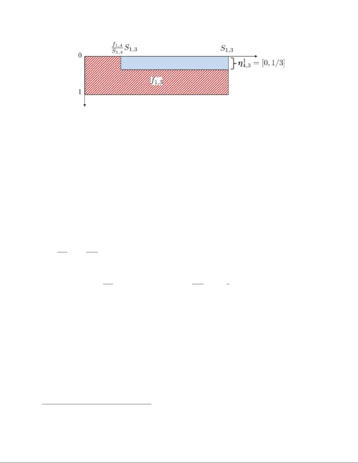
Macroscopic Mo deling, Calibration, and Sim ulation of Managed Lane-F reew a y Net w orks, P art I: T op ological and Phenomenological Mo deling Matthew A. W righ t, Rob erto Horo witz, Alex A. Kurzhanskiy Abstract T o help mitigate road congestion caused by the unrelen ting gro wth of traﬃc demand, many transit authorities ha ve implemen ted managed lane p olicies. Managed lanes typically run parallel to a freew ay’s standard, general-purp ose (GP) lanes, but are restricted to certain types of vehicles. It was originally though t that managed lanes would improv e the use of existing infrastructure through incen tivization of demand-managemen t b eha viors like carpo oling, but implementations ha ve often b een c haracterized by unpredicted phenomena that is often to detrimental system p erformance. Developmen t of traﬃc mo dels that can capture these sorts of b eha viors is a k ey step for helping managed lanes deliver on their promised gains. T ow ards this goal, this pap er presents several macroscopic traﬃc mo deling to ols w e hav e used for study of freewa ys equipp ed with managed lanes, or “managed lane-freewa y netw orks.” The prop osed framew ork is based on the widely-used ﬁrst-order kinematic wa ve theory . In this mo del, the GP and the managed lanes are modeled as parallel links connected b y nodes, where certain t yp e of traﬃc ma y switc h b et ween GP and managed lane links. T wo types of managed lane conﬁguration are considered: full-access, where vehicles can switc h b et ween the GP and the managed lanes anywhere; and sep ar ate d , where such switching is allow ed only at certain locations called gates . W e describ e macroscopic mo deling considerations for b oth t yp es of netw ork topologies. W e also describ e methods to incorp orate three phenomena into our mo del that are particular to managed lane-freewa y netw orks: the inertia eﬀe ct , the friction eﬀect , and the smo othing eﬀe ct . The inertia eﬀect reﬂects drivers’ inclination to sta y in their lane as long as p ossible and switch only if this w ould obviously impro ve their tra v el condition. The friction eﬀect reﬂects the empirically-observ ed driver fear of mo ving fast in a managed lane while traﬃc in the adjacent GP lanes mo ves slo wly due to congestion. Finally , the smo othing eﬀect describ es how managed lanes can incr e ase throughput at b ottlenec ks b y reducing lane changes. W e present simple modeling techniques for each of these phenomena that ﬁt within the general macroscopic theory for arbitrary link and junction mo dels. In this pap er’s sequel, we presen t model calibration methodologies and simulation results. Keyw ords : macroscopic ﬁrst order traﬃc mo del, ﬁrst order no de model, multi-commodity traﬃc, man- aged lanes, HOV lanes, dynamic traﬃc assignmen t, dynamic net work loading, inertia eﬀect, friction eﬀect, smo othing eﬀect 1 In tro duction T raﬃc demand in the dev elop ed and dev eloping w orlds shows no sign of decreasing, and the resulting congestion remains a costly source of ineﬃciency in the built en vironment. One study (Schrank et al., 2015) estimated that, in 2014, delays due to congestion cost driv ers 7 billion hours and $160B in the United States alone, leading to the burning of 3 billion extra gallons of fuel. The historical strategy for accommo dating more demand has been construction of additional infrastructure, but in recent years planners hav e also dev elop ed 1 strategies to improv e the p erformance of existing infrastructure, b oth through impro ved road operations and demand management , which seeks to lo wer the num ber of vehicles on the road (Kurzhanskiy and V araiy a, 2015). One such strategy that has b een widely adopted in the United States and other developed coun tries is the creation of so-called manage d lanes (Ob en b erger, 2004). Managed lanes are implemented on freewa ys b y restricting the use of one or more lanes to certain vehicles. As an example, high-o ccupancy-v ehicle (HO V) lanes are intended to incen tivize carp ooling, whic h reduces the total n umber of cars on the road as a demand managemen t outcome (Chang et al., 2008). In addition to demand management, managed lanes pro vide an opp ortunit y for improv ed road operations through real-time, resp onsive traﬃc con trol. F or example, tolled express lanes giv e driv ers the opportunity to pay a toll to driv e parallel to the general-purp ose lanes on a (presumably less-congested) express lane. T raﬃc management authorities here ha ve an opp ortunity to adjust the toll amoun t in response to the real-time state of traﬃc on the netw ork. The p oten tial for managed lanes as instrumen ts for reactive, real- time traﬃc op erations–in addition to their demand-managemen t purp ose–has made them p opular among transp ortation authorities (Kurzhanskiy and V araiya, 2015). Ho wev er, the traﬃc-operational eﬀects of managed lanes are not alw ays straigh tforward or as rehabilitativ e as exp ected, as their presence can create complex traﬃc dynamics. Even in a freew a y with simple geometry , the dynamics of traﬃc ﬂow are complex and not fully understo od, and adding managed lanes alongside the non-managed, general-purp ose (GP) lanes only exacerbates this. In eﬀect, adding a managed lane creates t wo parallel and distinct, but coupled, traﬃc ﬂo ws on the same physical structure. When used as in tended, managed lanes carry ﬂo ws with diﬀerent densit y-velocity characteristics and v ehicle-type (e.g., strictly HO V s) comp ositions than the freewa y . When vehicles mov e b et ween the tw o lane ﬂows, these t wo heterogeneous ﬂo ws mix, and complex phenomena that are unobserv ed in GP-only freewa ys can emerge (see, e.g., Menendez and Daganzo (2007); Daganzo and Cassidy (2008); Cassidy et al. (2010, 2015); Liu et al. (2011); Jang and Cassidy (2012); Thomson et al. (2012); P onnu and Coifman (2015, 2017); Fitzpatric k et al. (2017); Kim and P ark (2018), and others). Making b etter use of managed lanes requires an understanding of the macroscopic b eha vior they induce. One widely-used to ol for understanding macroscopic traﬃc ﬂow behavior is the macroscopic traﬃc ﬂo w mo del. A rich literature exists on macroscopic mo dels for ﬂows on long roads, and at junctions where those roads meet, but an extension to the parallel-ﬂows situation created by placing a managed lane in parallel with a freewa y (a “managed lane-freewa y netw ork”) is not straightforw ard. F or example, the GP/managed lane in terface has been observ ed to exhibit unique phenomena, suc h as e.g., 1) a “friction eﬀect” (Liu et al., 2011; Jang et al., 2012), where vehicles in a GP lane adjacent to the managed lane(s) mov e s lo wer than what w ould b e exp ected based solely on their density of cars (Liu et al., 2011; Fitzpatric k et al., 2017) (a common theory is that these GP lane vehicles mov e slo wly out of fear that vehicles may suddenly mo ve out of the managed lane in front of them), or 2) a “smo othing eﬀect” at b ottlenecks (Menendez and Daganzo, 2007; Cassidy et al., 2010; Jang and Cassidy, 2012) that leads to an incr e ase d ﬂo w in the GP lanes closest to the managed lane(s) by reducing lane changes (brieﬂy , few er vehicles b eing eligible for the fastest lane means that fewer vehicles will change lanes - and in the pro cess of c hanging lanes, slo w do wn surrounding traﬃc - to enter it. See, e.g., Zheng (2014) for more information on the eﬀects of lane changes on macroscopic ﬂo w characteristics). In the presen t pap er, we prop ose simple mo dels for these emergent phenomena that ﬁt within the classic macroscopic kinematic w a ve theory . T o the b est of our knowledge, we presen t the ﬁrst macroscopic mo deling tec hnique for the smo othing eﬀect, and the ﬁrst prop osed model of the friction eﬀect that considers junctions betw een the managed and GP lanes (w e will discuss the diﬀerences b et ween our prop osed friction eﬀect model and ones previously proposed in the literature be lo w). This pap er presen ts macroscopic ﬂow mo deling to ols w e hav e used for simulation of managed lane-freew ay net works. W e b egin in Section 2 with a discussion of relev ant mo deling to ols from the literature, and how w e mak e use of them. Section 3 describ es net work structures for the tw o common managed lane conﬁgurations: gated-access and full-access (ungated) lanes. Section 4 describ es simple models for the emergen t phenomena that are particular to managed lane-freew ay netw orks: the friction, smo othing, and inertia eﬀects. In Part I I of this paper series (W right et al., 2019), we put all of these pieces together, discuss how to calibrate the full mo del, and presen t mo deling case studies of tw o freewa ys with managed lanes in California. 2 2 Managed Lane Mo deling The mo deling techniques presented in this pap er are based on the ﬁrst-order “kinematic w av e” macroscopic traﬃc ﬂow model. These mo dels describ e aggregate traﬃc ﬂows as ﬂuids following a one-dimensional con- serv ation la w. W e brieﬂy introduce our notation here, but do not discuss the basics of this class of models. Detailed reviews are av ailable in many references. 2.1 Mo deling basics In this sim ulation framework, a road is divided into discrete cells, whic h we refer to as links . Links are drawn b et w een no des : a link b egins at one no de and ends at another. Man y links may b egin and end at eac h node. Eac h link l is c haracterized b y densit y n l , the num b er of cars in the link. In a ﬁrst-order mo del, the traﬃc ﬂo ws are fully prescrib ed by the density . F rom timestep t to t + 1 , link l ’s density up dates according to the equation n l ( t + 1) = n l ( t ) + 1 L l   M X i =1 f il ( t ) − N X j =1 f lj ( t )   , (2.1) where L l is the length of link l , f il ( t ) is the ﬂow (num b er of v ehicles) lea ving link i and en tering link l at time t , f lj ( t ) is the ﬂow lea ving link l and en tering link j at time t , M is the n umber of links that end at link l ’s b eginning no de, and N is the n umber of links that begin at link l ’s ending no de. Computing the in ter-link ﬂows requires the use of t wo intermediate quan tities for each link. These are the link demand S l ( t ) , whic h is the n umber of vehicles that wish to exit link l at timestep t ; and the link supply , R l ( t ) , which is the n umber of v ehicles link l can accept at time t . Both S l and R l are functions of the density n l . The model that computes S l and R l from n l is often called the “fundamental diagram” or “link mo del,” and the mo del that computes the ﬂo ws from all links’ supplies and demands is often called the “no de model.” A brief outline of how ﬁrst-order macroscopic simulation of a road net work (sometimes called a dynamic network lo ading simulation) is p erformed could be: 1. A t time t , use the link mo del for eac h link l to compute the link’s demand S l ( t ) and supply R l ( t ) as a function of its density n l ( t ) . 2. Use the no de mo del for each no de to compute the inter-link ﬂows f ij for all incoming links i and outgoing links j as functions of S i ( t ) , R j ( t ) , and information ab out v ehicles’ desired mov ements ij . 3. Up date the state of eac h link using (2.1). 4. Incremen t t and rep eat until the desired sim ulation end time is reac hed. The to ols describ ed in this pap er are compatible with any such link mo del. W e make use of a particular no de mo del that we hav e studied in W right et al. (2016, 2017). An aspect of this node mo del of particular relev ance to managed lane mo deling is our “relaxed ﬁrst-in-ﬁrst-out (FIF O) rule” construction (W righ t et al., 2017). This is necessary for mo deling the ﬂows b etw een the GP and managed lanes. Without a FIFO relaxation, congestion in one of the t wo lane groups could blo c k traﬃc in the other when that ma y be unrealistic (see W right et al. (2017, Section 2.2) for a detailed discussion). So far, we hav e presen ted ingredients for a mo del that, while able to express many simple net work topologies b y joining links and no des, do es not capture several imp ortan t behaviors in managed lane-freew ay netw orks. The next three Sections brieﬂy ov erview the additions to the standard mo del that will b e explained in greater detail in the remainder of the pap er. 3 2.2 Multiple classes of vehicles and driv ers In (2.1), w e describ e the num b er of v ehicles in a link as a single n umber, n l . In this form ulation, all vehicles are treated the same. How ever, for simulation in a managed lane-freew ay netw ork, it mak es sense to break n l in to diﬀerent classes of v ehicles and/or drivers. F or example, for a freew ay with an HO V lane facility , we migh t consider tw o classes: HOV s and non-HO V s. T o this end, (2.1) can be rewritten as n c l ( t + 1) = n c l ( t ) + 1 L l   M X i =1 f c il ( t ) − N X j =1 f c lj ( t )   , (2.2) where c ∈ { 1 , . . . , C } indexes v ehicle classes (often called “commo dities” in the traﬃc literature). Extending the densit y up date equation to multiple classes means that the link and node mo dels must also b e extended to pro duce p er-class ﬂows f c ij . In this pap er, we will not specify a particular link mo del, but assume use of one that pro duces p er-class demands S c i and ov erall supplies R j (the no de mo del, in computing the f c ij , is resp onsible for splitting the av ailable supply R j among the diﬀerent demanding v ehicle classes). Examples of this t yp e of link mo del include those considered in W ong and W ong (2002), Daganzo (2002), and v an Lint et al. (2008) (examples of multi-class link mo dels of second- or higher-order include those of Ho ogendoorn and Bo vy (2000). These types of mo dels hav e higher-order analogs of supply and demand). 2.3 T oplogical expression of managed lane-freewa y net works In b oth (2.1) and (2.2), w e describ e a link in terms of its total density n l and its breakdown into p er- commo dit y p ortions, n c l . By discretizing the road in to these one-dimensional links, we lose information ab out diﬀerences b et ween v ehicle prop ortions across lanes, as well as inter-lane and lane-changing behavior. This b ecomes a problem if suc h unmo deled behavior is of in terest. In our setting, this means that mo deling a freewa y with a managed lane should not be d one with a single link following (2.1) or (2.2), as it would b e imp ossible to study the managed lane-freewa y netw ork b ehavior of interest. Mo deling diﬀerences in v ehicle density across lanes is natural in microscopic and mesoscopic (see, for example, T reib er et al. (1999); Ho ogendoorn and Bo vy (1999); Ngoduy (2006), and others) models, but macroscopic mo dels, in their simplicit y , hav e less readily-accessible av enues for including these diﬀerences. One straight- forw ard metho d is to mo del eac h lane as a separate link, as in, e.g. Bliemer (2007) or Shiomi et al. (2015). Ho wev er, this metho d has a few drawbac ks. First, it requires the addition of some lane-assignment metho d to prescrib e the prop ortions of eac h vehicle class c for each lane (such as a logit mo del as used in F arhi et al. (2013) and Shiomi et al. (2015)), which requires not-alw ays-accessible data for calibration. Second, drastically increasing the num b er of links in a macroscopic mo del will necessarily increase the size of the state space and mo del complexity , which is, in a sense, incompatible with the ov erall goal of selecting a macroscopic mo del o ver a micro- or mesoscopic model: some of the “macro” in the macroscopic mo del is lost. Instead, in this paper we choose to mo del the GP lanes (or “GP lane group”) as one link and the parallel managed lanes (or “managed lane group”) as another link. Applied to an en tire length of road, this creates a net work topology of tw o “parallel c hains” of links - one GP and one managed. The tw o chains will share no des, but cross-ﬂo ws b et ween the chains are p ermitted only in lo cations where there is physical access (i.e., no physical barriers) and p olicy access (i.e., no double solid line s under U.S. traﬃc markings). Where cross-ﬂo ws are possible, we do not use a logit mo del, but instead a driv er b eha vior model ﬁrst in tro duced in W righ t et al. (2017). This t wo-c hain model is similar to the one described in Liu et al. (2012), though in this reference, GP-managed lane crossﬂows were not considered. 4 2.4 Mo deling emergen t phenomena particular to managed lane-freew a y net- w orks Our techniques for mo deling the friction, smo othing, and inertia eﬀects are ro oted in a full-picture view of the macroscopic modeling framew ork. As we will see, w e propose isolating eac h of these “eﬀects” to one comp onen t of the traditional macroscopic mo deling framew ork: the friction eﬀect mo del is based on a principled feedbac k mec hanism of the fundamental diagram, the inertia eﬀect mo del is included in modeling of driver choices for which of the t wo lane groups they will take, and the smo othing eﬀect mo del emerges from a particular recently-dev elop ed no de mo del construction. 3 F ull- and Gated-A ccess Managed Lane-F reew a y Net w ork T op ologies W e will consider tw o types of managed lane-freewa y netw ork conﬁgurations: ful l ac c ess and sep ar ate d with gate d ac c ess . In a a full-access conﬁguration, the managed lane(s) are not physically separated from the GP lane(s), and eligible vehicles may switc h b et ween the tw o lane groups at any location. Often, full-access managed lane(s) are sp ecial-use only during certain perio ds of the day , and at other times they serve as GP lane(s) (e.g., HOV lanes are often accessible to non-HO V s outside of rush hour). On the other hand, in a gated-access conﬁguration, traﬃc ma y switc h b et ween the managed lane(s) and GP lane(s) only at certain lo cations, called gates ; at non-gate lo cations, the tw o lane groups are separated by road markings (i.e., a double solid line in the U.S.) or a physical barrier. Usually , gated-access managed lanes are sp ecial-use at all times. The implemented managed lane access sc heme dep ends on jurisdiction. F or example, full-access lanes are common in Northern California, and separated lanes are common in Southern California. The diﬀerences in physical geometry and access p oin ts b et ween the t wo access t yp es requires t wo diﬀeren t t yp es of topology in constructing a net work for a macroscopic mo del. 3.1 Note on link and no de mo dels used in this section As discussed in the previous Section, w e attempt to b e agnostic with regards to the particular link mo del (e.g., ﬁrst-order fundamen tal diagram) used in our implemen tations. Ho w ever, in our model of the friction eﬀect in Section 4.1, w e parameterize friction b eing in eﬀect on a particular link l for a particular vehicle class c at time t by adjusting that link’s demand S l ( t ) . F or that discussion only , w e sp ecify a particular link mo del. This link model is reviewed in App endix A. The no de model used here and for the remainder of this pap er, when a particular form is necessary , is the one discussed in W right et al. (2016, 2017). W e use this no de mo del b ecause it handles m ulti-commo dit y traﬃc, optimizes the utilization of do wnstream supply , mak es use of input link priorities and has a relaxation of the “conserv ation of turning ratios” or “ﬁrst-in-ﬁrst-out” (FIFO) constraint of most no de mo dels. This last feature allows us to describe a set of GP lanes just upstream of an oﬀramp with one link, and handle a condition of a congested oﬀramp b y having the congestion spill back on to only the oﬀramp-serving lanes of the GP link (as opp osed to the entiret y of the GP link). See W right et al. (2017, Section 3) and W righ t et al. (2016) for more discussion. 3.2 F ull-access managed lanes A full-access managed lane conﬁguration is presen ted in Figure 1: GP and managed links (recall, as discussed ab o v e, all GP lanes and all managed lanes are collapsed in to one link eac h) are parallel with the same geometry 5 Figure 1: F reewa y with full-access managed lane. ML = Managed Lane. and share the same beginning and ending node pairs; traﬃc ﬂo w exchange b et ween GP and managed lanes can happ en at every node. Note that in Figure 1, we use a slightly irregular n umbering scheme so that it is clear whether a link is a GP link, managed lane link, or ramp link. Parallel links in the graph hav e n umbers made up of the digit of their terminating no de, with GP links having one digit (i.e., link 1), managed lane links having tw o (i.e., link 11), and ramp links having three (i.e., link 111). Note also that w e use a U.S.-st yle, driving-on-the-righ t conv ention here, with the managed lane(s) on the left of the GP lanes and the ramps on the far right. Links that are to o long for mo deling purposes (i.e., that create to o lo w-resolution a mo del) may b e brok en up into smaller ones b y creating more n odes, suc h as nodes 2 and 3 in Figure 1. F undamental diagrams for parallel GP and managed lane links may be diﬀeren t (Liu et al., 2011). W e introduce tw o vehicle classes ( C = 2 ): c = 1 corresponds to the GP-only traﬃc and c = 2 corresponds to the special traﬃc. When the managed lane(s) is (are) active, c = 1 -traﬃc is conﬁned to the GP link, whereas c = 2 -traﬃc can use b oth the GP and managed lane links. W e denote the p ortion of v ehicles of class c in link i that will attempt to enter link j as β c i,j . This quan tity is called the split ratio. 3.2.1 Split ratios for full-access managed lanes W e mak e an assumption that b oth vehicle classes take oﬀramps at the same rate. F or example, for node 1 in Figure 1, w e migh t say that β 1 i, 222 = β 2 i, 222 , β i, 222 . Strictly sp eaking, it is not necessary to assume that the β c i, 222 are equal for all c . How ever, in practice the oﬀramp split ratios are typically estimated from ﬂow coun t data tak en from detectors on the oﬀramp and freew ay . Generally speaking, these detectors cannot iden tify v ehicle type, so the only quan tity estimable is a ﬂow-w eighted av erage of the quantities β c i, 222 . T o estimate the class-speciﬁc split ratios, one needs some extra kno wledge of the tendency of eac h class to take each oﬀramp (for example, that GP-only vehicles are half as likely as sp ecial traﬃc to tak e a certain oﬀramp). Assuming that each class exits the freew ay at the same rate is a simple and reasonable-seeming assumption. This same problem of uniden tiﬁability from typical data app ears in sev eral other split ratios. First, it may not b e p ossible to tell how many v ehicles taking an oﬀramp link come from the upstream GP , managed lane, or (if presen t) onramp link. In this case, some assumptions m ust then b e made. F or example, three diﬀeren t assumptions that ma y b e reasonable are (1) that v ehicles in each link i tak e the oﬀramp at the same rate; or (2) that no vehicles from the managed lane(s) are able to cross the GP lanes to take the oﬀramp at this no de, and that no v ehicles entering via the onramp, if one is presen t, exit via the oﬀramp at the same no de; or (3) that vehicles in GP and managed links take the oﬀramp at the same rate, while no vehicles coming from the onramp are directed to the oﬀramp. Lo oking bac k at no de 1 in Figure 1 again, assumption (1) w ould say the β i, 222 are equal for all i ; assumption (2) w ould say β 11 , 222 = β 111 , 222 = 0 ; and assumption (3) w ould say β 1 , 222 = β 11 , 222 and β 111 , 222 = 0 . The b est assumption for each no de will depend on the road geometry for that particular part of the road (how near the oﬀramp is to an y onramps, how many GP lanes a vehicle in a managed lane would hav e to cross, etc.). Second, the crossﬂows b etw een the GP and managed lane links are not observ able. Even if there exist detectors immediately upstream and do wnstream of the node where traﬃc can switch b et w een GP and 6 managed lanes, it is impossible to uniquely identify the crossﬂows. In a sim ulation, these crossﬂo ws m ust be go verned by some driver c hoice mo del. Putting together these assumptions and the sp ecial-traﬃc-only p olicy for the managed lane, w e can summa- rize most of the necessary split ratios needed for computing ﬂows in a no de model. F or example, for no de 1 in Figure 1, β 1 i,j =        j = 2 j = 22 j = 222 i = 1 1 − β 1 , 222 0 β 1 , 222 i = 11 n/a n/a n/a i = 111 1 − β 111 , 222 0 β 111 , 222 β 2 i,j =        j = 2 j = 22 j = 222 i = 1 − − β 1 , 222 i = 11 − − β 11 , 222 i = 111 − − β 111 , 222 where “n/a” means that the split ratios β 1 11 ,j are not applicable, as there should b e no vehicles of class c = 1 in the managed lane. The split ratios marked with a dash are those ab ov e-mentioned ﬂo ws that are unobserv able and come from some driver c hoice model. Of course, whatever method is chosen to compute these unknown split ratios, w e must hav e β 2 i, 2 + β 2 i, 22 = 1 − β 2 i, 222 . Similarly , for no de 2, which do es not hav e an onramp or an oﬀramp, β 1 i,j =    j = 3 j = 33 i = 2 1 0 i = 22 n/a n/a β 2 i,j =    j = 3 j = 33 i = 2 − − i = 22 − − with “n/a” and the dash meaning the same as abov e. As previously mentioned, full-access managed lanes often ha ve certain time perio ds during which nonsp ecial ( c = 1 ) traﬃc is allow ed in to the managed lane. W e can mo del this change in p olicy simply by c hanging the split ratios at the no des. F or no de 1, for example, the nonrestrictiv e policy is enco ded as β c i,j =        j = 2 j = 22 j = 222 i = 1 − − β 1 , 222 i = 11 − − β 11 , 222 i = 111 − − β 111 , 222 for c = { 1 , 2 } , and for node 2 as β c i,j =    j = 3 j = 33 i = 2 − − i = 22 − − for c = { 1 , 2 } . In other words, the managed lane link is treated as additional GP lane(s), and the split ratios go verning the crossﬂo ws betw een the t wo links should be found from the driv er c hoice mo del for both v ehicle classes. 3.2.2 No de mo del for full-access managed lane-freew ay net works As mentioned in Section 3.1, w e make use of the no de mo del discussed in W right et al. (2016, 2017) to describ e a freewa y netw ork with managed lanes. This node model diﬀerentiates itself from others in that 7 it deals with multi-commodity traﬃc ﬂow, optimally utilizes the av ailable supply , mak es use of input link priorities, and has a relaxation of the common FIFO constraint. By default, link priorities can b e taken prop ortional to link capacities. T o explain relaxed FIFO, sa y that some link i has vehicles that wish to en ter b oth links j and j 0 . If link j 0 is jammed and cannot accept any more v ehicles, a strict FIF O constraint w ould sa y that the v ehicles in i that wish to en ter j 0 will queue at i ’s exit, and block the v ehicles that wish to en ter j . In a m ulti-lane road, how ever, only certain lanes may queue, and traﬃc to j may still pass through other lanes. The relaxation is encoded in so-called “mutual restriction in terv als” η i j 0 j ⊆ [0 , 1] . This in terv al partly describ es the o verlapping regions of link i ’s exit that serve both links j and j 0 . F or η i j 0 j = [ y , z ] , a z − y p ortion of i ’s lanes that serv e j also serve j 0 , and will b e block ed by the cars queueing to enter j 0 when j 0 is congested. F or example, if j is served by three lanes of i , and of those three lanes, the leftmost also serv es j 0 , we w ould ha ve η i j 0 j = [0 , 1 / 3 ] . As an example, we consider again node 1 in Figure 1. Say that the GP links (1 and 2) hav e four lanes, that the managed lane links (11 and 22) ha ve t wo lanes, and that the onramp merges into and the oﬀramp div erges from the righ tmost GP lane. F urther, we say that when the managed lane link is congested, v ehicles in the GP lanes that wish to enter the managed lanes will queue only in the leftmost GP lane. On the other hand, when the GP link is congested, vehicles in the managed lanes that wish to enter the GP lanes will queue only in the righ tmost managed lane. Finally , we supp ose that jammed oﬀramp (222) will cause v ehicles to queue only in the righ tmost GP lane. T aking together all of these statements, our m utual restriction in terv als for this example are: η 1 j 0 j =        j = 2 j = 22 j = 222 j 0 = 2 [0 , 1] [0 , 1] [0 , 1] j 0 = 22 [0 , 1 / 4 ] [0 , 1] ∅ j 0 = 222 [ 3 / 4 , 1] ∅ [0 , 1] η 11 j 0 j =        j = 2 j = 22 j = 222 j 0 = 2 [0 , 1] [0 , 1 / 2 ] ∅ j 0 = 22 [0 , 1] [0 , 1] ∅ j 0 = 222 ∅ ∅ [0 , 1] η 111 j 0 j =        j = 2 j = 22 j = 222 j 0 = 2 [0 , 1] [0 , 1] [0 , 1] j 0 = 22 ∅ [0 , 1] ∅ j 0 = 222 [0 , 1] [0 , 1] [0 , 1] . T o read the ab o v e tables, recall that as written, j 0 is the congested, restricting link, and j is the restricted link. These chosen restriction in terv als allow for expected b eha vior in this netw ork, such as a congested GP link causing p ossible queueing in the right managed lane (if some drivers are trying to en ter the GP link), but no spillbac k into the left managed lane. 1 F or a detailed discussion on how mutual restriction in terv als are included in the node mo del’s ﬂow calculations and solution algorithms, see W right et al. (2016, 2017). 3.3 Separated managed lanes with gated access A separated, gated-access managed lane conﬁguration is presen ted in Figure 2. Unlik e the full-access con- ﬁguration, the GP and managed lane link c hains do not necessarily meet at every no de. Instead, they need only meet at a few lo cations, where vehicles can mov e into and out of the managed lane(s). Note that, unlik e the full-access conﬁguration, there is no need for GP and managed lane links to b e aligned. As labeled in Figure 2, the no des where the tw o link c hains meet are called gates (as an aside, one w ay to describ e the full-access managed lane conﬁguration would b e that ev ery node is a gate). Similar to our 1 In this example, we assume that the managed lane has t wo sublanes — left and right. 8 construction of excluding GP-only traﬃc from the managed lane in the full-access case, w e can disable ﬂow exc hange at a given gate b y ﬁxing split ratios so that they k eep traﬃc in their lanes. F or example, to disable the gate (the ﬂow exchange b etw een the tw o lanes) at no de 2 in Figure 1, we set β c 2 , 3 = 1 and β c 22 , 33 = 1 (this means that β c 2 , 33 = 0 and β c 22 , 3 = 0 ), c = 1 , 2 . Thus, the full-access managed lane can be easily con verted into the separated managed lane by setting non-exchanging split ratios ev erywhere but designated gate-no des. In practice, a gate is stretch of freewa y that may b e a few h undreds of meters long (Cassidy et al., 2015), and, p oten tially , we can designate t wo or three sequen tial no des as gates. In this paper, ho wev er, we mo del a gate as a single node. Figure 2: F reewa y with separated managed lane and gates. ML = Managed Lane. F or the gated-access conﬁguration, w e suggest setting mutual restriction coeﬃcients in the same manner as full-access managed lanes, in Section 3.2.2. Compared to the full-access managed lane conﬁguration, the gated-access conﬁguration has a smaller friction eﬀect (Jang et al., 2012): drivers in the separated managed lane feel somewhat protected by the buﬀer, whether it is virtual (double solid line) or real (concrete), from vehicles c hanging abruptly from the slow mo ving GP lane and, therefore, do not drop sp eed as dramatically . The degree to which the friction eﬀect is mitigated is disputed (e.g., see F o otnote 3 in Cassidy et al. (2015)), but ov erall the b ottlenec ks created by the gates are m uch greater instigators of congestion (Cassidy et al., 2015). Inclusion of the friction eﬀect in mo deling separated managed lane conﬁgurations is th us not as essential as in modeling the full-access case. By similar logic, the smoothing eﬀect should b e exp ected to be less prominent. If a physical barrier prev ents lane c hanging in to the managed lane, then there will be no lane c hanging into the managed lane - the ﬂo w is already as “smo othed” as p ossible. It will become apparent in section 4.3, when w e discuss our smo othing eﬀect model, that in our mo del the degree of traﬃc smoothing is indeed maximized when the inter-link split ratios are zero (as they are in the non-gate no des). 3.3.1 Mo deling a ﬂo w of v ehicles from the managed lanes to the oﬀramps Recall from Section 3.2.1 that, in the full-access managed lane model, we can mo del vehicles mo ving from the managed lane link to oﬀramps in a straigh tforward manner, by setting corresp onding split ratios (for example, β c 11 , 222 , c = 1 , 2 , for no de 1 in conﬁguration from Figure 1). F or the gated-access conﬁguration, ho wev er, mo deling traﬃc as moving from the managed lanes to oﬀramps is more complicated: generally , gates do not coincide with oﬀramp lo cations. In fact, there are typically b et ween tw o and ﬁv e oﬀramps b et w een tw o gate lo cations. These oﬀramps cannot b e accessed directly from the managed lane. T o mo del a v ehicle ﬂow that originates at the managed lane link, go es through a gate to the GP lane link, and then tak es the correct oﬀramp (and doing so at some rate that matc hes external origin-destination data), requires a more in volv ed modeling and b ookkeeping construction. T o resolve this c hallenge, our gated-access model introduces new vehicle classes in addition to the c = 1 (GP-only) and c = 2 (sp ecial) traﬃc used in the full-access mo del of Section 3.2. These additional classes will b e used to distinguish subsets of the sp ecial traﬃc p opulation by its destination oﬀramp. If K is the largest num b er of oﬀramps betw een t w o adjacen t gates, then altogether w e hav e C = K + 2 v ehicle classes: c = 1 , 2 , e 1 , . . . , e K , where e k indicates the class of v ehicles that will exit through the k -th oﬀramp after 9 lea ving the managed lane through the gate. By deﬁnition, traﬃc of type c = e k may exist in the GP lane segmen t b et ween gate 1 and oﬀramp e k , but there is no tr aﬃc of this typ e either in the GP link segmen t b et w een oﬀramp e k and gate 2 or in the managed lane link. This mov ement pattern is ensured b y setting c onstant split ratios: β e k i x 1 = 1 , i = 1 , 11 , 111 , direct all e k -t yp e traﬃc to the GP link at gate 1 ; β e k x k e k = 1 , direct all e k -t yp e traﬃc to oﬀramp e k ; β e k x k 0 e k 0 = 0 , k 0 6 = k , do not send any e k -t yp e traﬃc to other oﬀramps , (3.1) where k = 1 , . . . , K , and x k denotes the input GP link for the no de that has the output link e k (see Figure 2). V ehicles of class c = e k do not en ter the netw ork via onramps or the upstream boundary , but instead are conv erted from sp ecial c = 2 traﬃc as it leav es the managed lane(s) through the gate. W e p erform this con version as part of the link mo del computation, suc h that the total demand for the switching link, P C c =1 S c l remains the same before and after the switc h. The exact link on whic h this switc hing takes place is the managed lane link immediately upstream of the gate (e.g., link 11 in Figure 2). W e say that the amount of traﬃc that should change from vehicle class c = 2 to vehicle class e k at time t is (using link 11 as an example) n 2 11 ( t ) β 2 x k e k ( t ) v 11 ( t ) , where v 11 ( t ) is in units of v ehicles p er simulation timestep (this factor is included so that the switching done is prop ortional to link 11’s outﬂo w, rather than its density), and β 2 x k e k ( t ) is the split ratio from x k , the GP link immediately upstream of exit e k , and the exit e k at time t . This statement is based on the assumption that the v ehicles in the managed lane link will exit the freew ay through exit e k at the same rate as special ( c = 2 ) vehicles that happ ened to sta y in the GP lanes. That is, if a β 2 x k e k p ortion of c = 2 vehicles intend to lea ve the GP lanes through exit e k , then a β 2 x k e k p ortion of the c = 2 vehicles in the managed lane(s) will lea ve the managed lane link at the closest upstream gate and leav e the net work at exit e k when they reach it. Note that if there are K 0 < K oﬀramps b et ween t wo particular gates, then no v ehicles should switch to type c = e k , k ∈ { K 0 + 1 , . . . , K } at the upstream gate, as they would ha ve no ramp to exit through. W e now explain how e k -t yp e traﬃc appears in the system. The original d emand d c l ( · ) is speciﬁed at origin links l for commo dities c = 1 , 2 , and d e k l ( · ) ≡ 0 , k = 1 , . . . , K . Destination sp eciﬁc traﬃc app ears in the managed lane links that end at gate-no des b y assigning destinations to p ortions of the type-1 (GP-only) and t yp e-2 (managed lane-eligible) traﬃc in those links. W e prop ose using oﬀramp split ratios β c x k ,e k , c = 1 , 2 , k = 1 , . . . , K , to determine p ortions of managed lane traﬃc to b e assigned particular destinations. The destination assignmen t algorithm at a given time t , for a given HOV link ending with a gate-no de, is describ ed next. Without loss of generality , we will refer to Figure 2 and managed lane link 11 ending at the gate-no de 1 in this description. Using Figure 2 as a reference, we can no w formally describ e the pro cedure for destination assignmen t to traﬃc in the managed lane link. 1. Giv en are v ehicle coun ts per commo dit y n c 11 , c = 1 , 2 , e 1 , . . . , e K ; free ﬂow sp eed v 11 ; and oﬀramp split ratios β 1 x k ,e k and β 2 x k ,e k , k = 1 , . . . , K . 2 2. Initialize: ˜ n c 11 (0) := n c 11 , c = 1 , 2 , e 1 , . . . e K ; k := 1 . 3. Assign e k -t yp e traﬃc: ˜ n e k 11 ( k ) = ˜ n e k 11 ( k − 1) + β 1 x k ,e k v 11 ˜ n 1 11 ( k − 1) + β 2 x k ,e k v 11 ˜ n 2 11 ( k − 1); (3.2) ˜ n 1 11 ( k ) = ˜ n 1 11 ( k − 1) − β 1 x k ,e k v 11 ˜ n 1 11 ( k − 1); (3.3) ˜ n 2 11 ( k ) = ˜ n 2 11 ( k − 1) − β 2 x k ,e k v 11 ˜ n 2 11 ( k − 1) . (3.4) 2 If a given GP segment connecting t wo adjacent gates has K 0 oﬀramps, where K 0 < K , then assume β 1 x k ,e k = β 2 x k ,e k = 0 for k ∈ ( K 0 , K ] . 10 4. If k < K , then set k := k + 1 and return to step 3. 5. Up date the state: n c 11 = ˜ n c 11 ( K ) , c = 1 , 2 , e 1 , . . . , e K . After the switches to c = e k class traﬃc hav e b een done, there may b e unresolved split ratios for b oth classes c = 1 and c = 2 at the gates (similar to the dashed split ratios in the tables in Section 3.2.1). These split ratios should b e ﬁlled in with the same to ols as those in Section 3.2.1: some sort of driv er lane c hoice b eha vior. 4 Mo deling Emergen t Phenomena P articular to Managed Lane- F reew a y Net works As previously discussed, managed lane-freewa y net works exhibit macroscopic phenomena that do not arise in situations where the managed lanes may act as traditional GP lanes 3 . These unique behaviors are caused by the interactions b et ween the qualitativ ely diﬀeren t the ﬂows in the GP lanes and the neigh b oring managed lanes. In this section, we describ e simple physical mo dels for three suc h b eha viors: the friction eﬀect, the smo othing eﬀect, and the inertia eﬀect. 4.1 F riction eﬀect The friction eﬀe ct is an empirically-observed phenomenon in situations where managed lanes are relatively uncongested, but the managed-lane traﬃc will still slo w down when the adjacent GP lanes congest and slow do wn (see Daganzo and Cassidy (2008); Liu et al. (2011); Thomson et al. (2012); Fitzpatric k et al. (2017), etc.). It has b een hypothesized (Jang and Cassidy, 2012) that this phenomenon arises from the managed-lane driv ers’ fear that slow er-mo ving vehicles will suddenly and dangerously change into the managed lane ahead of them. W e suggest modeling the friction eﬀect based on a fe e db ack me chanism that uses the diﬀerence of sp eeds in the parallel GP and managed lane links to scale do wn the ﬂo w (and therefore the sp eed) out of the managed lane link if necessary . T o explain the concept, w e again refer to Figure 1 and consider parallel links 1 (GP) and 11 (managed lane). Recall that, under a ﬁrst-order model (2.2), the sp eed of traﬃc in link l at time t is v l ( t ) = ( P C c =1 P N j =1 f c lj ( t ) P c =1 n c l ( t ) if P c c =1 n c l ( t ) > 0 , v f l ( t ) otherwise , (4.1) where v f l ( t ) is the theoretical free ﬂo w sp eed of link l at time t . W e sa y that the friction eﬀect is present in managed lane link 11 (following the notation of Figure 1) at time t if v 1 ( t − 1) < min n v f 1 , v 11 ( t − 1) o , (4.2) 3 One of these eﬀects, the smoothing eﬀect, was even observed in a previous study (Cassidy et al., 2010) to be present in a managed lane-freew ay network, but not present on the same se ction of r o ad in another perio d of the day when the managed lane p olicy w as not enforced (in that particular case, carp ool/HOV lane enforcemen t during the peak hours) 11 whic h means that (1) the GP link is in congestion (its sp eed is b elo w its current free ﬂow speed), and (2) the speed in the GP link is less than the sp eed in the managed lane link. W e denote this sp eed diﬀeren tial as: ∆ 11 ( t ) = v f 11 − v 1 ( t − 1) . (4.3) It has b een observed (Jang et al., 2012) that the magnitude of the friction eﬀect — the degree to which managed-lane drivers slow down tow ards the GP lane’s traﬃc speed — depends on the physical conﬁguration of the road. F or example, less of a friction eﬀect will b e presen t on managed lanes that are separated from the GP lanes by a buﬀer zone than those that are con tiguous with the GP lanes (Thomson et al., 2012; Jang et al., 2012; Fitzpatrick et al., 2017), and the presence of a concrete barrier w ould practically eliminate the friction eﬀect. Other factors that ma y aﬀect this magnitude include, for example, whether there is more than one managed lane, or whether there is a shoulder lane to the left of the managed lane that drivers could sw erve into if necessary . T o enco de this v ariability in the magnitude of the friction eﬀect in managed lane link 11, w e introduce σ 11 ∈ [0 , 1] the friction c o eﬃcient of this link. The friction co eﬃcient reﬂects the strength of the friction. Its v alue depends on the particular managed conﬁguration and is c hosen b y the mo deler. A v alue of σ 11 = 0 means there is no friction (which ma y b e appropriate if, perhaps, the managed lane(s) are separated from the GP lanes by a concrete barrier), and σ 11 = 1 means that the managed lane link sp eed tracks the GP link sp eed exactly . When the friction eﬀect is activ e (i.e., when (4.2) is true), we adjust the fundamen tal diagram of the managed lane link b y scaling down its theoretical free ﬂow sp eed v f l ( t ) , and propagate that c hange through the rest of the fundamental diagram parameters. The exact mathematical c hanges will of course b e diﬀeren t for every diﬀeren t form of fundamental diagram. F or the particular fundamen tal diagram discussed in Appendix A, this means adjusting the free ﬂo w sp eed and capacit y as follo ws: ˆ v 11 ( t ) = v f 11 ( t ) − σ 11 ∆ 11 ( t ); (4.4) ˆ F 11 ( t ) = ˆ v 11 ( t ) n + 11 , (4.5) where n + 11 is the high critical densit y (see Appendix A for its deﬁnition), and using these adjusted v alues in the calculation of the sending function (A.1), S c 11 ( t ) = ˆ v 11 ( t ) n c 11 ( t ) min ( 1 , ˆ F 11 ( t ) ˆ v 11 ( t ) P C c =1 n c 11 ( t ) ) . (4.6) F or the fundamental diagram of App endix A, w e must also chec k whether C X c =1 n c 11 ( t ) < ˆ F 11 ( t ) v f 11 − ∆ 11 ( t ) = ˆ v 11 ( t ) n + 11 ( t ) v f 11 − ∆ 11 ( t ) . (4.7) If not, then applying friction will lead to the managed lane link speed falling b elo w the GP link sp eed, and the unadjusted sending function should b e used (the p ossibilit y of this happ ening is due to the use of t wo critical densities to create App endix A’s fundamen tal diagram’s “bac kwards lam b da” shape). Again, the exact form of (4.6), the sending function with friction, will dep end on the link’s original funda- men tal diagram mo del. 4.1.1 Comparison with related work W e are not the ﬁrst to prop osed mo deling the friction eﬀect by adjusting the fundamen tal diagram of the managed lane as a function of the state of the GP lane(s). In particular, Liu et al. (2012) consider a stretch 12 of an HOV-equipped freew ay where the tw o classes of lanes are separated by a buﬀer, and prop ose to ﬁt t wo diﬀeren t sets of ﬂow parameters for the HOV lane based on whether or not the GP lanes are congested. Our metho d diﬀers in formulation and p oten tial uses. First, we prop ose a principled mo diﬁcation to the fundamen tal diagram that is based on observ ations of how the friction eﬀect actually aﬀects the managed lane’s fundamen tal diagram, via the idea of low ering the theoretical managed lane free-ﬂow sp eed. Examining (4.4) again, this formulation has an eﬀect on the fundamen tal diagram’s free-ﬂow speed that is linear in the sp eed diﬀeren tial. This formulation w as chosen based on prior studies: evidence of a friction eﬀect reducing managed lane sp eed in a form that is linear in the sp eed diﬀerential was rep orted in, e.g., Jang et al. (2012). This is in contrast to earlier mo dels that switc h b et ween tw o distinct and discrete sets of fundamen tal diagram parameters based on a GP congestion threshold (i.e., a piecewise rather than linear relationship). Our theoretically-based fundamental diagram adjustmen t is also motiv ated by the common use for macro- scopic simulation as a forecasting to ol. T raﬃc simulation to ols are often used to study p oten tial eﬀects of prop osed, but not y et dev elop ed, infrastructure construction (Kurzhanskiy and V araiya, 2015). Moreov er, the particular infrastructure inv estment of managed lane construction in tro duces the p oten tial for additional p olicy choices (e.g., whether to restrict an HOV lane to vehicles with at least 2 o ccupan ts or those with at least 3 o ccupan ts, the tolling prices in a tolled express lane, etc.), eac h with their o wn feedback eﬀects of the ﬂo w on the road, and underlying demand managemen t. These complexities hav e motiv ated the dev elopment of new simulation to ols sp eciﬁcally for new managed lane t yp es (Guoh ui et al., 2009). In the business and p olicy worlds, these complex inv estments with many feedback eﬀects are ev aluated through Monte Carlo sim ulation of principled models (Kurzhanskiy and V araiya, 2015). Our friction eﬀect mo del is motiv ated in part by this type of use case, where a theoretically-justiﬁed mo del is to b e used in situations where data is unav ailable due to the construction having not o ccurred yet. On the other hand, of course, if a traﬃc engineer is studying an already-existing managed lane-freewa y netw ork, where data measuring the friction eﬀect can be collected, it makes sense to ﬁt a friction eﬀect mo del based on those data. 4.2 Inertia eﬀect A t the end of Section 3.3.1, we men tioned that some split ratios will lik ely be undeﬁned after switc hing c = 2 class v ehicles to the c = e k classes. In particular, c = 2 class v ehicles in the upstream GP link (e.g., link 1 in Figure 2) and remaining c = 2 vehicles in the upstream managed lane link (e.g. link 11 in Figure 2) will need to decide whether to pass through the gate or remain in their curren t lane. Sample to ols for modeling driv er lane choices such as these include the class of “logit” logistic regression mo dels (McF adden, 1973), or dynamic split ratio solvers suc h as the one presen ted in W right et al. (2018). When applied to lane choice (e.g., as in F arhi et al. (2013) or Shiomi et al. (2015)), logit mo dels pro duce a set of p ortions in [0 , 1] , one for each lane, that sum to one. Eac h lane’s v alue is the equilibrium p ortion of vehicles that will trav el on that lane. In a dynamic simulation con text, suc h as considered in this article, the diﬀerences b et ween the logit model’s equilibrium portions and the curren t distribution of vehicles across lanes at time t are used to select split ratios at time t suc h that the actual distribution approaches the logit equilibrium. W e argue, though, that use of this sort of split ratio solv er in unmo diﬁed form might be inappropriate for computing gate split ratios in the gated-access managed lane conﬁguration. Unmo diﬁed, a v alue function for either the GP or managed lane link might include terms such as the link’s speed of traﬃc, density , etc. Ho wev er, often a gated-access managed lane is separated from the GP lanes by some buﬀer zone or visibility-obstructing barrier that mak es switching b et ween the tw o links more hazardous than switc hing b et ween t wo contiguous lanes. Therefore, if one uses a logit-based model, it would be appropriate to mo dify the logit mo del’s v alue function such that staying in the current link (e.g., the mov ements (1,2) and (11,22) in Figure 3) has some p ositive v alue for driv ers, and the gains (e.g., in tra vel time) for ingress/egress mo vemen ts (e.g., (1,22) and (11,2) in Figure 3) must be of more v alue than the staying-in-the-lane v alue. W e refer to this model as the inertia eﬀe ct . 13 Figure 3: A no de where some of the input links form trav el facilities with some of the output links. ML = Managed Lane. W e may also incorp orate the inertia eﬀect into dynamic split ratio solv ers, such as the one introduced in W right et al. (2018). That dynamic split ratio solver is reviewed in Appendix B. At time t , this particular algorithm selects split ratios in an attempt to balance the density ratio at the next timestep t + 1 , P c n c l ( t + 1) /n J l , where n J l is the jam densit y , or the maximum n umber of vehicles that link l can hold. F or example, if applied to the no de in Figure 3, this algorithm would attempt to mak e P c n c 2 ( t + 1) /n J l and P c n c 22 ( t + 1) /n J l as equal as p ossible. Here, w e modify several steps of the solv er so that this equalit y-seeking goal is balanced with a goal to wards enforcing the inertia eﬀect. W e illustrate these c hanges with the particular example of the no de in Figure 3. Ensuring that the split ratio assignmen t algorithm gives preferences to mov ements (1,2) and (11,22) ov er (1,22) and (11,2) can be done in step 5 of the original algorithm, setting of oriented priorities. Speciﬁcally , w e modify (B.4). F or this particular example, the original formula gives us: γ c 1 , 2 ( k ) = ˜ β c 1 , 2 ( k ) + β c 1 ( k ) 2 γ c 1 , 22 ( k ) = ˜ β c 1 , 22 ( k ) + β c 1 ( k ) 2 ; γ c 11 , 2 ( k ) = ˜ β c 11 , 2 ( k ) + β c 11 ( k ) 2 γ c 11 , 22 ( k ) = ˜ β c 11 , 22 ( k ) + β c 11 ( k ) 2 . Since for k = 0 ˜ β c i,j (0) = 0 , i = 1 , 11 , j = 2 , 22 , we get γ c 1 , 2 (0) = γ c 1 , 22 (0) = β c 1 ( k ) 2 and γ c 11 , 2 (0) = γ c 11 , 22 (0) = β c 11 ( k ) 2 , which, according to (B.3), yields ˜ p 1 , 2 (0) = ˜ p 1 , 22 (0) and ˜ p 11 , 2 (0) = ˜ p 11 , 22 (0) . F or each input link i that forms one lane with an output link ˆ  and class c , such that ˆ  ∈ V c i , (B.4) can b e mo diﬁed as follows: γ c ij ( k ) =      β c ij , if split ratio is deﬁned a priori: { i, j, c } ∈ B , ˜ β c ij ( k ) + β c i ( k ) λ c i , i and j form one lane: j = ˆ , ˜ β c ij ( k ) + β c i ( k ) 1 − λ c i | V c i |− 1 , i and j are in diﬀeren t lanes: j 6 = ˆ , (4.8) where the parameter λ c i ∈ h 1 | V c i | , 1 i is called the inertia c o eﬃcient , and indicates how strong the inertia eﬀect is. With λ c i = 1 | V c i | , (4.8) reduces to the original form ula, (B.4). With λ c i = 1 , all the a priori unassigned traﬃc from link i must stay in its lane — b e directed to output link ˆ  . The choice of λ i lies with the mo deler. In the case of example from Figure 3, the mo diﬁed formula (4.8) yields: γ c 1 , 2 ( k ) = ˜ β c 1 , 2 ( k ) + β c 1 ( k ) λ c 1 γ c 1 , 22 ( k ) = ˜ β c 1 , 22 ( k ) + β c 1 ( k )(1 − λ c 1 ); γ c 11 , 2 ( k ) = ˜ β c 11 , 2 ( k ) + β c 11 ( k )(1 − λ c 11 ) γ c 11 , 22 ( k ) = ˜ β c 11 , 22 ( k ) + β c 11 ( k ) λ c 11 , (4.9) where λ 1 , λ 11 ∈  1 2 , 1  , and pic king λ 1 > 1 2 ( λ 11 > 1 2 ) would giv e preference to mov ement (1,2) ov er (1,22) (and (11,22) o ver (11,2)). The w ay of c ho osing λ c i for m ultiple input links is not ob vious and an arbitrary choice ma y result in an un balanced ﬂow distribution among output links. Therefore, w e suggest pic king just one input-output pair ( ˆ ı, ˆ  ) , and for that input link setting λ c ˆ ı = 1 , while for other input links i setting λ c i = 1 | V c i | , c = 1 , . . . , C . 14 The input link ˆ ı m ust be from the lane that is exp ected to hav e a positive net inﬂo w of v ehicles as a result of the split ratio assignment and ﬂows computed by the no de mo del. So, ˆ ı = arg min i ∈ ˆ U = P c : { i,j,c }∈B S c i + P i : { i,j,c }∈B P c : { i,j,c }∈B β c ij S c i R j , (4.10) where ˆ U = { input links i : ∃ j, c, s.t. j ∈ V c i and the pair of links ( i, j ) b elongs to the same lane } , (4.11) and j denotes the output link that is in the same lane as input link i . F or the particular example node in Figure 3, we need to determine whether ﬂow from link 1 will pro ceed to link 2 or ﬂow from link 11 to link 22, while other a priori undeﬁned split ratios will be computed according to the split ratio assignment algorithm. If ˆ ı = 11 , then λ 11 = 1 , λ 1 = 1 2 , and a priori unassigned traﬃc in the managed lane will stay in the managed lane ( β c 11 , 2 = 0 ), while the a priori unassigned traﬃc coming from links 1 and 111, will b e distributed b et ween links 2 and 22 according to the dynamic split ratio solver. On the other hand, if ˆ ı = 1 , then λ 1 = 1 , λ 11 = 1 2 , and the a priori unassigned traﬃc in the GP lane will sta y in the GP lane ( β c 1 , 22 = 0 ), while the a priori unassigned traﬃc coming from links 11 and 111, will b e distributed b et ween links 2 and 22 according to the dynamic split ratio solv er. 4.3 Smo othing Eﬀect The smo othing eﬀect is the name given to an empirically-observed phenomenon where the presence of a managed lane leads to increased capacit y at b ottlenec ks (Menendez and Daganzo, 2007). Cassidy et al. (2010) outline the mec hanics b ehind the smoothing eﬀect as follows. They observ e tw o sites in California where freew ay b ottlenec ks regularly o ccur at p eak traﬃc (at one site, a merge with an onramp and at the other, a curved section in the road). At both sites, a managed lane exists; sp eciﬁcally the leftmost lane restricted to HOV s only during rush hour. They ﬁnd that when the HOV lane policy is enforced, the disc harge of the managed lanes at the bottleneck is increased. Sp eciﬁcally , they rep ort that at the tw o lanes closest to the HOV lane ha ve disc harge ﬂow increases of roughly 10-20% (Cassidy et al., 2010, T ables 1 and 2). Cassidy et al. (2010) suggest that this increase in disc harge ﬂow is due to reduced lane c hanging induced by the presence of the managed lane. T o summarize their argumen t, restricting the innermost lane - the furthest from on- and oﬀ-ramps and usually the one with the fastest traﬃc sp eed - to certain classes of vehicles means that few er drivers will attempt lane changes to enter that fastest lane. This reduction in lane-c hanging is lik ely to be particularly pronounced just downstream of onramps, since normally , some drivers that enter the freew ay will wan t to enter the fastest lane as so on as possible, which requires multiple lane changes. Lane change maneuvers are kno wn to ha ve a cost to freew ay p erformance, since a) driv ers performing a lane c hange are eﬀectively taking up tw o lanes for at least some amoun t of time, and b) the surrounding traﬃc m ust slo w down to accommo date a lane change, p oten tially causing a stop-and-go w av e (Jin, 2010). A recent study (Kim and Park, 2018) has also found that on a freewa y with a gated-access managed lane, onramp/oﬀramp lo cations adjacen t to a gate coun terintuitiv ely ha ve a lo wer rate of accidents than those with no nearby gate. This result ma y also be related to the presence of a managed lane someho w reducing the num b er of unnecessary lane changes. W e prop ose that the smo othing eﬀect can b e elegantly captured within the no de mo del of a macroscopic sim ulation (recall from Section 2 that the no de mo del refers to the mathematical rule used to compute the no de throughﬂo ws f c i,j giv en the link demands and supplies at a junction). In particular, w e recall the 15 so-called “general class of no de mo dels (GCNM)” introduced by T ampère et al. (2011), that serves as the base for most mo dern node models. In the present pap er, we will not review the GCNM no de models or their deriv atives (e.g., Smits et al. (2015); Jabari (2016); W right et al. (2017), and others) in depth, but will discuss a particular component of this b o dy of work that neatly captures the same phenomenon describ ed b y the smo othing eﬀect. Our discussion of no de mo dels so far in this pap er has referred to “supply” as a prop ert y of links, that deﬁnes ho w man y vehicles that link can accept as a function of its curren t o ccupancy and the link model. Deﬁning what o ccurs in situations where there is insuﬃcien t supply to accept all upstream demand is a key component of no de mo dels, and shortcomings of previous no de mo dels in this area w as a key p oin t of contrast in the original presentation of the GCNM (T ampère et al., 2011). The sc heme for distribution of scarce supply in the no de mo del, and re-distribution of “leftov er” supply if some input link is not able to use all of its initially-app ortioned supply , was termed the “supply constraint interaction rule” (SCIR) in T ampère et al. (2011), and one area in which no de mo dels in the GCNM family v ary is the choice of SCIR (Smits et al., 2015; W righ t et al., 2017). In prior work , w e hav e discussed a particular SCIR choice and node mo del constrain t v ariously referred to as the “conserv ation of turning fractions” (CTF) or “ﬁrst-in-ﬁrst-out” (FIFO) constrain t (W right et al., 2016, 2017). As the name suggests, a no de model that includes the FIF O constraint will require that, in congested (supply-constrained) no des, total input-link queueing o ccurs when any one of an input links’ destination links runs out of supply . As an example to illustrate this idea, a FIF O constrain t w ould mandate queueing in a GP link, if the GP link is not able to send to an adjacen t managed lane link due to supply constrain ts in the managed lane link. Some recent pap ers (W right et al., 2016, 2017) discuss a relaxation of the FIFO constrain t that we call the “partial FIFO” constrain t. It turns out that a no de mo del that enco des the partial FIF O constraint is also one that, in the case of a managed lane-freewa y netw ork, can lead to the emergence of the smoothing eﬀect. W e will illustrate this through the follo wing example. 4.3.1 Emergence of the smo othing eﬀect under partial FIF O constrain ts Figure 4: A simple merge-diverge no de represen ting a GP lane and managed lane, with the opp ortunit y for v ehicles to change betw een the lanes. Consider the example no de in Figure 4. Here, we depict a simple managed lane-GP lane interface (with no onramps or oﬀramps). This may represent any node in a contin uous-access managed lane, or a gate no de in a gated-access managed lane. F or clarity , we will sa y that the links 1 and 3 represent the GP lane(s), and links 2 and 4 represent the managed lane(s). As we hav e noted, lane c hanges are deleterious to road throughput, with sev eral authors arguing they hav e a negative eﬀect on c ap acity sp eciﬁcally (e.g., Cassidy et al. (2010); Jin (2010)). This eﬀect, of an input link having its capacit y lo wered via spillback in congestion, and the degree to which the capacit y drop b eing dep enden t on the amoun t of lane-c hanging, can b e captured in a no de mo del of Figure 4’s node that incorp orates the partial FIFO constrain t. In this pap er, we will not go in to the technical details of the partial FIFO constraint formulation, but will instead present a sc hematic example of how the smo othing eﬀect emerges. F or more sp eciﬁc implementation details, see W righ t et al. (2017). T able 1 presents some sp eciﬁc numerical v alues we will use in our example. In this example, we will consider only one vehicle class c , and so w e omit the vehicle class index sup erscript. Supp ose the GP lane link (links 16 T able 1: P arameters and example resulting ﬂows for situations of heavy and no lane-changing for the example no de discussed in Section 4.3.1 Link Information S 1 = 6000 R 3 = 6000 S 2 = 1500 R 4 = 2000 Split Ratios Resulting Flows Hea vy-lane-changing situation β 1 , 3 = 2 / 3 β 2 , 3 = 0 f 1 , 3 = 4500 f 2 , 3 = 0 β 1 , 4 = 1 / 3 β 2 , 4 = 1 f 1 , 4 = 500 f 2 , 4 = 1500 P i,j f i,j = 6500 No-lane-c hanging situation β 1 , 3 = 1 β 2 , 3 = 0 f 1 , 3 = 6000 f 2 , 3 = 0 β 1 , 4 = 0 β 2 , 4 = 1 f 1 , 4 = 0 f 2 , 4 = 1500 P i,j f i,j = 7500 1 and 3) has three lanes, and the managed lane link (links 2 and 4) has one lane. This is reﬂected in our v alues for the supplies and demands, with R 3 b eing three times that of R 4 and S 1 b eing four times S 2 . W e use a p er-lane supply of 2000, whic h is a common nominal v alue for freew ay capacity in units of vehicles p er hour p er lane. T able 1 also describ es t wo situations of lane-changing (c haracterized b y split ratios), and the resulting ﬂows for each situation. F or the purp ose of illustration (and to a void getting bogged down in the details of the no de mo del), we select split ratios to describe tw o extremes of lane-c hanging. In the hea vy-lane-changing situation, w e are supp osing that one-third of the GP-lane vehicles wan t to enter the leftmost lane (i.e., the managed lane). This could be equiv alen t to sa ying that each and ev ery v ehicle in the leftmost GP lane is trying to enter the managed lane. In the no-lane-changing situation, w e are supposing that all GP vehicles and all HO V vehicles remain in their original lane. One item that must b e clariﬁed b efore w e can explain how w e arriv e at the resulting ﬂows for these tw o situations is our no de model’s metho d for p ortioning the downstream supply among the input links comp eting for it. A node model’s portioning sc heme makes up part of its SCIR (T ampère et al., 2011). In this example, w e are trying not to get ov erwhelmed with the details of the no de mo del, so we choose a very simple (and not terribly realistic) p ortioning scheme, where the HOV lane link is able to claim all the downstream supply it wan ts ﬁrst , and then the GP lane link is only able to mak e use of the lefto ver supply (c.f. the example in (W right et al., 2017, Section 4.2)). In a more realistic no de mo del, the tw o input links’ ﬂows would b e competing for the downstream supply , but again, our inten t here is illustration of the emergence of the smo othing eﬀect. Consider the heavy-lane-c hanging situation. T o restate what is mo deled by the split ratios, all the vehicles in the leftmost GP lane are trying to en ter the downstream managed lane, while all the v ehicles in the righ t t wo lanes are staying in the GP lanes. How ever, it is clear that betw een the vehicles trying to c hange lanes in to the managed lane, and the vehicles already in the managed lane, the total demand exceeds the managed lane’s supply . This means that the ﬂow from the GP lane to the managed lane, f 1 , 3 , is supply-constrained and not able to send all of its demand. The implications of this supply constraint via the partial FIFO mec hanism is explained next. Figure 5 presen ts an illustration used to explain the mechanics of the partial FIFO constraint. T his type of diagram w as introduced in the original presentation of the partial FIF O constraint (W righ t et al., 2017, Section 3). In this ﬁgure, η 1 4 , 3 denotes the so-called “restriction interv al,” that describ es the p ortion of the ﬂo w f 1 , 3 that b ecomes blo ck ed (stuck in a queue) when the output link 4 runs out of supply . The v alue of η 1 4 , 3 = [0 , 1 / 3] means that the leftmost third (i.e., the left lane of the three) of the GP lanes b ecomes 17 Figure 5: Diagram illustrating ho w the partial FIF O construction reduces the disc harge ﬂow of the GP lane under heavy lane changing in Section 4.3.1’s example. queued when the managed lane runs out of downstream supply . This v alue is deﬁned b y noting that only this leftmost lane serves the lane-changing mo vemen t. The area of the hashed region lab eled f 1 , 3 deﬁnes that ﬂow. The solid region deﬁnes the p ortion of the demand-limited ﬂow S 1 , 3 that is lost due to the partial FIF O constraint and congestion in link 4 4 . The v ertical length of the solid region is deﬁned by η 1 4 , 3 . The horizontal length of the solid region has a more com- plex deﬁnition, and is dependent on the no de’s supplies, demands, and the no de model’s supply-p ortioning sc heme (see W right et al. (2017) for full details). What is important in the presen t example is that the par- tial FIF O constraint says that the inability of the do wnstream managed lane link (link 4) to accept all the v ehicles that the upstream GP lane link (link 1) wan ts to send it, adversely aﬀects the discharge rate of the ﬂo w that is sta ying on the GP lanes. In particular, if w e use our earlier-described simple supply-p ortioning sc heme for link 4’s supply (the GP lane vehicles trying to change lanes only get the leftov er supply after the upstream managed lane link has used all it w ants), then we can ﬁnd the leftmost b oundary of the solid region as f 1 , 4 S 1 , 4 S 1 , 3 = 500 2000 6000 = 1000 whic h means that the total area of the hashed region, and the GP lane throughﬂow is S 1 , 3 (1) −  S 1 , 3 − f 1 , 4 S 1 , 4 S 1 , 3  | η 1 4 , 3 | = 6000 −  6000 − 500 2000 6000   1 3  = 4500 . In other words, the heavy lane changing activ ated the partial FIFO constrain t, whic h led to spillback in to the GP lanes. W e can see the emergence of the smo othing eﬀect by comparing the ab o ve hea vy-lane-changing situation with the no-lane-c hanging situation also outlined in T able 1. This situation is m uc h simpler to calculate the resulting ﬂows, since b oth the GP lane v ehicles and the managed lane v ehicles wholly wan t to stay in their original link. In this situation, the partial FIF O constraint do es not play an y role, and b oth input links are able to satisfy the entiret y of their demands. This leads to increased throughﬂows, both on the GP lanes and the node as a whole. The dramatic increase in GP lane throughﬂow (1500 v ehicles, or one-and-one-third of the original v alue of 4500) is m uch more than the 10-20% increase due to the smoothing eﬀect rep orted by , e.g., Cassidy et al. (2010). This, though, is partially artifacts of the simplicit y of our example. Our t wo situations had extreme diﬀerences in lane-c hanging split ratios, and, as also men tioned, our supply p ortioning metho d (the GP lanes only get any lefto ver supply in the managed lane link) were both unrealistic but useful to demonstrate that 4 T o b e precise, the area of the total rectangle, S 1 , 3 , is clearly less than the maxim um possible ﬂo w for f 1 , 3 due to supply constraint R 3 < S 1 , 3 . The illustration being discussed only co vers ho w muc h of the original supply b ecomes stuc k in its origin link. 18 activ ation of a partial FIFO constraint can b e mo deled wholly due to lane changing. A more realistic mo del of either should result in more muted throughﬂo w increases. T o summarize, the partial FIF O construction can describ e a bottleneck that is created by heavy lane chang- ing. This, of course, means that a no de model with a partial FIFO construction can be used to construct a smo othing eﬀect in macroscopic sim ulation if lane changes betw een the GP lane link and the managed lane link are reduced. T o the b est of our knowledge, this is the ﬁrst prop osed model of the smo othing eﬀect in managed lane-freew ay netw ork sim ulation. The fact that the smo othing eﬀect emerges from a previously- in tro duced no de mo del is in itself also independently interesting. F uture w ork should fo cus on more realistic calibration of the partial FIFO construction to empirically-observ ed patterns in the smoothing eﬀect. 4.3.2 Comparison with related work Other authors (e.g., Jin (2010, 2013)) hav e considered the problem of mo deling lane-changing traﬃc ﬂow. These other approaches consider how the con tinuum ﬂow mo del (i.e., the fundamental diagram) is aﬀected b y lane-c hanging and wea ving. In con trast, our approach describ ed here isolates the discharge ﬂow drop due to lane-c hanging into the no de model. App ealingly , our construction does not mandate a certain link mo del or the en tirety of the node mo del (recall our discussion that the SCIR is still somewhat a free parameter), whic h ﬁts well in to the macroscopic simulation paradigm. The analysis of discretized forms of the contin uum- theory lane-c hanging-ﬂow mo dels, and comparison with the already-discretized form presented here (as well as the rev erse: this link-and-no de construction here at a con tinuous limit) is an interesting area for p otential future inv estigation. 5 Conclusion In this paper we discussed mo deling pro cedures for t wo managed lane conﬁgurations: (1) full access, where sp ecial traﬃc can switch b et ween the GP and the managed lanes at any no de; and (2) separated, where sp ecial traﬃc can switch b et ween the t wo lanes only at sp eciﬁc no des, called gates. W e hav e in tro duced mo dels for the friction eﬀe ct (Section 4.1), the inertia eﬀe ct (Section 4.2), and the smo othing eﬀe ct (Section 4.3). The friction eﬀect reﬂects the empirically-observ ed drivers’ fear of moving fast in the managed lane while traﬃc in the adjacent GP links mo v es slowly due to congestion. W e prop ose modeling this by making the fundamental diagram parameters of the HOV lanes functions of the GP lanes’ traﬃc state. The inertia eﬀect reﬂects driv ers’ inclination to stay in their lane as long as p ossible and switc h only if this w ould ob viously improv e their tra vel condition. W e giv e an example of ho w to adjust a driv er choice mo del to accoun t for this eﬀect. The smo othing eﬀect is the name for the fact that implementing a managed lane p olicy leads to less lane-changing, whic h in turn increases road capacity . W e sho wed that suc h an eﬀect of less lane-changing leading to greater throughﬂows emerges in a class of “partial FIF O” no de mo dels. Mo dels of freewa ys with managed lanes feature man y more parameters than ones with GP lanes, and cal- ibrating them can b e diﬃcult. The emergent phenomenological eﬀects create complex feedbac k lo ops such that individual parameters cannot b e tuned in isolation. In the sequel (W right et al., 2019), we present an iterativ e learning approach for estimating some of the harder-to-estimate parameters. A c kno wledgemen ts W e would like to express great appreciation to several of our colleagues. T o Elena Dorogush and Ajith Muralidharan for sharing ideas, and to Gabriel Gomes and Pravin V araiya for their critical reading and their 19 help in clarifying some theoretical issues. W e w ould also like to thank an anonymous reviewer for suggesting w e expand our discussion of the smo othing eﬀect. This researc h was supported by the California Departmen t of T ransp ortation. Previous v ersions of p ortions of this w ork previously appeared in the tec hnical rep ort Horowitz et al. (2016). A A Link Mo del Figure 6: The “backw ards lam b da” fundamental diagram. F or the ma jorit y of this paper, w e remain agnostic as to the particular functional relationship b et w een density n l , demand S l (p er commo dit y , n c l , S c l ) and supply R l , and ﬂow f l (also called the fundamen tal diagram) used in our ﬁrst-order macroscopic mo del (2.1). Where a particular fundamental diagram is required, i.e. for the example implemen tation of the friction eﬀect in (4.4), (4.5), (4.6), and (4.7), w e use a fundamental diagram from Horowitz et al. (2016), shown in Figure 6. This fundamental diagram captures the traﬃc h ysteresis b eha vior with the “bac kwards lambda” shape often observed in detector data (Koshi et al., 1983): S c l ( t ) = v f l ( t ) n c l ( t ) min ( 1 , F l ( t ) v f l ( t ) P C c =1 n c l ( t ) ) , S l ( t ) = C X c =1 S c l ( t ) , (A.1) R l ( t ) = (1 − θ l ( t )) F l ( t ) + θ l ( t ) w l ( t ) n J l ( t ) − C X c =1 n c l ( t ) ! , (A.2) where, for link l , F l is the capacit y , v f l is the free ﬂow sp eed, w l is the congestion wa ve sp eed, n J l is the jam density , and n − l = w l n J l v f l + w l and n + l = F l v f l are called the low and high critic al densities , resp ectiv ely . As written here and used in this paper, F l , v f l , and w l are in units per simulation timestep. The v ariable θ l ( t ) is a congestion metastate of l , whic h enco des the h ysteresis: θ l ( t ) =      0 n l ( t ) ≤ n − l , 1 n l ( t ) > n + l , θ l ( t − 1) n − l < n l ( t ) ≤ n + l , (A.3) where n l ( t ) = P C c =1 n c l ( t ) . Examining (A.3) and (A.2), w e see that when a link’s densit y go es ab ov e n + l (i.e., when it becomes congested), its ability to receive ﬂow is reduced until the density falls b elow n − l . An image of (A.1) and (A.2) ov erlaid on each other, giving a sc hematic image of the fundamental diagram, is shown in Figure 6. Unless n − l = n + l , when it assumes triangular shape, the fundamen tal diagram is not a function of densit y alone (i.e., without θ l ( t ) ): n l ( t ) ∈  n − l , n + l  admits tw o p ossible ﬂow v alues. 20 B Dynamic Split Ratio Solv er Throughout this article, we hav e made reference to a dynamic-system-based method for solving for partially- or fully-undeﬁned split ratios from W right et al. (2017). This split ratio solv er is designed to implicitly solve the logit-based split ratio problem β c ij = exp  P M i =1 P C c =1 S c ij R j  P N j 0 =1 exp  P M i =1 P C c =1 S c ij 0 R j 0  , (B.1) whic h cannot b e solv ed explicitly , as the S c ij ’s are also functions of the β c ij ’s. The problem (B.1) is c hosen to b e a node-lo cal problem that do es not rely on information from the link mo del (b ey ond supplies and demands), and is thus independent of the c hoice of link mo del (W righ t et al., 2017). The solution algorithm is as follo ws, repro duced from W right et al. (2017). More discussion is av ailable in the reference. • Deﬁne the set of commodity mov ements for which split ratios are known as B =  { i, j, c } : β c ij ∈ [0 , 1]  , and the set of commo dit y mov ements for whic h split ratios are to b e computed as B =  { i, j, c } : β c ij are unknown  . • F or a giv en input link i and commo dity c such that S c i = 0 , assume that all split ratios are known: { i, j, c } ∈ B . 5 • Deﬁne the set of output links for whic h there exist unknown split ratios as V =  j : ∃ { i, j, c } ∈ B  . • Assuming that for a given input link i and commo dit y c , the split ratios must sum up to 1, deﬁne the unassigned p ortion of ﬂo w by β c i = 1 − P j : { i,j,c }∈B β c ij . • F or a giv en input link i and commodity c such that there exists at least one commo dit y mov ement { i, j, c } ∈ B , assume β c i > 0 , otherwise the undeﬁned split ratios can b e trivially set to 0. • F or every output link j ∈ V , deﬁne the set of input links that hav e an unassigned demand portion directed tow ard this output link by U j =  i : ∃ { i, j, c } ∈ B  . • F or a giv en input link i and commo dit y c , deﬁne the set of output links for whic h split ratios for which are to b e computed as V c i = { j : ∃ i ∈ U j } , and assume that if nonempty , this set con tains at least tw o elemen ts, otherwise a single split ratio can b e trivially set equal to β c i . • Assume that input link priorities are non-negative, p i ≥ 0 , i = 1 , . . . , M , and P M i =1 p i = 1 . • Deﬁne the set of input links with zero priority: U z p = { i : p i = 0 } . T o enable split ratio assignment for inputs with zero priorities, perform regularization: ˜ p i = p i  1 − | U z p | M  + 1 M | U z p | M = p i M − | U z p | M + | U z p | M 2 , (B.2) where | U z p | denotes the n umber of elemen ts in set U z p . Expression (B.2) implies that the regularized input priority ˜ p i consists of tw o parts: (1) the original input priority p i normalized to the p ortion of input links with positive priorities; and (2) uniform distribution among M input links, 1 M , normalized to the portion of input links with zero priorities. Note that the regularized priorities ˜ p i > 0 , i = 1 , . . . , M , and P M i =1 ˜ p i = 1 . 5 If split ratios were undeﬁned in this case, they could be assigned arbitrarily . 21 The algorithm for distributing β c i among the commodity mo vemen ts in B (that is, assigning v alues to the a priori unknown split ratios) aims at maintaining output links as uniform in their demand-supply ratios as p ossible. At each iteration k , tw o quantities are identiﬁed: µ + ( k ) , which is the largest oriente d demand- supply ratio pro duced by the split ratios that hav e b een assigned so far, and µ − ( k ) , which is the smallest orien ted demand-supply ratio whose input link, denoted i − , still has some unclaimed split ratio. Once these t wo quantities are found, the commodity c − in i − with the smallest unallo cated demand has some of its demand directed to the j corresp onding to µ − ( k ) to bring µ − ( k ) up to µ + ( k ) (or, if this is not p ossible due to insuﬃcient demand, all suc h demand is directed). T o summarize, in eac h iteration k , the algorithm attempts to bring the smallest oriented demand-supply ratio µ + ( k ) up to the largest oriented demand-supply ratio µ − ( k ) . If it turns out that all such oriented demand-supply ratios b ecome p erfectly balanced, then the demand-supply ratios ( P i P c S c ij ) /R j are as w ell. The algorithm is: 1. Initialize: ˜ β c ij (0) :=  β c ij , if { i, j, c } ∈ B , 0 , otherwise ; β c i (0) := β c i ; ˜ U j (0) = U j ; ˜ V (0) = V ; k := 0 , Here ˜ U j ( k ) is the remaining set of input links with some unassigned demand, whic h may be directed to output link j ; and ˜ V ( k ) is the remaining set of output links, to which the still-unassigned demand ma y be directed. 2. If ˜ V ( k ) = ∅ , stop. The sough t-for split ratios are n ˜ β c ij ( k ) o , i = 1 , . . . , M , j = 1 , . . . , N , c = 1 , . . . , C . 3. Calculate the remaining unallo cated demand: S c i ( k ) = β c i ( k ) S c i , i = 1 , . . . , M , c = 1 , . . . , C . 4. F or all input-output link pairs, calculate oriented demand: ˜ S c ij ( k ) = ˜ β c ij ( k ) S c i . 5. F or all input-output link pairs, calculate oriented priorities: ˜ p ij ( k ) = ˜ p i P C c =1 γ c ij S c i P C c =1 S c i (B.3) with γ c ij ( k ) = ( β c ij , if split ratio is deﬁned a priori: { i, j, c } ∈ B , ˜ β c ij ( k ) + β c i ( k ) | V c i | , otherwise , (B.4) where | V c i | denotes the num b er of elements in the set V c i . Examining the expression (B.3)-(B.4), one can see that the split ratios ˜ β c ij ( k ) , which are not fully deﬁned yet, are complemen ted with a fraction of β c i ( k ) inv ersely prop ortional to the n umber of output links among which the ﬂow of commo dity c from input link i can be distributed. Note that in this step w e are using r e gularize d priorities ˜ p i as opposed to the original p i , i = 1 , . . . , M . This is done to ensure that inputs with p i = 0 are not ignored in the split ratio assignmen t. 22 6. Find the largest oriented demand-supply ratio: µ + ( k ) = max j max i P C c =1 ˜ S c ij ( k ) ˜ p ij ( k ) R j X i ∈ U j ˜ p ij ( k ) . 7. Deﬁne the set of all output links in ˜ V ( k ) , where the minim um of the oriented demand-supply ratio is ac hieved: Y ( k ) = arg min j ∈ ˜ V ( k ) min i ∈ ˜ U j ( k ) P C c =1 ˜ S c ij ( k ) ˜ p ij ( k ) R j X i ∈ U j ˜ p ij ( k ) , and from this set pic k the output link j − with the smallest output demand-supply ratio (when there are multiple minimizing output links, any of the minimizing output links ma y b e chosen as j − ): j − = arg min j ∈ Y ( k ) P M i =1 P C c =1 ˜ S c ij ( k ) R j . 8. Deﬁne the set of all input links, where the minimum of the orien ted demand-supply ratio for the output link j − is achiev ed: W j − ( k ) = arg min i ∈ ˜ U j − ( k ) P C c =1 ˜ S c ij − ( k ) ˜ p ij − ( k ) R j − X i ∈ U j − ˜ p ij − ( k ) , and from this set pick the input link i − and commo dit y c − with the smallest remaining unallo cated demand: { i − , c − } = arg min i ∈ W j − ( k ) , c : β c i − ( k ) > 0 S c i ( k ) . 9. Deﬁne the smallest oriented demand-supply ratio: µ − ( k ) = P C c =1 ˜ S c i − j − ( k ) ˜ p i − j − ( k ) R j − X i ∈ U j − ˜ p ij − ( k ) . • If µ − ( k ) = µ + ( k ) , the oriented demands created by the split ratios that hav e b een assigned as of iteration k , ˜ β c ij ( k ) , are p erfectly balanced among the output links, and to main tain this, all remaining unassigned split ratios should be distributed prop ortionally to the allocated supply: ˜ β c ij ( k + 1) = ˜ β c ij ( k ) + R j P j 0 ∈ V c i ( k ) R j 0 β c i ( k ) , c : β c i ( k ) > 0 , i ∈ ˜ U j ( k ) , j ∈ ˜ V ( k ); (B.5) β c i ( k + 1) = 0 , c : β c i ( k ) > 0 , i ∈ ˜ U j ( k ) , j ∈ ˜ V ( k ); ˜ U j ( k + 1) = ∅ , j ∈ ˜ V ( k ); ˜ V ( k + 1) = ∅ . If the algorithm ends up at this p oint, w e hav e emptied ˜ V ( k + 1) and are done. 23 • Else, assign: ∆ ˜ β c − i − j − ( k ) = min    β c − i − ( k ) ,   µ + ( k ) ˜ p i − j − ( k ) R j − S c − i − ( k ) P i ∈ U j − ˜ p ij − ( k ) − P C c =1 ˜ S c i − j − ( k ) S c − i − ( k )      ; (B.6) ˜ β c − i − j − ( k + 1) = ˜ β c − i − j − ( k ) + ∆ ˜ β c − i − j − ( k ); (B.7) β c − i − ( k + 1) = β c − i − ( k ) − ∆ ˜ β c − i − j − ( k ); (B.8) ˜ β c ij ( k + 1) = ˜ β c ij ( k ) for { i, j, c } 6 = { i − , j − , c − } ; β c i ( k + 1) = β c i ( k ) for { i, c } 6 = { i − , c − } ; ˜ U j ( k + 1) = ˜ U j ( k ) \ n i : β c i ( k + 1) = 0 , c = 1 , . . . , C o , j ∈ ˜ V ( k ); ˜ V ( k + 1) = ˜ V ( k ) \ n j : ˜ U j ( k + 1) = ∅ o . In (B.6), w e take the minim um of the remaining unassigned split ratio p ortion β c − i − ( k ) and the split ratio p ortion needed to equalize µ − ( k ) and µ + ( k ) . T o b etter understand the latter, the second term in min {· , ·} can be rewritten as: µ + ( k ) ˜ p i − j − ( k ) R j − S c − i − ( k ) P i ∈ U j − ˜ p ij − ( k ) − P C c =1 ˜ S c i − j − ( k ) S c − i − ( k ) =  µ + ( k ) µ − ( k ) − 1  C X c =1 ˜ S c i − j − ( k ) ! 1 S c − i − ( k ) . The righ t hand side of the last equality can b e interpreted as: ﬂow that must b e assigned for input i − , output j − and commo dit y c − to equalize µ − ( k ) and µ + ( k ) min us ﬂow that is already assigned for { i − , j − , c − } , divided b y the remaining unassigned p ortion of demand of commodity c − coming from input link i − . In (B.7) and (B.8), the assigned split ratio p ortion is incremented and the unassigned split ratio p ortion is decremented b y the computed ∆ ˜ β c − i − j − ( k ) . 10. Set k := k + 1 and return to step 2. References M. Bliemer. Dynamic Queuing and Spillbac k in Analytical Multiclass Dynamic Netw ork Loading Mo del. T r ansp ortation R ese ar ch R e c or d: Journal of the T r ansp ortation R ese ar ch Bo ar d , 2029:14–21, Dec. 2007. ISSN 0361-1981. doi: 10.3141/2029- 02. M. J. Cassidy , K. Jang, and C. F. Daganzo. The smo othing eﬀect of carp ool lanes on freew ay b ottlenecks. T r ansp ortation R ese ar ch Part A: Policy and Pr actic e , 44(2):65–75, F eb. 2010. ISSN 09658564. doi: 10. 1016/j.tra.2009.11.002. M. J. Cassidy , K. Kim, W. Ni, and W. Gu. A problem of limited-access special lanes. Part I: Spatiotemporal studies of real freewa y traﬃc. T r ansp ortation R ese ar ch Part A: Policy and Pr actic e , 80:307 – 319, 2015. ISSN 0965-8564. doi: h ttp://dx.doi.org/10.1016/j.tra.2015.07.001. M. Chang, J. Wiegmann, A. Smith, and C. Bilotto. A Review of HOV Lane P erformance and P olicy Options in the United States. Rep ort FHW A-HOP-09-029, F ederal Highw ay A dministration, 2008. C. F. Daganzo. A b eha vioral theory of multi-lane traﬃc ﬂo w. Part I: Long homogeneous freewa y sections. T r ansp ortation R ese ar ch Part B: Metho dolo gic al , 36(2):131–158, F eb. 2002. ISSN 01912615. doi: 10.1016/ S0191- 2615(00)00042- 4. C. F. Daganzo and M. J. Cassidy . Eﬀects of high o ccupancy vehicle lanes on freewa y congestion. T r ansp ortation R ese ar ch Part B: Metho dolo gic al , 42(10):861–872, Dec. 2008. ISSN 01912615. doi: 10.1016/j.trb.2008.03.002. 24 N. F arhi, H. Ha j-Salem, M. Khoshy aran, J.-P . Lebacque, F. Salv arani, B. Schnetzler, and F. De V uyst. The Logit lane assignmen t model: First results. In T r ansp ortation R ese ar ch Bo ar d 92nd Annual Me eting Comp endium of Pap ers , 2013. K. Fitzpatric k, R. A velar, and T. E. Lindheimer. Op erating Sp eed on a Buﬀer-Separated Managed Lane. T r ansp ortation R ese ar ch R e c or d: Journal of the T r ansp ortation R ese ar ch Bo ar d , 2616(1):1–9, Jan. 2017. ISSN 0361-1981, 2169-4052. doi: 10.3141/2616- 01. Z. Guohui, Y an, Sh uming, and W ang, Yinhai. Simulation-Based Inv estigation on High-Occupancy T oll Lane Op erations for W ashington State Route 167. Journal of T r ansp ortation Engine ering , 135(10):677–686, Oct. 2009. doi: 10.1061/(ASCE)0733- 947X(2009)135:10(677). S. Ho ogendo orn and P . Bo vy . Gas-Kinetic Model for Multilane Heterogeneous T raﬃc Flo w. T r ans- p ortation R ese ar ch R e c or d: Journal of the T r ansp ortation R ese ar ch Bo ar d , 1678:150–159, 1999. doi: 10.3141/1678- 19. S. P . Hoogendo orn and P . H. L. Bovy . Con tinuum mo deling of multiclass traﬃc ﬂow. T r ansp ortation R ese ar ch Part B: Metho dolo gic al , 34(2):123 – 146, 2000. ISSN 0191-2615. doi: h ttp://dx.doi.org/10.1016/ S0191- 2615(99)00017- X. R. Horo witz, A. A. Kurzhanskiy , A. Siddiqui, and M. A. W right. Mo deling and Control of HOT Lanes. T echnical rep ort, P artners for A dv anced T ransp ortation T echnologies, Universit y of California, Berkeley, Berk eley , CA, 2016. S. E. Jabari. No de mo deling for congested urban road net works. T r ansp ortation R ese ar ch Part B: Metho d- olo gic al , 91:229–249, Sept. 2016. ISSN 01912615. doi: 10.1016/j.trb.2016.06.001. K. Jang and M. J. Cassidy . Dual inﬂuences on vehicle sp eed in sp ecial-use lanes and critique of US regulation. T r ansp ortation R ese ar ch Part A: Policy and Pr actic e , 46(7):1108–1123, Aug. 2012. ISSN 09658564. doi: 10.1016/j.tra.2012.01.008. K. Jang, S. Oum, and C.-Y. Chan. T raﬃc Characteristics of High-Occupancy V ehicle F acilities: Comparison of Contiguous and Buﬀer-Separated Lanes. T r ansp ortation R ese ar ch R e c or d: Journal of the T r ansp ortation R ese ar ch Bo ar d , 2278:180–193, Dec. 2012. ISSN 0361-1981. doi: 10.3141/2278- 20. W.-L. Jin. A kinematic wa ve theory of lane-c hanging traﬃc ﬂo w. T r ansp ortation R ese ar ch Part B: Metho d- olo gic al , 44(8-9):1001–1021, Sept. 2010. ISSN 01912615. doi: 10.1016/j.trb.2009.12.014. W.-L. Jin. A m ulti-commo dit y Ligh thill–Whitham–Richards mo del of lane-changing traﬃc ﬂo w. T r ansp orta- tion R ese ar ch Part B: Metho dolo gic al , 57:361–377, Nov. 2013. ISSN 01912615. doi: 10.1016/j.trb.2013.06. 002. K. Kim and B.-J. Park. Safet y features of freewa y w eaving segmen ts with a buﬀer-separated high-o ccupancy- v ehicle (HO V) lane. International Journal of Injury Contr ol and Safety Pr omotion , 25(3):284–292, July 2018. ISSN 1745-7300, 1745-7319. doi: 10.1080/17457300.2018.1431943. M. K oshi, M. Iw asaki, and I. Ohkura. Some ﬁndings and an o verview on v ehicular ﬂow c haracteristics. In Pr o c e e dings of the 8th International Symp osium on T r ansp ortation and T r aﬃc Flow The ory , v olume 198, pages 403–426, 1983. A. A. Kurzhanskiy and P . V araiya. T raﬃc managemen t: An outlo ok. Ec onomics of T r ansp ortation , 4(3): 135–146, Sept. 2015. ISSN 22120122. doi: 10.1016/j.ecotra.2015.03.002. X. Liu, B. Sc hro eder, T. Thomson, Y. W ang, N. Rouphail, and Y. Yin. Analysis of Op erational Interactions Bet ween F reewa y Managed Lanes and Parallel, General Purpose Lanes. T r ansp ortation R ese ar ch R e c or d: Journal of the T r ansp ortation R ese ar ch Bo ar d , 2262:62–73, Dec. 2011. ISSN 0361-1981. doi: 10.3141/ 2262- 07. 25 X. Liu, G. Zhang, Y. Lao, and Y. W ang. Modeling T raﬃc Flo w Dynamics on Managed Lane F acility: Ap- proac h Based on Cell T ransmission Mo del. T r ansp ortation R ese ar ch R e c or d: Journal of the T r ansp ortation R ese ar ch Bo ar d , 2278:163–170, Dec. 2012. ISSN 0361-1981. doi: 10.3141/2278- 18. D. McF adden. Conditional Logit Analysis of Qualitative Choice Behavior. In P . Zarem bk a, editor, F r onteirs in Ec onometrics , pages 105–142. Academic Press, New Y ork, 1973. M. Menendez and C. F. Daganzo. Eﬀects of HO V lanes on freewa y b ottlenecks. T r ansp ortation R ese ar ch Part B: Metho dolo gic al , 41(8):809–822, Oct. 2007. ISSN 01912615. doi: 10.1016/j.trb.2007.03.001. D. Ngo duy . Macr osc opic Disc ontinuity Mo deling for Multiclass Multilane T r aﬃc Flow Op er ations . PhD Thesis, Delft Univ ersity of T echnology , 2006. J. Obenberger. Managed Lanes: Com bining A ccess Con trol, V ehicle Eligibilit y, and Pricin g Strategies Can Help Mitigate Congestion and Impro ve Mobility on the Nation’s Busiest Roadw ays. Public R o ads , 68(3): 48–55, 2004. http://www.fhwa.dot.gov/publications/publicroads/04nov/08.cfm . B. P onnu and B. Coifman. Sp eed-spacing dependency on relativ e sp eed from the adjacent lane: New insigh ts for car following mo dels. T r ansp ortation R ese ar ch Part B: Metho dolo gic al , 82:74–90, Dec. 2015. ISSN 01912615. doi: 10.1016/j.trb.2015.09.012. B. P onnu and B. Coifman. When adjacent lane dependencies dominate the uncongested regime of the fundamen tal relationship. T r ansp ortation R ese ar ch Part B: Metho dolo gic al , 104:602–615, Oct. 2017. ISSN 01912615. doi: 10.1016/j.trb.2017.05.006. D. Schrank, B. Eisele, T. Lomax, and J. Bak. 2015 Urban Mobility Scorecard. T ec hnical rep ort, T exas T ransp ortation Institute, 2015. Y. Shiomi, T. T aniguchi, N. Uno, H. Shimamoto, and T. Nak amura. Multilane ﬁrst-order traﬃc ﬂo w mo del with endogenous representation of lane-ﬂo w equilibrium. T r ansp ortation R ese ar ch Part C: Emer ging T e chnolo gies , 59:198–215, Oct. 2015. ISSN 0968090X. doi: 10.1016/j.trc.2015.07.002. E.-S. Smits, M. C. Bliemer, A. J. P el, and B. v an Arem. A family of macroscopic no de mo dels. T r ansp ortation R ese ar ch Part B: Metho dolo gic al , 74:20–39, Apr. 2015. ISSN 01912615. doi: 10.1016/j.trb.2015.01.002. C. M. T ampère, R. Corthout, D. Cattrysse, and L. H. Immers. A generic class of ﬁrst order no de mo dels for dynamic macroscopic simulation of traﬃc ﬂows. T r ansp ortation R ese ar ch Part B: Metho dolo gic al , 45(1): 289–309, Jan. 2011. ISSN 01912615. doi: 10.1016/j.trb.2010.06.004. T. Thomson, X. C. Liu, Y. W ang, B. J. Schroeder, and N. M. Rouphail. Operational P erformance and Sp eed–Flo w Relationships for Basic Managed Lane Segments. T r ansp ortation R ese ar ch R e c or d: Journal of the T r ansp ortation R ese ar ch Bo ar d , 2286(1):94–104, Jan. 2012. ISSN 0361-1981, 2169-4052. doi: 10. 3141/2286- 11. M. T reib er, A. Henneck e, and D. Helbing. Deriv ation, prop erties, and simulation of a gas-kinetic-based, nonlo cal traﬃc mo del. Phys. R ev. E , 59(1):239–253, Jan. 1999. doi: 10.1103/PhysRevE.59.239. J. v an Lint, S. Ho ogendoorn, and M. Schreuder. F astlane: New Multiclass First-Order T raﬃc Flow Mo del. T r ansp ortation R ese ar ch R e c or d: Journal of the T r ansp ortation R ese ar ch Bo ar d , 2088:177–187, Dec. 2008. ISSN 0361-1981. doi: 10.3141/2088- 19. G. C. K. W ong and S. C. W ong. A multi-class traﬃc ﬂow mo del–an extension of L WR mo del with het- erogeneous driv ers. T r ansp ortation R ese ar ch Part A: Policy and Pr actic e , 36(9):827–841, 2002. doi: 10.1016/S0965- 8564(01)00042- 8. M. W right, R. Horowitz, and A. A. Kurzhanskiy . A dynamic system characterization of road net work no de mo dels. In Pr o c e e dings of the 10th IF A C Symp osium on Nonline ar Contr ol Systems , volume 49, pages 1054–1059, Monterey , CA, Aug. 2016. doi: 10.1016/j.ifacol.2016.10.307. 26 M. A. W right, G. Gomes, R. Horo witz, and A. A. Kurzhanskiy . On node mo dels for high-dimensional road net works. T r ansp ortation R ese ar ch Part B: Metho dolo gic al , 105:212–234, No v. 2017. ISSN 01912615. doi: 10.1016/j.trb.2017.09.001. M. A. W right, R. Horowitz, and A. A. Kurzhanskiy . A Dynamic-System-Based Approach to Mo deling Driv er Mov emen ts Across General-Purp ose/Managed Lane In terfaces. In Pr o c e e dings of the ASME 2018 Dynamic Systems and Contr ols Confer enc e (DSCC) . ASME, Sept. 2018. ISBN 978-0-7918-5190-6. doi: 10.1115/DSCC2018- 9125. M. A. W right, R. Horowitz, and A. A. Kurzhanskiy . Macroscopic Mo deling, Calibration, and Sim ulation of Managed Lane-F reewa y Netw orks, Part I I: Netw ork-scale Calibration Metho ds and Case Studies. to b e submitte d to T r ansp ortation R ese ar ch Part B: Metho dolo gic al , 2019. Z. Zheng. Recen t developmen ts and research needs in mo deling lane changing. T r ansp ortation R ese ar ch Part B: Metho dolo gic al , 60:16–32, F eb. 2014. ISSN 01912615. doi: 10.1016/j.trb.2013.11.009. 27

Macroscopic Modeling, Calibration, and Simulation of Managed Lane-Freeway Networks, Part I: Topological and Phenomenological Modeling

Original Paper

Comments & Academic Discussion

Leave a Comment

Original Paper

Related Papers

Comments & Academic Discussion

Leave a Comment