Preparatory data analysis for the reconstruction of real-time MRI data
Real-time magnetic resonance imaging (MRI) poses unique challenges related to the speed of data acquisition and to the degree of undersampling necessary to achieve this speed. This Master's thesis introduces and evaluates two pre-processing approache…
Authors: H. Christian M. Holme
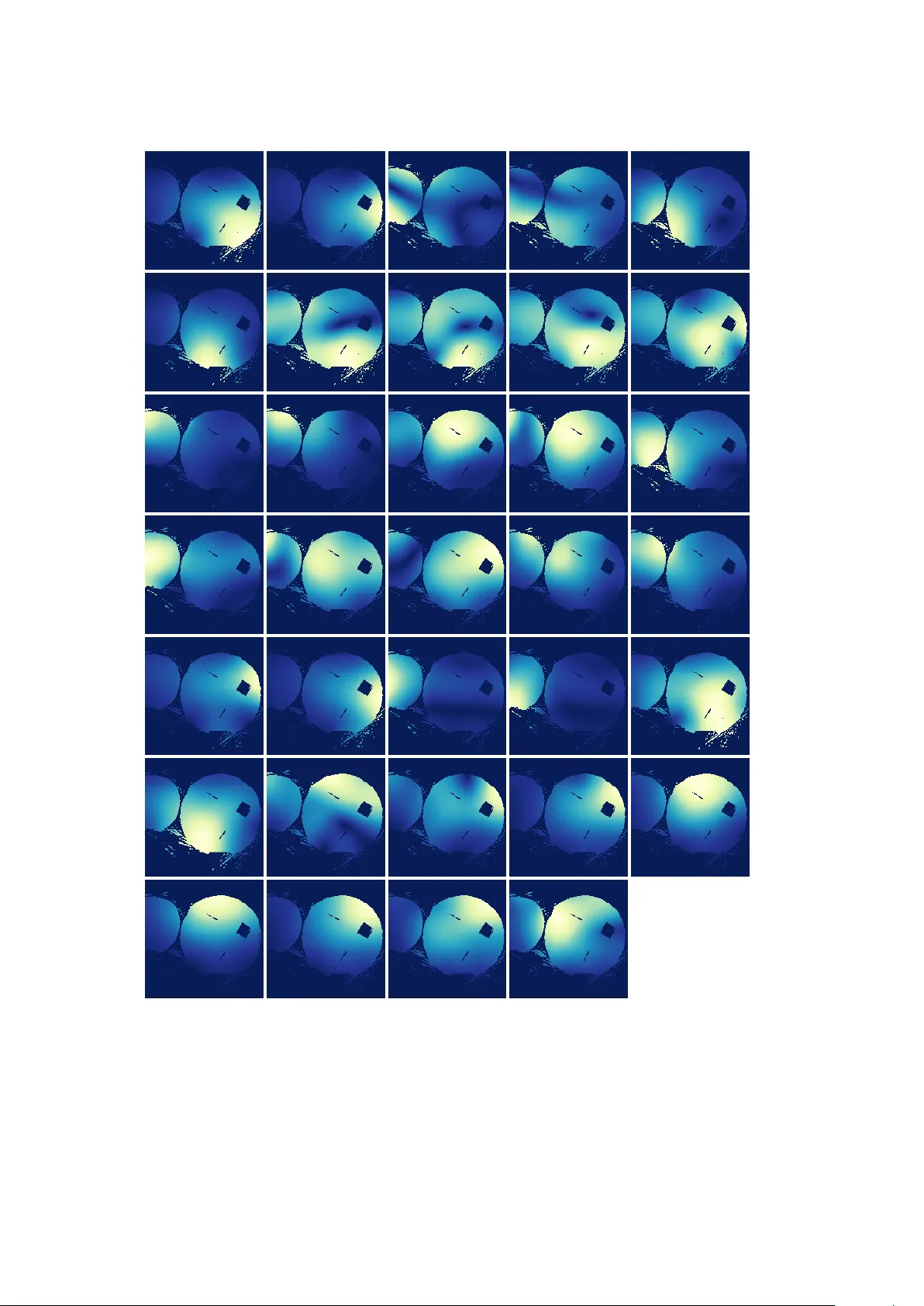
Fakultät für Physik Master’s Thesis V orbereitende Datenanalyse zur Rekonstruktion von Echtzeit-MRT -Daten Preparatory data analysis for the reconstruction of r eal-time MRI data prepared by Hans Christian Martin Holme from Soest at the Biomedizinische NMR Forschungs GmbH am Max-Planck-Institut f ¨ ur biophysikalische Chemie Date of Submission: 18th February 2016 First Referee: Prof. Dr . Jens Frahm Second Referee: Prof. Dr . Tim Saldi Contents 1. Introduction 1 2. Magnetic Resonance and Image Reconstruction 3 2.1. Magnetic Resonance Imaging . . . . . . . . . . . . . . . . . . . . . . . . . 3 2.1.1. Principles . . . . . . . . . . . . . . . . . . . . . . . . . . . . . . . 3 2.1.2. Radial FLASH . . . . . . . . . . . . . . . . . . . . . . . . . . . . . 8 2.2. Non-linear Inverse Reconstruction . . . . . . . . . . . . . . . . . . . . . . 11 2.3. Undersampling and Image Artifacts . . . . . . . . . . . . . . . . . . . . . 12 3. Methods 15 3.1. Data Acquisition and Processing . . . . . . . . . . . . . . . . . . . . . . . 15 3.1.1. Pre- and Postprocessing . . . . . . . . . . . . . . . . . . . . . . . 16 3.1.2. nlinv++ . . . . . . . . . . . . . . . . . . . . . . . . . . . . . . . . 16 3.2. Data Visualization . . . . . . . . . . . . . . . . . . . . . . . . . . . . . . . 18 4. Coil Compression 21 4.1. Principal Component Analysis . . . . . . . . . . . . . . . . . . . . . . . . 21 4.1.1. e PCA Algorithm . . . . . . . . . . . . . . . . . . . . . . . . . 21 4.1.2. Application in real-time MRI . . . . . . . . . . . . . . . . . . . . 22 4.2. Optimized Combination . . . . . . . . . . . . . . . . . . . . . . . . . . . . 25 4.3. Performance Evaluation . . . . . . . . . . . . . . . . . . . . . . . . . . . . 30 4.4. Discussion . . . . . . . . . . . . . . . . . . . . . . . . . . . . . . . . . . . 36 5. Coil Selection 37 5.1. Current Methods . . . . . . . . . . . . . . . . . . . . . . . . . . . . . . . 41 5.1.1. Manual Selection . . . . . . . . . . . . . . . . . . . . . . . . . . . 41 5.1.2. Xue et al. . . . . . . . . . . . . . . . . . . . . . . . . . . . . . . . 41 5.1.3. Grimm et al. . . . . . . . . . . . . . . . . . . . . . . . . . . . . . . 42 5.2. Sinogram-based Selection . . . . . . . . . . . . . . . . . . . . . . . . . . . 47 5.3. Discussion . . . . . . . . . . . . . . . . . . . . . . . . . . . . . . . . . . . 54 iii Contents 6. Summary and Outlo ok 55 A. Additional Figures 57 B. Sequence Parameters 61 Bibliography 63 iv Glossar y CT . . . . . . . . . . . . . computed tomography DFT . . . . . . . . . . . . discrete Fourier transform FID . . . . . . . . . . . . free induction decay FLASH . . . . . . . . . . fast low-angle shot FO V . . . . . . . . . . . . eld of view GP U . . . . . . . . . . . . graphics processing unit GRAPP A . . . . . . . . . generalize d autocalibrating partially parallel acquisition IRGNM . . . . . . . . . . iteratively regularized Gauss-Newton method MRI . . . . . . . . . . . . magnetic resonance imaging NLIN V . . . . . . . . . . non-linear inverse reconstruction NMR . . . . . . . . . . . nuclear magnetic resonance PCA . . . . . . . . . . . . principal component analysis PSF . . . . . . . . . . . . point spread function rf . . . . . . . . . . . . . . radio frequency SENSE . . . . . . . . . . sensitivity encoding SNR . . . . . . . . . . . . signal-to-noise ratio T 1 . . . . . . . . . . . . . spin-laice relaxation time v Glossary T 2 . . . . . . . . . . . . . spin-spin relaxation time T ∗ 2 . . . . . . . . . . . . . eective spin-spin relaxation time vi 1. Introduction Magnetic resonance imaging (MRI) is an important radiological technique for imaging sections or volumes in clinical and scientic seings. Starting fr om its introduction by Lauterbur [1] in 1973, it has evolved into a routine procedure. Be cause of the lack of ionizing radiation, its excellent so tissue contrast, and its wide variety of imaging modalities, it is now used in hospitals and research institutes worldwide . An inherent problem of MRI is its low spee d, since images are sampled line-by-line in Fourier space. is low inherent speed has practical implications, e.g. movement during the acquisitions degrades image quality , and dynamical processes impose requirements on image timing. erefor e, acceleration of MRI image acquisition has been a research focus since its beginning. A success in this drive for spe ed has b een the introduction of fast low-angle shot (FLASH) imaging in 1985[2 – 4], which r educed the imaging time from minutes to mer e seconds. is hastene d the integration of MRI into routine clinical use. Further sp eed im- prov ements based on FLASH MRI were possible by tackling the sampling: e introduction of multiple receiver coils, combined with parallel MRI [5], allows image r econstruction even from undersampled data. Pushing this undersampling further leads to the common trade-o of increased imaging spe ed at the cost of de creased signal-to-noise ratio (SNR). Nowadays, accelerated acquisition sequences coupled with sophisticated reconstruction algorithms to cope with the high undersampling have pushed this even further , with imaging times below 30 ms [6]. is enables the recording of MRI movies instead of still images. T ogether with modern computer hardwar e, this led to the introduction of real-time MRI, with both image acquisition and image reconstruction in real time. While holding great promise, r eal-time MRI also poses new challenges: e increased imaging spe eds, for example, lead to large volumes of data which, together with com- putationally intensive reconstruction algorithms, can diminish reconstruction spee ds. Furthermore, the high degree of undersampling can lead to unacceptable image artifacts. is thesis introduces and evaluates approaches for handling these two problems. Chap- ter 4 discusses coil compression methods for reducing the data volume, while a new coil selection algorithm for streak artifact reduction is introduced in Chapter 5. 1 2. Magnetic Resonance and Image Reconstruction is chapter provides a brief overview over nuclear magnetic resonance (NMR) and MRI, and also an introduction into the reconstruction technique used in this work. A more general introduction into MRI and the underlying physics is given in textb ooks like Bernstein, King, and Zhou [7] and Haacke et al. [8]. 2.1. Magnetic Resonance Imaging 2.1.1. Principles is section follows Chapters 1 and 9 of Haacke et al. [8]. MRI relies on the interaction of a magnetic moment µ with an external eld B 0 . e magnetic moment in this case is the nuclear magnetic moment, generated by the nuclear spin. e principal nucleus used in MRI is hydrogen in water , fat, and other organic molecules. For a hydrogen nucleus — a pr oton — in a magnetic eld B 0 , the Zeeman eect leads to an energy dierence between parallel and anti-parallel alignment of the spin, with alignment parallel to B 0 having lower energy . e energy dier ence is ~ γ B 0 , where ~ is the reduced P lanck constant and γ is the gyromagnetic ratio, a nucleus-dependent value. While this constrains the nuclear magnetic moment in the direction of B 0 to two possible values, there is no such restriction in the transversal plane orthogonal to B 0 . erefore , in analogy to a classical magnetic moment, the expectation value will start to precess around B 0 . e frequency of this pr ecession is called the Larmor frequency ω 0 with ω 0 = γ B 0 . In an extended object made up of multiple spins, since there is no phase coherence imposed on this precession, the transversal magnetic moments cancel out, leaving a bulk magnetization parallel to B 0 . Since the energy dierence b etween alignment parallel and anti-parallel to B 0 is small compared to the thermal energy at b ody temp erature, the population dierence between 3 2. Magnetic Resonance and Image Reconstruction the two states is also small — at 1 T , the population dierence is ab out 6 excess spins p er million [9, p. 36] — but it still leads to a macroscopic magnetization M 0 which is large enough for NMR eects. M 0 is given by [8, p . 5] M 0 = ρ 0 γ 2 ~ 2 4 kT B 0 , where ρ 0 is the number of protons per unit volume, k is the Boltzmann constant, and T is the temp erature. Precession of the macroscopic magnetization can be achieved by resonant e xcitation. e resonance condition is that the frequency of the magnetic excitation pulse B 1 ( t ) needs to be the Larmor frequency . For the commonly used nuclei and eld strengths this frequency is in the radio-frequency range, the excitation pulses are therefore commonly called radio frequency (rf ) pulses. e angle by which the magnetization is tipp ed is called the ip angle, and it depends b oth on the eld strength and duration of the rf pulse. e excitation pulse achieves its eect by two mechanisms: First, it will ip spins from the lower energy parallel to the higher energy anti-parallel state, thereby reducing longitudinal magnetization. Second, it will impose its phase onto the precession, thereby causing a non-vanishing transversal magnetization. Combined, this leads to a bulk magnetization that starts to precess and to tip over the duration of the rf pulse . Suppose an rf pulse is applied that tips the magnetization into the transversal plane (called a 90 ° -pulse). Directly aer this pulse, the bulk magnetization precesses in the transversal plane. is magnetization will induce a changing magnetic ux in nearby coils, which can be detecte d. e longitudinal magnetization will e ventually relax back into the equilibrium state. is can be understo od as the spins excited into the anti-parallel state ipping back into the parallel state. is is an exponential process characterized by the spin-laice relaxation time ( T 1 ). If the e quilibrium magnetization is M 0 , the longitudinal magnetization will recover accor ding to: M k ( t ) = M 0 1 − e − t T 1 . Furthermore, the dierent spins are not only ae cted by the external magnetic eld, but also by the magnetic elds pr oduced by other spins. is leads to slightly dierent Larmor frequencies for each spin, causing a loss of phase coherence calle d dephasing and thereby a loss of bulk transversal magnetization. is decay is characterized by the spin-spin relaxation time ( T 2 ), following M ⊥ ( t ) = M 0 e − t T 2 . T 2 is always shorter than T 1 , with typical values for T 2 on the order of 1 ms to 100 ms and for T 1 on the order of 100 ms to 1000 ms . Inhomogeneities of the static magnetic eld B 0 will lead to ev en faster dephasing, characterized by the eective spin-spin r elaxation time ( T ∗ 2 ) with T ∗ 2 < T 2 . 4 2.1. Magnetic Resonance Imaging Application of an excitation pulse to an object generates a decaying signal calle d free induction decay (FID ). An alternativ e way to cr eate a signal is by generating an echo. e basic setup is the same: a 90 ° -pulse is applied to tip the magnetization into the transversal plane, where they will dephase due to T 2 decay . By applying a second rf-pulse aer τ , this time a 180 ° -pulse, the magnetization stays in the transv ersal plane but it is r otated by 180 ° about an axis within the transversal plane; or alternativ ely , the phase of each spin is turned to its negative . is means that the spins that acquired excess phase between excitation and 180 ° -pulse now lag behind and vice versa. erefor e, the spins rephase at t = 2 τ and an echo forms. is is called a spin echo. e str ength is still aenuated by e − 2 τ / T 2 due to T 2 decay . Figure 2.1a shows a diagram of spin echo formation. An echo can also b e generated without using a se cond rf pulse. For this, the spins are rst dephased by applying a gradient and then rephased by applying a gradient with the same strength but with the opposite sign. e echo is formed at the instant where the combined area under both gradients equals zero. e r esulting echo is called a gradient echo or gradient-recalled echo. In contrast to a spin echo, the gradient echo is aenuate d by the shorter T ∗ 2 , since the magnetic eld inhomogeneities are not canceled out by phase inversion. Figure 2.1b depicts gradient echo formation. (a) (b) Figure 2.1: Diagram for (a) spin echo and (b) gradient echo formation. For the spin echo in (a), no gradients are necessar y: aer an inital 90 ° rf-pulse, the FID signal begins to decay . Applying a 180 ° -pulse aer T E / 2 leads to a spin echo aer T E . e gradient echo in (b) shows the same FID decay aer the 90 ° -pulse, but the spins are then dephased and rephased with an applied gradient. Ploed here is the gradient strength over time. Diagrams adapte d from [10]. For generating an image, it is necessary to relate spatial position and signal. e idea in MRI is to use magnetic gradient elds and exploit the linear dependence of the Larmor frequency on eld strength. is can be understood most easily in the one-dimensional 5 2. Magnetic Resonance and Image Reconstruction case: By applying a linear gradient G ( t ) in x -direction the total magnetic eld becomes B ( x , t ) = B 0 + x G ( t ) . is changes the local Larmor frequency to ω ( x , t ) = ω 0 + ∆ ω ( x , t ) with ∆ ω ( x , t ) = γ x G ( t ) . is is called frequency enco ding, since the position of the spins is hereby related to their precession frequency . e signal s ( t ) in MRI depends on the eective spin density 1 ρ ( r ) and the phase of the precessing spins ϕ ( r , t ) [8, p. 141], s ( t ) = ρ ( r ) e i ( ω 0 t + ϕ ( r , t )) d 3 r where ϕ ( r , t ) = − t 0 ω ( r , t ) d t . For a one-dimensional object ρ ( r ) = ρ ( x ) δ ( y ) δ ( z ) , the signal aer frequency encoding and demodulation of ω 0 becomes s ( t ) = ρ ( x ) e − i t 0 ∆ ω ( x , t ) d t d x . By noting that t 0 ∆ ω ( x , t ) d t = γ z t 0 G ( t ) d t and introducing 2 π k ( t ) : = γ t 0 G ( t ) d t , the time dependence can be made implicit in k : s ( k ) = ρ ( x ) e − 2 π i k x d x . Here, s ( k ) is the Fourier transform of ρ ( x ) , and so can be inverted to obtain the spin density from a frequency-enco ded measurement ρ ( x ) = s ( k ) e 2 π i k x d x . e k is naturally identied as a v ector in the r e ciprocal or Fourier space, called k -space in MRI. e temporal evolution of the gradient determines k ( t ) , which is referred to as the trajector y in k -space. In practice, the signal cannot be recorded continuously but is sampled at discrete points instead. e gradient echo introduced ab ove is an e xample of a trajector y that can be used to sample a region around the center of k -space: e rst dephasing gradient moves the sampling point away from the k -space center for a time τ . If the subsequent rephasing gradient has the same gradient strength but twice the duration, a symmetric line around the k -space center will be encoded in the signal. If it is sampled during the rephasing gradient, this symmetric k -space line can b e used to reconstruct the object by 1D Fourier transformation. For two-dimensional objects, there are several encoding schemes. One is radial encod- ing, which will be e xplained in Se ction 2.1.2, another is Cartesian encoding. For Cartesian encoding, parallel lines are sample d in k -space. Each line of k -space is measured with frequency encoding in a separate repetition, so with a separate excitation pulse. T o mea- sure shied lines in k -space an additional gradient, called phase-encoding gradient, is applied between excitation and frequency encoding. e direction of this gradient has 1 e eective spin density is the plain spin density ρ 0 with all constants absorbed into it. is simplies the resulting expressions. See p . 141 of Haacke et al. [8] for an exact denition. 6 2.1. Magnetic Resonance Imaging to be orthogonal to the frequency-encoding direction. is gradient leads to a phase shi in real space, which in turn implies a translation in k -space. For a certain choice of line separation, gradient str ength and sampling rate , the measured samples will lie on a Cartesian grid in k -space, hence the name Cartesian encoding. e reconstruction is simply a two-dimensional discrete Fourier transform. Figur e 2.2a shows a diagram of a Cartesian encoding scheme. For imaging a slice of a three-dimensional obje ct, slice selection can be use d. Here, a gradient orthogonal to the desired slice is applie d during the excitation pulse. If the gradient is such that it is zero in the desired slice, the Larmor frequency changes ev ery- where except in the slice itself, so the resonance condition is only fullled in the slice and only it will be excited, yielding eectively a two-dimensional object for imaging. For three-dimensional imaging, either phase encoding can be extended in the third direction, or slice selection can be use d to image each slice serially . Image reconstruction in MRI invariably involves discr etization, which introduces the problem of sampling: the imaging procedures described above can only work if proper sampling is taken into account, with the sampling rate subject to the Nyquist criterion and the maximum k -space extent determining the resolution [8, Ch. 12]. Sampling and associated artifacts are discussed in more detail in Section 2.3. In general, the choice and timing of imaging gradients and rf pulses can modify the contrast of MRI images to an astonishing degree, with far more possibilities than could be describe d here. An o verview over a large number of MRI sequences can be found in Bernstein, King, and Zhou [7]. Modern MRI uses multiple receive coils. An advantage is the increased signal-to-noise ratio (SNR), which comes from smaller coils which can be placed closer to the object. Multiple coils with o verlapping sensitivity proles can co ver the same volume as a single large coil. But, instead of the single global image reconstructed ab ove , each coil contains information from only part of the object. erefore, a combined image is normally calcu- lated as the r oot-sum-of-squares of the individual coil images [11]. A further advantage of multiple receive coils is the possibility of parallel imaging: 2D and especially 3D images require a large number of repetitions, leading to long measurement times. e idea of parallel imaging is to sp eedup this process by using the spatial information contained in the sensitivity variation of the coils to replace time-consuming spatial encoding. In Cartesian imaging, the spe edup comes from skipping phase-enco ding lines. is leads to reduced coverage of k -space called undersampling. Sp ecial reconstruction te chniques are necessary to recover usable images, since naive Fourier reconstruction with skippe d phase-encoding lines leads to aliasing in the images. Common parallel imaging techniques 7 2. Magnetic Resonance and Image Reconstruction include sensitivity encoding (SENSE)[12], generalized autocalibrating partially parallel acquisition (GRAPP A)[13], and the non-linear inv erse reconstruction (NLINV) use d in this thesis and described in Section 2.2. An overview ov er parallel imaging techniques can be found in Deshmane et al. [5]. 2.1.2. Radial FLASH FLASH e most important pulse sequence in this thesis is radial fast low-angle shot (FLASH). FLASH is a technique for rapid acquisition of MRI images, introduce d in 1985 by Frahm et al. [2]. e acquisition scheme described ab ove uses 90 ° -pulses, which maximizes the usable transversal magnetization for imaging, but also ne cessitates waiting for full T 1 recovery before the next excitation. FLASH uses gradient echo es and small angle pulses with ip angles smaller than 15 ° . Combined with continuous imaging, this leads to the development of a steady state, with the longitudinal magnetization lost to rf excitation being recovered thr ough T 1 relaxation during the sequence. With continuous imaging, even the transverse phase coherence does not relax completely . is needs to be rectied, either by applying strong gradients, called crusher gradients, which completely dephase the transverse magnetization; or by rf-spoiling, which applies a phase oset onto each excitation pulse, thereby suppressing the buildup of a steady state of the transversal magnetization [8, p. 500f]. For fast imaging, rf spoiling is preferr e d, since it avoids the time-consuming crusher gradients. With rf-spoile d FLASH, repetition times on the order of 2 ms are possible. e steady state which is built up during a FLASH acquisition also dictates the contrast: Since this steady state is T 1 -dependent, FLASH-acquisitions with short repetition times and short echo times on the order of milliseconds, like the sequences used for real-time MRI, will show T 1 -weighting, with shorter T 1 appearing brighter . Radial Imaging Radial encoding is the other dierence to current routine MRI. Instead of recording lines on a Cartesian grid in k -space, lines through the k -space center are recorded in a paern similar to spokes on a wheel. While it is not necessar y , the radial trajectories in this thesis use equiangular spacing. A diagram of a radial traje ctory is shown in Figure 2.2b. It is immediately obvious that radial trajectories sample k -space non-uniformly . is is a problem in the outer regions of k -space which contain high resolution information: 8 2.1. Magnetic Resonance Imaging (a) (b) Figure 2.2: Sequence and k -space diagrams for (a) Cartesian and (b) radial encoding. e dashed gradient line in the se quence diagram corresponds to the dashed k -space line in the k -space diagram. Both contain an α -pulse and a slice selection gradient. In (a) Cartesian encoding, the same frequency- encoding gradient is use d during readout in all lines, only the phase- encoding gradient changes. In (b) radial enco ding, both x and y gradients use frequency encoding, so both are present during readout. Diagrams adapted from [10]. 9 2. Magnetic Resonance and Image Reconstruction e lower sampling in this region means that radial trajectories need to measure mor e lines to achieve similar resolution to Cartesian traje ctories. e higher sampling of k - space close to the center , however , is an advantage over Cartesian imaging, since it leads to reduced motion sensitivity . Another advantage is the absence of a phase-enco ding gradient, enabling shorter echo times and, together with FLASH, faster repetition rates. Radial imaging also allows uniform readout oversampling. is means faster sampling of the MRI signal, commonly doubling the sampling rate, thereby enlarging the eld of view (FO V) without aecting the resolution. e aliasing artifacts arising fr om discrete and nite sampling of k -space are hereby moved further from the region of interest. Aer reconstruction, the excess part of the FO V is discarded again. Since it is done during sampling, no additional imaging time is neede d, and while readout oversampling is limited to the frequency-encoding direction in Cartesian imaging, no such limitation exists in radial imaging. Reconstruction also changes with radial encoding: A simple inverse 2D Fourier trans- form is no longer possible. Instead, there ar e two main ways to reconstruct images: Projection reconstruction and gridding. Pr oje ction reconstruction relies on the Fourier slice theorem, which states that the 1D Fourier transform of lines through the origin of k -space are the projections orthogonal to the line . With this, each measured line can be Fourier transformed, mapp ed to an angle, and then reconstructed with methods like ltered backpr ojection or other techniques common in compute d tomography (CT). Grid- ding is an alternative approach, where the radial spokes are r esampled onto a Cartesian grid, which is then 2D Fourier transformed. e most important advantage of radial trajectories is, howev er , the p ossibility of uniform ( azimuthal) undersampling: In Cartesian MRI, only the phase-encoding dir e ction can be undersample d reasonably; undersampling the frequency-encoding direction does not lead to an appreciable de crease in measurement time. But the non-uniform sampling achieved by skipping phase-encoding lines limits the degree of undersampling that can be used. With radial sampling, since each spoke samples b oth low and high k -space regions, measuring fe wer spokes while retaining equiangular spacing leads to uniform undersampling. For real-time MRI, where very high undersampling factors are used, this uniform undersampling also helps with temporal resolution: In Cartesian MRI, the central k -space which contains overall obje ct shape is only measured once per frame. In radial acquisition, each spoke measures the k -space center , so each sp oke contains equally important data. Undersampling and related image artifacts is describ ed in more detail in Section 2.3. e application of radial FLASH for real-time MRI is described, for example, in Zhang, Block, and Frahm [14] and Uecker et al. [6]. 10 2.2. Non-linear Inverse Reconstruction 2.2. Non-linear Inverse Reconstruction e most important ingredient for real-time MRI is the non-linear inverse r econstruction (NLIN V) introduced by Uecker et al. [15] in 2008. A closer look at the signal in parallel MRI is necessary here. For a coil array with N coils, the signal in the j th coil is given by [10, p. 25]: s j ( t ) = ρ ( x ) c j ( x ) e − 2 π i k ( t ) x d x + n ( t ) with the pr oton density ρ , the comple x-value d spatial sensitivity proles c j , receiver noise n , and the used time-dep endent k -space trajector y k ( t ) . For MRI reconstruction, this has to be discretized and be comes ([10, p. 32]) s = P k F C ρ + n (2.1) where C is the multiplication with the spatial sensitivity proles ( coil proles), F is the discrete Fourier transform, and P k is the projection onto the trajector y . If the spatial sensitivity proles ( or coil proles) are kno wn, this can be regarded as a linear inverse problem ([10, Ch. 3.4.2]) y = A x + n with A = P k F C . e parallel imaging techniques mentioned in Section 2.1.1 can b e understood as tw o-step approaches, rst estimating the coil pr oles from calibration data and then solving this linear inverse problem. A problem with the two-step approach is that is does not use the available data optimally . e idea of NLIN V is to jointly estimate image content and coil proles, enabling beer use of the available data and leading to higher image quality . Here, MRI is understoo d as a non-linear operator equation F ( x ) = y , with x = ρ c 1 . . . c N (2.2) with an operator F that maps the unknowns, the proton density ρ and the coil prole c i for each of N coils, to the measured k -space data y . For large undersampling factors both the linear and the non-linear parallel imaging problems b ecome ill-conditioned, leading to noise amplication. erefor e, r egularization is introduced to curtail the noise amplication. In this thesis, the iterativ ely regularized Gauss-Newton method (IRGNM) is used to the solve the non-linear problem. e operator F takes the following form (compare 11 2. Magnetic Resonance and Image Reconstruction Equation (2.1)): F : x 7→ P k F c 1 ρ . . . P k F c N ρ (2.3) An obvious pr oblem is the insucient separation b etween c i and ρ : multiplying each c i by any complex function and dividing ρ by the same function leaves the pr oduct unchanged. Even the extreme case of all proton density information in the coil proles c 0 i = c i ρ , ρ 0 ≡ 1 is possible without further constraints. Since coil proles ar e generally smooth, this problem can be solved with a regularization term p enalizing high k -space frequencies in the coil proles. As further r egularization, the distance to an initial guess can be used. In the conte xt of real-time MRI, a slightly dierent approach is useful: As long as the frame rate is suciently high to resolve the dynamics of the measured obje ct, subsequent frames will be very similar . So instead of a penalty on the dierence to an initial guess, the dierence to the preceding frame is penalized, constituting a form of temp oral regularization. Constraining the reconstruction through prior knowledge in this way is necessary to recover the data missing because of undersampling. A more detailed description of the IRGNM and its application to MRI can be found in Chapter 5 of Uecker [10] and in Uecker et al. [15]. e implementation of NLIN V use d in this thesis is describ ed in Section 3.1.2. 2.3. Undersampling and Image Artifacts Undersampled MRI acquisitions are the basis of the real-time MRI used in this thesis, because of the p ossibility for tremendous speedup. T o understand undersampling, su- cient sampling must be introduced rst. For radial sampling this leads to the following statement: For a quadratic eld of view of length L and a desired resolution ∆ x determined by the highest sampled frequency k max = 1 2 ∆ x in k -space, the Nyquist criterion states that the angular spacing ∆ ϕ between the spokes has to fulll [7, p. 906] k max ∆ ϕ ≤ 1 L . Or equivalently the number of sp okes n spokes has to fulll n spokes ≥ π Lk max (2.4) Compared to the needed numb er of phase-encoding steps n phase in Cartesian sampling n spokes = π 2 n phase (2.5) holds, so approximately 57 % mor e excitations are necessar y [7, p. 906]. 12 2.3. Undersampling and Image A rtifacts For real-time MRI, full Nyquist sampling per frame is too slow , so far fewer spokes are generally recorded. e eects that this undersampling has on images can be understo od using the point spread function (PSF). It is the image of a single p oint produce d by the imaging pr ocess under consideration. So the image of an extended object is the convolution of this object with the PSF. In MRI, the PSF is determined by the k -space sampling paern. Figure 2.3a shows the PSF for a fully sampled radial acquisition. e PSF consists of a central lobe determining the shape of an imaged point, surrounded by a region where it is close to zero (called the artifact-free region), in turn surrounded by artifact-generating side-lobes. In Figure 2.3a, the artifact-free region covers the entire FO V. Using only half the Nyquist-dictated number of spokes as in Figure 2.3b leads to larger side lob es covering the e dge of the FO V, while even lower numb ers of sp okes almost completely eliminate the artifact-free region (Figures 2.3c and 2.3d). e artifacts generate d by this imperfe ct PSF are mostly streak artifacts, which are generated by each pixel of the object at a distance determined by the extent of the artifact-free region. For real-time MRI, it is common to record less than 20 spokes per frame, leading to a large problem with streak artifacts (Figure 2.3d). Since the image is the convolution of the PSF with the object, high intensity regions of the object will generally lead to more intense streak artifacts. e problem of artifacts is partly mitigate d by NLIN V, through temporal regularization: the PSF and therefore the streak artifacts are dierent in subsequent frames, so temporal regularization leads to a dampening. But since streak artifacts are still a signicant problem in some real-time MRI acquisitions, another possible mitigation strategy based on coil selection is the subject of Chapter 5. 13 2. Magnetic Resonance and Image Reconstruction (a) 403 spokes (fully sampled) (b) 201 spokes (c) 85 spokes (d) 17 spokes Figure 2.3: Absolute value of simulated p oint spread functions for (a) 403, (b) 201, (c) 85, and (d) 17 spokes. e FO V size is 256 × 256. According to Equation (2.5), full Nyquist sampling r equires more than 402 spokes. 17 and 85 spokes were chosen since those ar e common values for the number of spokes per single frame and per full frame in r eal-time MRI (for a denition of the terminology see Section 3.1). 14 3. Methods 3.1. Data Acquisition and Pr ocessing All data used in this thesis was acquired using a MAGNET OM Primsa t system (Siemens Healthcare, Erlangen, Germany) at a eld strength of 3 T . For cardiac and abdominal measurements a 32-channel coil array was used, consisting of anterior and p osterior 16-channel arrays. For head measurements a 64-channel head coil was used. Phantoms used either coil array . A radial FLASH sequence developed in the insitute was used for acquisition. is sequence uses a turn-based paern, where a set of n spokes spokes is acquired for each frame. For the subsequent frame, this paern is rotated by 2 π / n turns · n spokes , so that aer n turns frames the paerns overlap again. is is illustrated in Figure 3.1. n turns frames taken together , containing all spoke orientations, are called a full frame . Acquisition parameters for the datasets used in this thesis can be found in T able B.2 in Appendix B, while descriptions of the datasets are gather ed in T able B.1. Dataset labels are typeset in small capitals (e .g. Head1 ) so that they can be quickly identie d. Figure 3.1: Diagram showing an acquisition with 5 sp okes and 3 turns. e numbers next to the spokes sho w the order in which they ar e acquired. Between spokes, there is an angle of 360 ° / n spokes (here: 360 ° / 5 = 72 ° ), between turns an angle of 360 ° / n spokes · n turns (here: 360 ° / 5 · 3 = 24 ° ). e ( n turns + 1 ) th turn is again identical to the rst turn. 15 3. Methods 3.1.1. Pre- and Postprocessing ere are several pr e- and postprocessing steps applied to the measured data. First is a gradient delay correction using the rst full frame: due to imperfect gradient timing in the MRI system, the actually measured k -space trajectory deviates from the expe cted trajector y . is can partly be corrected by gradient delay correction. e procedure is described in detail in Chapter 4 of Untenberger [16]. en, the data is compressed by a principal component analysis (PCA) to few er channels. is procedure is describe d in Chapter 4. e corrected and compressed data is then interpolated on a square Cartesian grid in a procedure called gridding , describe d, for example, in Chapter 13.2 of Bernstein, King, and Zhou [7]. For b eer accuracy of the interp olation, the Cartesian grid is chosen with a 1 . 5 times higher sample density than the originally sampled k -space data. is is called overgridding . e gridded frames are then reconstructed using NLIN V. e postprocessing steps dep end on the application. For anatomical real-time MRI, a pixelwise temporal median lter is applied: Each pixel in frame n is replaced by the median of the same pixel in the frames n ± b n turns 2 c . A non-local means lter for image denoising, described in Klosowski and Frahm [17], is applied next. For other applications, dierent postprocessing steps are needed. For phase-contrast ow imaging the phase dierence map needs to be calculated, for example. All pre- and p ostprocessing steps are available in two implementations: a MATLAB 1 implementation and integrated in nlinv++ . e MATLAB implementation is used for testing and implementing new techniques, while nlinv++ can be used directly on the MRI scanner . 3.1.2. nlinv++ nlinv++ is a C++ program wrien in the institute. It can be used online (i.e. on the MRI scanner) and oine. e online version is running as a “bypass server” , so instead of forwarding the data to the vendor-supplied reconstruction pipeline, it is send to the custom reconstruction pipeline instead. e reconstructed images are then wrien back to the scanner , yielding seamless integration. Oine, nlinv++ can be use d to reconstruct previously measur ed data again. nlinv++ is itself implemented as a pipeline. It consists of ve pip eline stages, each running in its own thr ead with an additional thread for the contr olling stage. e ve pipeline stages are: datasource , preprocessor , reconstructor , postprocessor , and data- sink . e stages are connecte d by channels, which are implemented as thread-safe 1 MATLAB is a registered trademark of e MathW orks, Massachuses, USA. 16 3.1. Data Acquisition and Processing type-erased lists, so any kind of message may be passed along the pipeline. Each pipeline stage decides on the appropriate action base d on the type of this message 2 . Since the NLIN V algorithm contains Fourier transforms and matrix-products of large matrices, the reconstructor stage uses graphics processing units (GP Us) to accelerate computation. nlinv++ is running on dedicate d Supermicro SuperSer ver 4027GR- TR system with the Ubuntu 14.04 operating system, 2x Intel X e on Ivy Bridge E5-2650 main processors, 8x N VIDIA GTX Titan Black (Kepler GK110) GP Us as accelerators, and 128 GiB main memory . e setup is as follows: the controlling main thread starts up and sets up the congura- tion. It then starts up each of the pipeline stages: datasource It reads in the raw measured data, either from a le or from a pipe connected to the scanner . It buers data until enough data for one frame has b een read and then sends it on. preprocessor It receives the raw data from the datasource one frame at a time. It uses the rst full frame as calibration data to calculate the gradient delay values and the coil compression matrix. It applies gradient delay correction, coil compression and gridding to each frame. Coil compression is discussed in more detail in Chapter 4. reconstructor e reconstructor is the only stage that is itself multithreaded, com- monly using up to 4 threads. Each thread is identical, and each reads its input from the common channel coming from the preprocessor . Since 8 GP Us are available, each of n threads reconstructor threads distributes its data onto b 8 n threads c GP Us. Each thread independently reconstructs its frame and places it in the channel to the postprocessor . postprocessor Receives reconstructed frames from the reconstructor and applies ap- propriate postprocessing to them. In most cases, that means temporal median and non- local means ltering. For phase-contrast ow MRI for example, it includes calculation of the phase-contrast map. datasink Receives postprocessed images and writes them to le. Since the reconstruc- tor is multithreaded, it might receive frames out-of-order . In that case, it buers the out of order frames while waiting for the next in-or der frame. 2 e type is only erase d inside the channels, it is recovered in the pipeline stages to decide on the action to be taken. 17 3. Methods Once all data has been read, the datasource produces a finished message. Each subse- quent pipeline stage that receives this message produces its own finished message and exits as well. e datasink , aer having wrien all output data, produces a finished message for the controlling main thread. is nal message acts as a control that the reconstruction nished successfully . 3.2. Data Visualization e 2D images in this thesis are created using arrayShow 3 . Unless otherwise indicated, images are individually windowed. is ensures that comparisons b etween images are not unduly inuenced by , for example, dierences in total signal content. Furthermore, since the data analyzed in this thesis stems from real-time MRI acquisitions, they are properly understood as movies rather than still images. erefore , r epresentative individual frames were selected for this thesis. Figure 3.2 shows the colormaps use d in this thesis. For ease of identication, the colormap in Figure 3.2a is used to directly repr esent complex data, while the colormap in Figure 3.2b is used when showing the magnitude of comple x data. A plain grayscale colormap is used for purely real data. e comparison of dierent methods in this thesis is done by visual inspe ction of images, or by inspecting their dierence. is is done since no generally accepted criterion for quantication of image quality exists in MRI, and since medical images are traditionally interpreted through visual inspe ction by physicians. Furthermore, the postprocessing lters described in Section 3.1.1 ar e not used on the images, so that the comparison is not unduly inuenced by them. 3 https://github.com/BiomedNMR/arrShow , arrayShow is a MATLAB image viewer for multidimensional ar- rays, with a focus on MRI images. 18 3.2. Data Visualization (a) Complex colormap (b) Magnitude colormap Figure 3.2: Colormaps used in this thesis. Both (a) and (b) show the complex unit disk. (a) shows the colormap used for directly representing complex-valued data, with hue indicating phase angle and brightness indicating absolute value. (b) shows the colormap used for representing the magntidue of complex data. e colormap in (a) is the standard colormap of arrayShow for com- plex data, while the colormap in (b) is the YlGnBu r (“yellow , green, blue, rev ersed”) colormap from the matplotlib project, optionally available in arrayShow . Purely real data is visualized with a grayscale colormap. 19 4. Coil Compression A challenge in modern MRI is the large amount of measurement data that can b e acquired with current systems. Arrays of 32 or 64 coils ar e in routine use today , with even larger numbers of coils in consideration[18]. e use of very fast imaging techniques in real-time MRI exacerbates this problem. One advantage of multiple receiver coils is the possibility of parallel imaging for impro ved image quality and faster acquisition. e drawback is increased computation time. A way to addr ess this problem is coil compr ession, that means nding a smaller approximation of the data that still captures as much of the containe d information as possible. One possibility is combining the measured coils into a smaller set of “virtual coils” , which is the approach taken here. One very fast approach is the use of linear combinations of coils, calculated from some initial calibration data. is enables the use of the once calculated compression op erator on new data as it is coming in, in a way suitable for online use. Furthermore, the channel compression can b e represented as a matrix product with the incoming data, which is advantageous be cause of the wide availability of highly optimized matrix-matrix-product routines. Especially the ease of online use is the reason why a linear method was chosen for the current nlinv++ implementation, namely PCA. 4.1. Principal Component Analysis Principal component analysis (see [19] for a general introduction) is a te chnique for dimensionality reduction and feature extraction used in statistics. Here, the dimensionality reduction is the important characteristic. 4.1.1. The PCA Algorithm e input of the PCA algorithm is the ungridded raw data of the rst full frame from scanner . is data consists of the measured samples for each line for each coil, so it is an array of dimensions n coils × n S × n samples , which for PCA is treated as a matrix of 21 4. Coil Compression dimensions n coils × n S · n samples . Here , n S = n spokes · n turns is the number of spokes in a full frame. 1. T ake the input matrix A of size n coils × n S · n samples and calculate the n coils × n coils matrix cov ( A ) : = A ∗ · A , where ∗ is the conjugate transpose operation. cov ( A ) is related to the covariance matrix of A, but diers in two important aspects. First, the covariance matrix requires the columns of A to have zero mean. is is not guaranteed for MRI data. e column means are, how ever , close enough to zero to have negligible inuence on the method. Second, the covariance matrix needs to be scaled by 1 / n samples , which cov ( A ) is not. 1 2. Find an eigenvalue decomposition of cov ( A ) , that means a unitary transformation matrix I and a diagonal matrix Λ so that cov ( A ) = I ∗ · Λ · I . Λ contains the eigenvalues of cov ( A ) on its diagonal, and all eigenvalues are real since cov ( A ) is a normal matrix 2 . 3. Jointly permute I and Λ so that the eigenvalues on the diagonal of Λ are in descend- ing order . 4. Use the rst n pc columns of I as the compression matrix, wher e n pc is the desired number of principal components. is metho d can be understoo d in the following way: By applying I to the input data it is transformed into a dierent coordinate system. In this system, the diagonal entries of Λ are a measure of the variation contained in each direction. e variation contained in the i th direction can be calculated as Λ i i / tr ( Λ ) , where tr () is the trace. So the rst n pc columns of I are a transformation matrix which retains n pc i = 0 Λ i i / tr ( Λ ) of the variation in A . is normalization with tr ( Λ ) is the reason why it is enough for the eigenvalues of Λ to be proportional to the covariances. 4.1.2. Application in real-time MRI For real-time MRI, the PCA algorithm is applied as a prepr o cessing step. In the prepro- cessor stage (see Section 3.1.2 for a discussion of the pipeline stages), the data of the rst full frame is use d as input for the algorithm. In the current implementation, n pc = 10, that is the rst 10 principal components are use d. is is a heuristically obtained, conservative 1 So cov ( A ) can only be proportional to the covariance matrix. However , this is sucient, as will be explained later . 2 A matrix M is normal if M · M ∗ = M ∗ · M , which is obviously fulllled for cov ( A ) 22 4.1. Principal Component A nalysis value [20, Ch. 6.3]. Images for comparison between n pc = 10 and n pc = n coils are shown in Figure 4.1. ere are se veral shortcoming of this approach: 1. It is indep endent of the image under consideration. Some images, especially of phan- toms, can naturally be described by fewer comp onents. Furthermore , the number of imaging coils is not taken into consideration. Using 10 principal components will have vastly dier ent results when using e.g. a 12-channel compar ed to a 64-channel head coil. 2. 10 only has 2 and 5 as factors. When distributing coil data onto accelerators for reconstruction (as describ ed in Section 3.1.2), this might lead to some accelera- tors containing more coil data to calculate than others. is will slow down the accelerators having to do more work, and thr ough synchronization between the accelerators slow down the whole r econstruction. 3. PCA nds “virtual coils” (dir e ctions) of highest variance. But this is not necessarily optimal for MRI: PCA will favor areas of high signal intensity at the expense of areas of lower intensity , creating not only non-uniform image appearance, but it can also lead to higher noise levels, since the coils with high sensitivity in the regions of low intensity will be weighted less. is eect, of course, is less pronounced at higher numbers of principal components. erefore , an optimize d coil compression algorithm was investigated in this thesis, in order to lo wer the number of necessar y principal components and thereby impr ove reconstruction speeds. 23 4. Coil Compression (a) n pc = full (b) n pc = 10 (c) n pc = full ( d) n pc = 10 (e) n pc = full (f ) n pc = 10 Figure 4.1: Comparison of using 10 principal components vs. using the full dataset for a water phantom ( Phan1 ) (a) – (b), a sagial slice through a human head ( Head1 ) (c) – (d), and a two-chamber view of a human heart ( Heart1 ) (e)– (f). e dierence in image quality is negligible. As an example Figure 4.2 shows the magnitude of the complex dier ence beween (c) and (d). 24 4.2. Optimized Combination Figure 4.2: Magnitude of the complex dierence between Figures 4.1c and 4.1d, shown as an example . Since the image is mostly noise with only lile structure in the high intensity regions, it can be concluded that the PCA compression to 10 coils does not impact image quality too much. 4.2. Optimized Combination In order to address these shortcomings of PCA for MRI, Buehrer et al. [21] have introduced an optimized coil compression algorithm for SENSE MRI [12]. A MATLAB implementation adapted for real-time MRI was already available in the institute 3 , and was use d for evaluation of the method. e optimized algorithm tries to over come some of the shortcomings of plain PCA, especially the non-uniform image appearance and the possible noise enhancement by using the coil proles as weighting. Figures 4.3 to 4.5 show the dierent steps of the algorithm applied to a water phantom dataset ( Phan1 ). 1. Input to the optimized algorithm are the n pixels × n pixels proton density R (Figure 4.3a) and the n pixels × n pixels × n coils coil sensitivity proles C (Figure 4.4) of a nished NLIN V run. Generate a n pixels × n pixels weighting matrix W with ∀ i , j W i j = 1. 2. Only consider pixels of moderately high image intensity . e threshold for this was set at 5 % of the maximum intensity: Set W to zero at { ( i , j ) | R i j < min ( R ) + 0 . 05 · ( max ( R ) − min ( R )) } (Figure 4.3b). 3. Calculate the combined sensitivity matrix S : S i j = n coils c = 1 k C i jc k 2 . 3 W rien by Soeren W olfers as part of an internship program. Because of the limited duration of the internship, no performance evaluation was done at that time. 25 4. Coil Compression 4. Normalize coil sensitivity in each pixel, i.e. divide W at each point ( i , j ) by S i j (Figure 4.3c). 5. Only considers pixels of mo derately high combined coil sensitivity . Here, the same threshold of 5 % of the maximum was chosen: Set W to zero at { ( i , j ) | S i j < min ( S )) + 0 . 05 · ( max ( S ) − min ( S )) } (Figure 4.3d). 6. Calculate weighted coil sensitivities: C w i jc = C i jc · W i j (Figure 4.5) 7. Transpose and interpret the n pixels × n pixels × n coils weighted coil sensitivities matrix C w as a n coils × n 2 pixels matrix and use the PCA algorithm describ ed in Se ction 4.1.1. is algorithm takes some insights into account. First, by using the proton density and coil sensitivity proles, it is possible to e xclude irrelevant pixels in the calculation. Furthermore, to generate more uniform image intensity and noise levels, the coil proles are normalized prior to PCA compression. A disadvantage of this method is the ne ed for the output of a nished NLIN V run. 26 4.2. Optimized Combination (a) (b) (c) (d) Figure 4.3: Visualization of dierent steps of the optimized algorithm. (a): magnitude of the input proton density R . (b) – (d): weighting matrix W aer (b) 5 % thresholding of the pr oton density , (c) normalization with the combined sensitivities, (d) 5 % thresholding of the combined sensitivities. For this dataset this last step leaves W unchanged, since the combined sensitivities pass the threshold at ev ery nonzero pixel. 27 4. Coil Compression Figure 4.4: Complex-valued input coil proles C for the optimized algorithm. 28 4.2. Optimized Combination Figure 4.5: W eighted coil proles C w of the optimized algorithm, use d as input for regular PCA. 29 4. Coil Compression 4.3. Performance Evaluation Since the optimized algorithm has not already been added into nlinv++ , the performance evaluation was strictly done oine, using MATLAB . Routines implementing data reading and preprocessing (including gradient delay correction and gridding) were already available. For the reconstruction, a modied version of nlinv++ was wrien as part of this thesis, which allows the input of data prepr ocessed in MATLAB and only uses the reconstructor and datasink stages describe d in Section 3.1.2. is was done to prev ent subtleties in the reconstruction from inuencing the results of the e valuation. Figures 4.6 to 4.10 provide an overview of the improvement that can b e expecte d from using the optimized compression algorithm over plain PCA. As can be seen, for most datasets the improv ement is limite d to lo w numbers of principal components (2 and 4); for 8 and 10 comp onents, the dierence in all datasets is very small. In the head datasets (Figures 4.6, 4.8 and 4.9) for 2 principal components, the improv e- ment in image intensity uniformity can b e cleary seen: e region of the lower jaw shows very low intensity in the PCA images and only acceptable intensity in the optimized images. is eect is less pronounced for higher numb ers of principal components, where PCA has more uniform images also. e optimized combination also reduces streak artifacts in some images, most notably between Figures 4.6d and 4.6e, and between Figur es 4.9a and 4.9b. is can b e understood as a consequence of image intensity uniformity: In PCA, coils with v er y high but lo calized intensity will be preferred. Str eak artifacts originate fr om these high intensity r egions in these images. By preferring uniform images, the relativ e intensity of the artifacts is reduced compared to the rest of the image. For the water phantom (Figur e 4.7) and the car diac data set (Figure 4.10), the dier ence is small for all numbers of principal components. 30 4.3. Performance Evaluation (a) PCA, n pc = 2 (b) optimized, n pc = 2 (c) dier ence, n pc = 2 (d) PCA, n pc = 4 (e) optimized, n pc = 4 (f ) dierence, n pc = 4 (g) PCA, n pc = 8 (h) optimized, n pc = 8 (i) dierence, n pc = 8 ( j) PCA, n pc = 10 (k) optimized, n pc = 10 (l) dierence, n pc = 10 Figure 4.6: Dataset Head2 compressed with PCA (le column), the optimized combi- nation (middle) and their dierence (right column). For 2 und 4 principal components ((a) – (f)) the optimize d combination yields clearly higher im- age quality , espe cially regarding intensity distribution: while (a) contains almost no intensity in the region of the lower jaw , (b) provides sucient intensity there . For 8 and 10 principal components, there is almost no visual dierence. 31 4. Coil Compression (a) PCA, n pc = 2 (b) optimized, n pc = 2 (c) dier ence, n pc = 2 (d) PCA, n pc = 4 (e) optimized, n pc = 4 (f ) dierence, n pc = 4 (g) PCA, n pc = 8 (h) optimized, n pc = 8 (i) dierence, n pc = 8 ( j) PCA, n pc = 10 (k) optimized, n pc = 10 (l) dierence, n pc = 10 Figure 4.7: Dataset Phan2 compressed with PCA (le column), the optimized com- bination (middle) and their dierence (right column). While the SNR increases with increasing number of principal comp onents, the visual dierence between PCA and the optimized combination is negligible. 32 4.3. Performance Evaluation (a) PCA, n pc = 2 (b) optimized, n pc = 2 (c) dier ence, n pc = 2 (d) PCA, n pc = 4 (e) optimized, n pc = 4 (f ) dierence, n pc = 4 (g) PCA, n pc = 8 (h) optimized, n pc = 8 (i) dierence, n pc = 8 ( j) PCA, n pc = 10 (k) optimized, n pc = 10 (l) dierence, n pc = 10 Figure 4.8: Dataset Head3 compressed with PCA (le column), the optimized combi- nation (middle) and their dierence (right column). For 2 and 4 principal components, the optimized combination yields pr eferable images, even reducing the severity of streak artifacts in the neck region between (d) and (e). For 8 and 10 principal components, the dierence is negligible. 33 4. Coil Compression (a) PCA, n pc = 2 (b) optimized, n pc = 2 (c) dier ence, n pc = 2 (d) PCA, n pc = 4 (e) optimized, n pc = 4 (f ) dierence, n pc = 4 (g) PCA, n pc = 8 (h) optimized, n pc = 8 (i) dierence, n pc = 8 ( j) PCA, n pc = 10 (k) optimized, n pc = 10 (l) dierence, n pc = 10 Figure 4.9: Dataset Head1 compressed with PCA (le column), the optimized com- bination (middle) and their dierence (right column). For 2 principal components PCA suers from reduce d intensity in the region of the lower jaw and exhibits more severe streak artifacts in the neck region. For 4 principal components, PCA shows higher intensity at the right and top image border , but without major impact on image quality . For 8 and 10 principal components, the dierence is negligible. 34 4.3. Performance Evaluation (a) PCA, n pc = 2 (b) optimized, n pc = 2 (c) dier ence, n pc = 2 (d) PCA, n pc = 4 (e) optimized, n pc = 4 (f ) dierence, n pc = 4 (g) PCA, n pc = 8 (h) optimized, n pc = 8 (i) dierence, n pc = 8 ( j) PCA, n pc = 10 (k) optimized, n pc = 10 (l) dierence, n pc = 10 Figure 4.10: Dataset Heart1 (short-axis view of the human heart) compr essed with PCA (le column), the optimize d combination (middle) and their dier- ence (right column). For 2 principal components, the optimized combi- nation has slightly higher signal in the region around the heart. For 4, 8, and 10 principal components, the dierence is negligible. 35 4. Coil Compression 4.4. Discussion Comparing the optimized combination to the current PCA metho d shows only improv e- ment for 2 or 4 principal comp onents. e same is true for the p ossibility of reducing the severity of str eak artifacts. e current implementation of the optimized combination requires the proton density and coil proles from a nished NLINV. is is a pr oblem in real-time MRI, where time is very constrained. It also runs against the current design of nlinv++ , requiring feedback from the reconstructor to the preprocessor . is could conceivably be overcome by ap- proximating the proton density and coil proles: e proton density can be appr oximated as the root-sum-of-squares of all individually gridded coil data (which is the common method of combining multi-coil data, see Larsson et al. [11]), with the coil proles ap- proximated as the individual gridding reconstruction divided by the root-sum-of-squares image. But this only partly addresses the pr oblem, gridding and reconstructing data from 64 coils or more can still take too much time to be feasible in real-time MRI. In the end, reducing the number of principal components to 8 pr ovides to o lile b enet to justify the switch to the optimized method, while reducing it to 4 or 6 principal components can lead to unacceptable SNR losses. 36 5. Coil Sele ction Streak artifacts are a common problem in undersampled radial MRI [22 – 25]. Even for moderate undersampling image quality can be compromised. ough real-time MRI with NLIN V does provide some mitigation (temporal regularization and median ltering, for example), it is still a pr oblem in a large number of acquisitions. Figur e 5.1 show examples of NLIN V reconstructions with both median and non-lo cal means postprocessing lters applied which still show streak artifacts. e occurrence of streak artifacts can b e understoo d as a conuence of several factors: As Section 2.3 showed, the degree of undersampling necessar y for real-time imaging will invariably lead to artifacts in the resulting images. But most of these are unproblematic since the mitigation techniques in NLIN V will greatly reduce the impact. Oen, pr oblems arise from objects outside of the FO V. Here, b oth the static magnetic eld and the gradient elds show larger inhomogeneities, leading to overestimated and distorted signal intensity [26], which in turn leads to mor e intense streak artifacts. Streak artifacts ar e also oen associated with fat which appears hyperintense in the T 1 -weighted FLASH se quences used in real-time MRI, further amplifying the resulting artifacts. e central insight justifying coil selection for streak artifact reduction is that only some coils contain data leading to streak artifacts in the reconstructe d image: is can b e seen by studying individual coil images. ese can be reconstructed with plain gridding and subsequent Fourier-transform of individual coil data. Some examples of such individual coil images are shown in Figures 5.2 and 5.3, with prominent streak artifacts in only a subset of coils. Furthermor e, e xcluding those coils during r econstruction can greatly reduce or even remove streak artifacts. is can be se en in Figure 5.4, which shows the comparison of the reconstruction of the dataset shown in Figure 5.2 with all coils (Figure 5.4a) and with one coil removed (Figure 5.4b). Coil selection has to be applied before coil compression: Aer coil compression, individual coils cannot b e separated out anymore, having been intermixed into the set of virtual coils. 37 5. Coil Selection (a) Head1 (b) Heart2 (c) Phan2 (d) Heart3 (e) Head4 (f ) Head5 Figure 5.1: Examples of streak artifacts in real-time images. (a) streaks in the neck region, low er right, (b) streaks on the right side , (c) streaks coming from top, (d) streaks in lower right, (e) str eaks in the ne ck region, low er right, (f) streaks in middle right ( Head5 ). e streak artifacts are present even though the median and non-local means postprocessing lters wer e ap- plied. In (c), the streaks originate fr om a counterowing pipe outside of the FO V. 38 Figure 5.2: Gridding reconstructions of all 30 coils for Heart2 . e white square indicates the selected FO V. e three times larger size of the image matrix is a consequence of 2 times oversampling and 1 . 5 times overgridding (see Section 3.1). Not all coils contribute useful signal inside the FO V: Some contain very lile signal at all, while some only contain signal outside of the FO V. All images are shown with the same absolute windowing. 39 5. Coil Selection (a) (b) (c) (d) Figure 5.3: Examples of gridding reconstructions of individual coils for Heart2 , showing a subset of Figur e 5.2. (a) shows a coil which, while containing some streaks, contains useful signal inside the FO V. (b) contains signal mostly outside the FOV. (c) contains almost no signal, indicating a coil far from the imaged plane. (d) contains unwante d streak artifacts intersecting the FO V. All images are shown with the same absolute windowing. 40 5.1. Current Methods (a) all coils (b) manually-selecte d coils Figure 5.4: Comparison of NLIN V reconstruction of Heart2 with (a) all coils and (b) without the coil shown in Figure 5.3d. A s can b e seen, the streaks in the middle right have been remov e d almost completely by excluding a single coil from the reconstruction. 5.1. Current Methods 5.1.1. Manual Sele ction e most simple way of coil selection is manual selection, that means turning o unwanted coils before a measurement or ignoring some coils during reconstruction. For almost all MRI acquisitions, some coils are turned o: For example for a head measurement, spine coils integrated in the patient table are generally turned o. Howe ver , this is not feasible for routine use, since it is in general not possible to know which coils will produce artifacts. 5.1.2. Xue et al. In [27], Xue et al. intr o duced a method which seeks to provide automatic coil selection. It is based on the insight that streak artifacts in radial imaging ar e associated with outer k -space: Low resolution images will typically not contain excessive streak artifacts. is can b e immediately understo od as a consequence of sampling: Close to the k -space center , there is inherently closer sampling in radi al acquisitions: For a xed number of spokes, the violation of the Nyquist criterion is stronger further out in k -space. e algorithm is: 1. Grid and reconstruct the magnitude images I orig for all coils. 2. Apply a low-pass Hanning lter to the k -space data and r e construct low r esolution 41 5. Coil Selection magnitude images I ref . 3. Calculate the streak ratio R streak given by R streak = mean ( | I orig − I ref | ) mean ( I ref ) . 4. Exclude coils where R streak is larger than a predetermined threshold. Howe ver , this approach is not fully automatic, it ne eds a predened threshold for its streak ratio. is threshold ne eds to b e manually found for the current application. Furthermore , it relies on image-space data, which means that data ne eds to be gridded and Fourier- transformed. Especially gridding is a very expensive operation, limiting the usefulness of this approach for real-time MRI. For these reasons, it was neither implemented nor evaluated in this thesis. 5.1.3. Grimm et al. Grimm et al. [28] introduce d an alternative coil selection method based on the algorithm of Xue et al. [27] which tries to overcome these deciencies. It replaces the threshold above with a clustering method, ther eby eliminating the need to manually set a threshold. Furthermore, it uses k -space data directly and do es not need gridding. e algorithm is: 1. Generate a high-pass ltered variant h n and a low-pass ltered variant l n of the ungridded k -space data for each coil n . 2. Calculate the streak ratio ˜ R n by ˜ R n = k h n k 2 k l n k 2 . 3. Apply k-means clustering to separate the coils into two groups based on their ˜ R n . T wo values of ˜ R n are randomly chosen as initial cluster centers. 4. Calculate the distance b etween the clustering centers. If it is less than twice the average standard deviation, r epeat step 3 up to n tries times. Otherwise, exclude the group of coils with high ˜ R n . Apart from the clustering and use of k -space data, it changes the Hamming window to a simple box window separating the data into high and low frequency parts, and changes the mean to the L 2 -norm. Furthermore, the k-means algorithm can automatically nd appropriate gr oups, while also pr oviding a check to not exclude coils if no suciently separated groups can be found 1 . Furthermore, since it uses the ungridde d raw data, it 1 is is necessar y since k-means will almost always generate two groups (if initialized with two centers), regardless of whether those groups exist in the data or not. Without such a basic check, the algorithm might exclude coils even if none of them contain any artifacts. 42 5.1. Current Methods is ver y fast. e repetition of k-means 2 is done to ensure that the random choice of the initial cluster centers does not pre vent k-means from excluding coils. e k-means algorithm itself and its random initialization make the algorithm non-deterministic: It is not guaranteed that consecutive runs will exclude the same coils. But for most datasets (and for all datasets shown in this thesis), the algorithm consistently gives the same results. Since no generally applicable value for the cuto between high and low k -space was given, sev eral cutos were tried. In the end, for an acquisition of n samples samples, the inner n samples / 4 were dened as the low k -space part l n , with the rest assigned to h n . Figure 5.5 shows a comparison between using all coils and using Grimm et al.’s [28] selection for some datasets. As can b e seen, Grimm et al.’s method [28] does not remov e the pr ominent streak artifacts in a number of acquisitions. By e xamining the str eak ratios ˜ R n assigned to various coils (see Figure 5.6), it can be seen that oen the values of ˜ R n do not reect the severity of the artifacts. Another problem is the algorithm’s behavior in the presence of mostly empty coils: Ev en if a coil does not contain usable signal, white receiver noise will still be present, possibly dominating the calculate d streak ratios. is eect can be seen in Figure 5.7, for e xample. While excluding these coils does not negatively inuence image quality , it also do es not remov e streak artifacts. In conclusion, the performance for this method for real-time MRI was not satisfactor y . 2 Up to n tries = 100 times. 43 5. Coil Selection (a) Head1 , all coils (b) Head1 , Grimm et al. coils (c) Phan2 , all coils (d) Phan2 , Grimm et al. coils (e) Heart2 , all coils (f ) Heart2 , Grimm et al. coils Figure 5.5: Comparison between using all coils ( le column) and Grimm et al.’s [28] selection algorithm (right column) for se veral datasets. For Head1 ((a)– (b)), the streak artifacts in the neck region are removed almost completely , while the other datasets still contain signicant artifacts. In all examples, coils were r emoved; the criterion described in step 4 did not apply . 44 5.1. Current Methods (a) (b) (c) Figure 5.6: Example of calculated str eak ratios of Grimm et al.’s metho d [28] for Heart2 . (a) shows the calculated streak ratios; gridding reconstructions of the indicated coils are shown in (b) and (c). ˜ R n is not a good measure for the streak content in the individual coils, since (c) is the single coil responsible for streak artifacts in the nal reconstruction (see Figure 5.4). 45 5. Coil Selection (a) (b) (c) Figure 5.7: Example of calculated str eak ratios of Grimm et al.’s metho d [28] for Heart2 . (a) shows the calculated streak ratios, gridding reconstructions of the indicated coils are shown in (b) and (c). High streak ratios were assigned to both coils, while neither contains useful signal. 46 5.2. Sinogram-based Sele ction 5.2. Sinogram-based Sele ction In order to address the shortcomings of Grimm et al.’s metho d [28] in the context of real-time MRI, a modied algorithm was developed on its basis. e general idea is to use sinograms to reach a compromise between the full image space information ne eded in Xue et al.’s [27] algorithm and the pure k -space implementation of Grimm et al. [28]. Furthermore, lo w intensity coils are identied and ignored so that they do not inuence the streak ratio calculation. e y are, ho wever , not excluded, since the subsequent coil compression will weigh them appr opriately . e algorithm, termed sinogram-based sele ction, is as follows: 1. For each coil n , generate a high-pass ltered variant h n and a low-pass ltered variant l n of the ungridded k -space data. 2. Calculate the 1D discrete Fourier transform (DFT) along the sample direction, yielding high and low resolution sinograms s h , n and s l , n . 3. Approximate the signal contribution F n of each coil to the FO V by the L 2 norm of the inner part of the high resolution sinogram. e width of this inner part is the length of the diagonal of the FO V. Normalize by dividing by n F n . 4. Calculate the mean µ F and the standard deviation σ F of the FO V contribution F n . Any coil with F n < 1 3 ( µ F + σ F ) is ignored for the rest of the algorithm. Renormalize F n for each coil. 5. Calculate the magnitude of the complex dierence s di , n = | s h , n − s l , n | , its standard deviation σ di , n and its mean µ di , n . 6. For each coil n , apply thresholding to s di , n with threshold T = µ di , n + 4 · σ di , n , that means set s di , n to zero where it is smaller than T , generating the thresholded s T di , n . 7. Calculate the streak ratio R n for each coil as R n = s T di , n k s l , n k . 8. Apply k-means to sort the streak ratios into two groups clustered around two centers. 9. If the ratio between the high and low centers is less than 2, repeat step 8 up to 100 times. 47 5. Coil Selection 10. If the combine d FO V contribution of the coils in the high group is mor e than 20 % , exclude the coils with the highest streak ratio until 20 % excluded intensity is reached, otherwise exclude all coils in the high group. e thresholding of the dierence sinograms is done as a crude form of noise suppression: By studying the histograms (see Figure 5.8b as an example), it can b e seen that lo w intensity pixels dominate the dierence sinogram. resholding in the way describ ed in step 6 can lter these pixels and thereby emphasize the important dierence between the sinograms contained in few pixels. is is also the reason why sinograms are used: as shown in Figure 5.9, the spatial origin of streak artifacts can be clearly determined from the dierence sinogram. In k -space, this dierence is spread out over the entire space , so no useful thresholding can be done. e center ratio is used as a criterion for deciding if the k-means algorithm managed to identify separate groups; if the center ratio is small the distance between the groups is also small. e estimation of the contribution to the FOV is also used as a safety measur e: sucient signal in the resulting images has to be guaranteed, even at the expense of remaining artifacts. 20 % has been used as compromise between allowing the algorithm freedom to exclude coils and the ne ed to preserve signal content in the reconstructed images. It is, how ever , an estimate only , since the contribution of each coil is modied by channel compression and by NLIN V itself. Since sinogram-base d selection shares the same k-means initialization as Grimm et al.’s method [28], it is also not guarantee d to b e deterministic. Figure 5.10 shows a comparison between using all coils and the proposed selection for datasets where it worked well: comparing Figure 5.10 to Figure 5.5 shows marked improv ement over Grimm et al.’s [28] selection for real-time data. But problems remain for other datasets: In Figures 5.11a and 5.11c, the streak artifacts in the neck region are greatly reduced, but the nose region still contains signicant artifacts. Similar b ehaviour can be seen in Figures 5.11d and 5.11f: Here, too, streak artifacts in the nose region are unae cted, while the artifacts in the neck region are only slightly reduced. Bar diagrams of the streak ratios for these datasets can be found in Appendix A. Because of the improved image quality gained by sinogram-base d selection, a C++ implementation was wrien and added to the preprocessor of nlinv++ as part of this thesis. is enables online use directly on the MRI scanner . is implementation uses the existing calibration data 3 which is already use d to calculate the gradient delay correction values and the coil compression matrix (PCA). 3 e raw data of the rst full frame. 48 5.2. Sinogram-based Sele ction Coil selection is now a step before these two others, deleting coils from the calibration data if ne cessary . Gradient delay values and PCA matrix are then calculated on this ltered calibration data. But the raw data sent on by the datasource still contains all coils, so it is incompatible with the calculated PCA matrix. T o overcome this, columns of all zeros are added to the PCA matrix. Since the matrix-matrix pr oduct between incoming raw data and the PCA matrix has to be calculated regardless of whether coil selection is used or not, this makes applying the coil selection to subsequent frames free in terms of added calculation time. So coil selection only has a cost during initial calibration of the preprocessor . is cost is, howev er , quite small in terms of wall-clock time: For a common dataset with 64 coils the sinogram-base d selection takes less than 0.5 s . Furthermore, the overall eect is that excluding coils thr ough coil sele ction is indistinguishable from not having measured these coils at all. 49 5. Coil Selection 0 1 2 3 4 5 6 7 8 9 18 19 22 26 27 28 29 Coil 0 0.02 0.04 0.06 0.08 0.1 0.12 0.14 0.16 Streak Ratio approx. excluded intensity: 6.24% (a) 0 0.002 0.004 0.006 0.008 0.01 0.012 V alu e of s di ff , 26 0 50 100 150 200 250 300 F req ue ncy His to gra m fo r coi l 2 6 (b) Figure 5.8: (a): Example of the calculate d streak ratios using the sinogram-based seletion for dataset Heart2 . e coils without any streak ratio wer e ignored in step 4. e coil indicate d in red is to b e removed, which is the same coil that was removed as part of the manual sele ction shown in Figure 5.4. (b): Histogram of s di , n for the indicate d coil in (a) (see Figure 5.3d for a gridding reconstruction). e fr equency axis is truncated to emphasize the small frequency values for larger values of s di , n . e red vertical line indicates the threshold calculated in step 6. e value of the threshold is calculated so that the majority of the noisy lo w value pixels are excluded. 50 5.2. Sinogram-based Sele ction (a) (b) (c) (d) ( e) Figure 5.9: (a) Gridded k -space and (b) gridding reconstruction of the rst full frame of a str eake d coil remo ved by sinogram-based selection from dataset Head1 (see Figure 5.10a for an NLIN V reconstruction). (c) High- and (d) low-resolution sinogram, (e) thr esholded dierence of sinograms for the same coil. e spatial location of the streak origin can b e clearly identied in the thresholded dierence of the lo w- and high-resolution sinograms, while it cannot be identied in the gridded k -space in (a). In (c), the area used to estimate the signal contribution to the FO V is indicated in white (see step 3). 51 5. Coil Selection (a) all coils (b) Grimm et al. coils (c) sinogram-selected coils (d) all coils (e) Grimm et al. coils (f ) sinogram-sele cted coils (g) all coils (h) Grimm et al. coils (i) sinogram-sele cted coils Figure 5.10: Comparison between using all coils (le column), Grimm et al.’s method [28] (center column) and the pr op osed sinogram-based sele ction (right column) for several datasets. (a) ( Head1 ) shows streak artifacts in the neck region, which ar e gr eatly reduced in (c), as are the pr ominent streak artifacts in (d) ( Phan2 ) and (g) ( Heart2 ). e artifacts in (d) and (g) are not remov ed by Grimm et al.’s method [28]. 52 5.2. Sinogram-based Sele ction (a) all coils (b) Grimm et al. coils (c) sinogram-selected coils (d) all coils (e) Grimm et al. coils (f ) sinogram-sele cted coils Figure 5.11: Comparison between using all coil ( le column), Grimm et al.’s method [28] (center column), and the proposed sinogram-based selection (right column) for additional datasets. While b oth (b) and (c) ( Head2 ) show reduced streak artifacts in the neck r egion, some artifacts are still pr esent there. Furthermore , strong artifacts in the nose region remain unchanged compared to (a). Similarly , b oth (e) and (f) ( Head4 ) show artifacts in the nose region of unchanged strength and only slightly reduced artifacts in the neck region compared to (d). 53 5. Coil Selection 5.3. Discussion e novel sinogram-based selection algorithm has be en shown to provide beer artifact- reduction than previous algorithms in the context of r eal-time MRI. But nontrivial prob- lems with some datasets remain, wher e the streak artifact r e duction is not totally satis- factory . As Grimm et al.’s method [28], the proposed sinogram-base d selection is also non- deterministic. While stable for most datasets, some datasets will show dierent selections on consecutive runs, leading to non-repr oducible reconstructions. A further problem is the non-determined runtime: Since the k-means algorithm will tr y multiple times to nd a selection matching all criteria, the numb er of tries can var y from run to run. Incidentally , the worst runtime is for datasets where no coils will b e excluded: Here the maximum number of tries is exhausted, leading to longer runtimes which are still below 1 s. In general, since the streak ratios used in both algorithms are scalars, the k-means algorithm acts as a simple threshold. Finding an appropriate thr eshold with which the k-means algorithm can be replaced would lead to both deterministic coil selection and runtime. But so far , no such threshold has b een found. Another possible extension is the generalization of coil selection to coil weighting: If the origin of streak artifacts ar e high intensity regions mostly outside of the FO V, then simply weighing the coils appropriately could lessen the sev erity of the artifacts while still including potentially useful signal contained in these coils. Coil selection is then simply a limiting case of coil weighting, where the coils ar e assigned binary weights. And nally , regularization of the reconstruction method can be used to constrain the space of allowed solutions. So, if a metho d of regularization which excludes images with strong streak artifacts from the solution space could be found, it would completely negate the need for b oth coil selection or coil weighting methods. So far howev er , no methods have been found which reliably exclude streak artifacts fr om in-vivo acquisitions. 54 6. Summar y and Outlook In this thesis, improvements for two data preprocessing steps in real-time MRI were described, evaluated, and discusse d. Starting from the problem arising from multiple receiver coils in modern MRI, the current PCA-based compression is introduced in Chapter 4. From there, an optimized compression algorithm is described and its adaptation to real-time MRI is evaluated. is rev ealed diculties with integrating the optimized combination into the current real-time MRI pipeline. Furthermore , the improvement in image quality was judged as being too small compared to these drawbacks to justify inclusion into the real-time pipeline. Based on two existing algorithms, this thesis developed and evaluated a new algorithm for coil selection in order to reduce streak artifacts (Chapter 5). e proposed sinogram- based selection provides signicant improv ement over existing algorithms for real-time MRI. While still not capable of removing all streak artifacts, it does provide mitigation in a number of datasets. Further work is necessary to identify the reasons for this incomplete artifact removal. Another area warranting further investigation is for acquisition modes other than anatom- ical: In phase contrast o w MRI [29], the main pr oblem is streak artifacts in the phase map. ere , coil selection approaches like the propose d sinogram-based selection do not provide a benet (see Figure 6.1). A reason for this is the dierent streak origin: Here, susceptibility dierences lead to phase distortions which in turn lead to streak artifacts. In Figure 6.1, the susceptibility dierence is b etween the venous blo od and the surrounding brain tissue. Since these are phase eects, magnitude-based coil selection methods are not suited for these kinds of streak artifacts and alternatives need to be explored. In general, sinogram-based selection leads to improved image quality in a numb er of important acquisition schemes, including real-time MRI of the heart and head. A C++ implementation was therefore added to nlinv++ as part of the real-time pipeline and it is currently used by default on all anatomical real-time MRI scans acquired in the institute. 55 6. Summar y and Outlook (a) all coils (b) sinogram-selecte d coils (c) all coils (d) sinogram-selected coils Figure 6.1: Phase-contrast ow dataset Flow1 , showing a transversal slice thr ough the brain. (a) and (b) show the magnitude images with and without sinogram-based coil selection. Neither image contains streak artifacts. (c) and (d) show the corresponding phase dierence maps, which are pro- portional to ow velocity perpendicular to the image plane. (c) contains streak artifacts originating fr om a bloo d vessel in the anterior r egion of the brain, the sagial sinus, which are not r educed by coil selection (d). e streak ratios calculated by sinogram-based selection can be found in Figure A.5 in Appendix A. 56 A. A dditional Figur es 0 1 3 4 5 6 7 8 10 14 16 17 20 21 22 26 27 28 29 Coil 0 0.1 0.2 0.3 0.4 0.5 0.6 Streak Ratio approx. excluded intensity: 8.6% Figure A.1: Result of the sinogram-based selection for dataset Phan1 . Coils in red are to be excluded. 0 5 10 15 20 25 30 35 40 45 50 55 60 Coil 0 0.05 0.1 0.15 0.2 0.25 Streak Ratio approx. excluded intensity: 6.73% Figure A.2: Result of the sinogram-based sele ction for dataset Head1 . Coils in red are to be excluded. 57 A. Additional Figures 0 5 10 15 20 25 30 35 40 45 50 55 60 Coil 0 0.05 0.1 0.15 0.2 0.25 0.3 Streak Ratio approx. excluded intensity: 14.6% Figure A.3: Result of the sinogram-based sele ction for dataset Head2 . Coils in red are to be excluded. 0 5 10 15 20 25 30 35 40 45 50 55 60 Coil 0 0.05 0.1 0.15 0.2 0.25 0.3 0.35 0.4 0.45 Streak Ratio approx. excluded intensity: 14% Figure A.4: Result of the sinogram-based sele ction for dataset Head4 . Coils in red are to be excluded. 58 2 3 6 8 9 12 14 15 16 17 22 26 Coil 0 0.05 0.1 0.15 0.2 0.25 0.3 0.35 Streak Ratio approx. excluded intensity: 18.1% Figure A.5: Result of the sinogram-base d sele ction for dataset Flow1 . Coils in red are to be excluded. 59 B. Sequence Parameters T able B.1: Descriptions of se quences used in this thesis. Phan1 Static commercial water phantom. Phan2 Perfusion phantom during active ow . Head1 Midsagial slice of the head during speaking. Human male with no known illnesses, 24 years old. Head2 Midsagial slice of the head during speaking. Human male with no known illnesses, 28 years old. Head3 Midsagial slice of the head during speaking. Human male with no known illnesses, 26 years old. Head4 Midsagial slice of the head while playing a brass instrument. Human male with no known illnesses, 48 years old. Head5 Midsagial slice of the head while playing a brass instrument. Human female with no known illnesses, 26 years old. Heart1 Short-axis view of the heart. Human male with no known illnesses, 25 years old. Heart2 Short-axis view of the heart. Human male with no known illnesses, 20 years old. Heart3 Short-axis view of the heart. Human male with no known illnesses, 36 years old. Flow1 Phase contrast ow acquisition of a transversal slice thr ough the brain. Human male with no known illnesses, 33 years old. 61 B. Sequence Parameters T able B.2: Over view over sequences parameters. Label T R T E n spokes n turns α FO V Resolution Frame rate Bandwidth TNumber [ms] [ms] [1] [1] [ ° ] [mm 2 ] [mm 3 ] [ 1 s ] [ Hz pixel ] Phan1 1.63 0.95 7 7 10 256 × 256 1 . 6 × 1 . 6 × 6 30 1955 T3506 Phan2 2.32 1.58 17 5 8 192 × 192 1 . 2 × 1 . 2 × 6 25 1565 T11500 Head1 1.96 1.28 17 5 5 192 × 192 1 . 5 × 1 . 5 × 10 30 1860 T6954 Head2 2.02 1.28 9 7 5 192 × 192 1 . 4 × 1 . 4 × 8 55 1600 T16936 Head3 2.0 1.28 5 9 5 192 × 192 1 . 4 × 1 . 4 × 8 100 1670 T17086 Head4 1.96 1.23 17 5 5 192 × 192 1 . 5 × 1 . 5 × 10 30 1630 T25921 Head5 2.02 1.28 9 7 5 192 × 192 1 . 4 × 1 . 4 × 8 55 1600 T17037 Heart1 1.96 1.22 17 5 8 256 × 256 1 . 6 × 1 . 6 × 6 30 1565 T18907 Heart2 2.22 1.28 5 5 16 256 × 256 1 . 6 × 1 . 6 × 6 30 1040 T10366 Heart3 2.26 1.47 27 5 4 256 × 256 1 . 0 × 1 . 0 × 6 16 1395 T16228 Flow1 5.19 4.36 13 5 10 192 × 192 1 . 2 × 1 . 2 × 5 7 1250 T13480 62 Bibliography [1] P . C. Lauterbur . “Image formation by induce d local interactions. Examples employ- ing nuclear magnetic resonance ”. In: Nature 242.5394 (1973), pp. 190–191 (cit. on p. 1). [2] J. Frahm et al. “Hochfrequenz-Impuls und Gradienten-Impuls- V erfahren zur A uf- nahme von schnellen NMR- T omogrammen unter Benutzung von Gradientenechos”. German pat. req. P 35 04 734.8. Max Planck Gesellscha. 1985-02 (cit. on pp. 1, 8). [3] J. Frahm, A. Haase, and D . Mahaei. “Rapid NMR imaging of dynamic processes using the FLASH te chnique”. In: Magnetic Resonance in Medicine 3.2 (1986), pp. 321– 327 (cit. on p. 1). [4] A. Haase et al. “FLASH imaging: rapid NMR imaging using low ip-angle pulses”. In: Journal of Magnetic Resonance. 67 (1986), pp. 258–266 (cit. on p. 1). [5] A. Deshmane et al. “Parallel MR imaging”. In: Journal of Magnetic Resonance Imaging 36.1 (2012), pp. 55–72 (cit. on pp. 1, 8). [6] M. Uecker et al. “Real-time MRI at a resolution of 20 ms”. In: NMR in Biomedicine 23.8 (2010), pp. 986–994 (cit. on pp. 1, 10). [7] M. A. Bernstein, K. F . King, and X. J. Zhou. Handb ook of MRI Pulse Sequences . Elsevier Academic Pr ess, 2004 (cit. on pp. 3, 7, 12, 16). [8] E. M. Haacke et al. Magnetic Resonance Imaging: Physical Principles and Se quence Design . Wiley, 1999 (cit. on pp. 3, 4, 6 – 8). [9] A. Hendrix. Magnets, Spins, and Resonances – A n Introduction to the basics of Magnetic Resonance . Siemens A G Medical Solutions, 2003 (cit. on p. 4). [10] M. Uecker. “Nonlinear Reconstruction Methods for Parallel Magnetic Resonance Imaging”. PhD thesis. Georg- A ugust-Universit ¨ at G ¨ oingen, 2009. url : http://hdl. handle . net / 11858 / 00 - 1735 - 0000 - 0006 - B3C6 - 3 (visited on 2015-12-14) (cit. on pp. 5, 9, 11, 12). 63 Bibliography [11] E. G. Larsson et al. “SNR-optimality of sum-of-squares reconstruction for phase d- array magnetic r esonance imaging”. In: Journal of Magnetic Resonance 163.1 (2003), pp. 121–123 (cit. on pp. 7, 36). [12] K. P . Pruessmann et al. “SENSE: sensitivity encoding for fast MRI”. In: Magnetic Resonance in Medicine 42.5 (1999), pp. 952–962 (cit. on pp. 8, 25). [13] M. A. Griswold et al. “Generalized autocalibrating partially parallel acquisitions (GRAPPA)”. In: Magnetic Resonance in Medicine 47.6 (2002), pp. 1202–1210 (cit. on p. 8). [14] S. Zhang, K. T . Blo ck, and J. Frahm. “Magnetic resonance imaging in real time: advances using radial FLASH”. In: Journal of Magnetic Resonance Imaging 31.1 (2010), pp. 101–109 (cit. on p. 10). [15] M. Uecker et al. “Image r e construction by regularized nonlinear inv ersion–joint estimation of coil sensitivities and image content”. In: Magnetic Resonance in Medicine 60.3 (2008), pp. 674–682 (cit. on pp. 11, 12). [16] M. Untenberger . “Multi-Echo Radial FLASH T e chniques for Real-Time MRI”. P hD thesis. Oo-von-Guericke-Universit ¨ at Magdeburg, 2015. url : http : / / edoc2 . bibliothek . uni - halle . de / urn / urn : nbn : de : gbv : ma9 : 1 - 7052 (visited on 2016-01-04) (cit. on p. 16). [17] J. Klosowski and J. Frahm. “Image Denoising for Real-time MRI”. In: Magnetic Resonance in Medicine (2016). Submied (cit. on p. 16). [18] C. J. Hardy et al. “128-channel body MRI with a exible high-density receiver-coil array”. In: Journal of Magnetic Resonance Imaging 28.5 (2008), pp. 1219–1225 (cit. on p. 21). [19] I. T . Jollie. Principal Component A nalysis . Springer Series in Statistics. Springer New Y ork, 2006 (cit. on p. 21). [20] S. Zhang. “Real-Time Magnetic Resonance Imaging”. PhD thesis. Georg- A ugust- Universit ¨ at G ¨ oingen, 2009. url : http: // hdl. handle. net /11858 /00 - 1735 - 0000- 000D- F258- 8 (visited on 2015-12-14) (cit. on p. 23). [21] M. Buehrer et al. “Array compression for MRI with large coil arrays”. In: Magnetic Resonance in Medicine 57.6 (2007), pp. 1131–1139 (cit. on p. 25). [22] D . C. Peters et al. “Undersampled projection reconstruction applie d to MR an- giography”. In: Magnetic Resonance in Medicine 43.1 (2000), pp. 91–101 (cit. on p. 37). 64 Bibliography [23] K. K. Vigen et al. “Undersample d projection-reconstruction imaging for time- resolved contrast-enhance d imaging”. In: Magnetic Resonance in Medicine 43.2 (2000), pp. 170–176 (cit. on p. 37). [24] G. H. Glover and D. C. Noll. “Consistent projection reconstruction (CPR) techniques for MRI”. In: Magnetic Resonance in Medicine 29.3 (1993), pp. 345–351 (cit. on p. 37). [25] D . C. Noll et al. “Magnetic resonance reconstruction from projections using half the data”. In: Proceedings of the International So ciety for Optical Engineering . V ol. 1443. 1991, pp. 29–36 (cit. on p. 37). [26] J. Du et al. “Artifact reduction in undersample d projection reconstruction MRI of the p eripheral vessels using selective excitation”. In: Magnetic Resonance in Medicine 51.5 (2004), pp. 1071–1076 (cit. on p. 37). [27] Y . Xue et al. “A utomatic coil selection for streak artifact reduction in radial MRI”. In: Magnetic Resonance in Medicine 67.2 (2012), pp. 470–476 (cit. on pp. 41, 42, 47). [28] R. Grimm et al. “Fast A utomatic Coil Selection for Radial Stack-of-stars GRE Imaging”. In: Proce e dings of the International Society for Magnetic Resonance in Medicine . Ed. by G. E. Gold. Salt Lake City , Utah, USA, 2013 (cit. on pp. 42 – 48, 52 – 54). [29] A. A. Joseph et al. “Real-time phase-contrast MRI of cardio vascular blo od ow using undersampled radial fast low-angle shot and nonlinear inverse reconstruction”. In: NMR in Biomedicine 25.7 (2012), pp. 917–924 (cit. on p. 55). 65 A cknowledgements First, I would like to thank Prof. Dr . Jens Frahm for the excellent supervision during this thesis and for giving me the opportunity to pursue my research in such a distinguished environment. I would also like to thank Prof. Dr . Tim Saldi for reviewing this thesis as second referee. Furthermore, I would like to thank my colleagues at the BiomedNMR, for providing an engaging and thoroughly cooperative atmosphere, and for the many helpful discussions during my thesis. Here, I would particularly like to thank V olkert Roelos, Dr . Dirk V oit, Zhengguo T an, Jakob Klosowski, Dr . Oleksandr Kalentev , and Sebastian Sch ¨ atz. I am deeply indebted to Christina B ¨ omer and Marie Zeiß for their unwavering emotional support and encouragement. I would like to thank Prof. Dr . omas Pruschke for providng the L A T E X template used to write this thesis. 67 Erkl ¨ arung nach § 17(9) der Pr ¨ ufungsordnung vom 05.10.2012 f ¨ ur den Bachelor- Studiengang Physik und den Master-Studiengang Physik an der Universit ¨ at G ¨ oingen: Hiermit erkl ¨ are ich, dass ich diese Abschlussarbeit selbst ¨ andig ver- fasst habe, keine anderen als die angegeb enen ellen und Hilfsmit- tel benutzt habe und alle Stellen, die w ¨ ortlich oder sinngem ¨ aß aus ver ¨ oentlichten Schrien entnommen wurden, als solche kenntlich gemacht habe. Dar ¨ uberhinaus erkl ¨ are ich, dass diese Abschlussarbeit nicht, auch nicht auszugsweise, im Rahmen einer nichtbestandenen Pr ¨ ufung an dieser oder einer anderen Hochschule eingereicht wurde. G ¨ oingen, den 17. Februar 2016 (Hans Christian Martin Holme)
Original Paper
Loading high-quality paper...
Comments & Academic Discussion
Loading comments...
Leave a Comment