CHiVE: Varying Prosody in Speech Synthesis with a Linguistically Driven Dynamic Hierarchical Conditional Variational Network

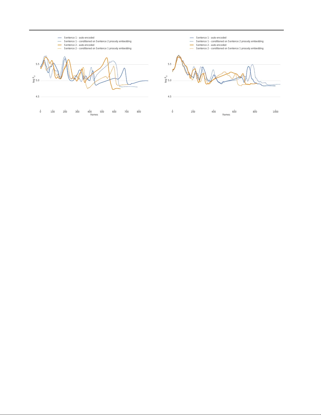
CHiVE: V arying Pr osody in Speech Synthesis with a Linguistically Driv en Dynamic Hierar chical Conditional V ariational Network V incent W an 1 Chun-an Chan 1 T om Kenter 1 Jakub V it 2 Rob Clark 1 Abstract The prosodic aspects of speech signals produced by current te xt-to-speech systems are typically av eraged o ver training material, and as such lack the variety and li veliness found in natural speech. T o a void monotony and a veraged prosody con- tours, it is desirable to ha ve a way of modeling the variation in the prosodic aspects of speech, so audio signals can be synthesized in multiple ways for a gi ven text. W e present a new , hierar- chically structured conditional v ariational auto- encoder to generate prosodic features (fundamen- tal frequency , energy and duration) suitable for use with a vocoder or a generativ e model like W aveNet. At inference time, an embedding repre- senting the prosody of a sentence may be sampled from the v ariational layer to allow for prosodic variation. T o efficiently capture the hierarchical nature of the linguistic input (words, syllables and phones), both the encoder and decoder parts of the auto-encoder are hierarchical, in line with the linguistic structure, with layers being clocked dynamically at the respective rates. W e show in our experiments that our dynamic hierarchical network outperforms a non-hierarchical state-of- the-art baseline, and, additionally , that prosody transfer across sentences is possible by employ- ing the prosody embedding of one sentence to generate the speech signal of another . 1. Introduction Most current text-to-speech ( TTS ) prosody modeling paradigms implicitly assume a one-to-one mapping between text and prosody and fail to recognize the one-to-many na- ture of the task, i.e., there is a large number of w ays in 1 TTS Research, Google UK, London 2 Univ ersity of W est Bo- hemia, w ork carried out whilst at Google. Correspondence to: T om Kenter < tomk enter@google.com > . Pr oceedings of the 36 th International Conference on Machine Learning , Long Beach, California, PMLR 97, 2019. Copyright 2019 by the author(s). Linguistic features Prosodic features Encoder μ σ sentence prosody embedding Decoder sample Predicted prosodic features Figure 1. High-lev el overvie w of the CHiVE model at training time. which a giv en sequence of words can be spoken. This leads to an a veraging effect and as such a lack of variation and variety in generated synthetic speech. This work aims to model prosody in a way that avoids this problem and works tow ards allo wing mechanisms to control the variation in the generated prosody in a linguistically motiv ated way . Prosody prediction in TTS is usually concerned with pro- viding segment durations and fundamental frequency ( F 0 ) contours for the utterance being synthesized. These targets are used to guide unit selection (Fujii et al., 2003), form the input features to a vocoder (Y oshimura et al., 1999), or driv e a W av eNet-like model (Oord et al., 2016). The way in which prosody models are traditionally b uilt has a num- ber of inherent problems. Firstly , as stated above, there is an underlying assumption that there is a unique mapping from a given text or linguistic specification to a prosodic realization. Secondly , duration is modeled independently of F 0 , e.g., (Zen et al., 2016). Lastly , modeling techniques are generally frame- or phone-based and as such, lack the ability to ensure linguistically valid prosodic contours for an utterance as a whole. In this paper we propose a ne w model to e xplicitly address the problems described abov e. W e present a model called a Clockwork Hierarchical V ariational autoEncoder (CHiVE), that produces F 0 and duration and, additionally , c 0 (the 0th cepstrum coefficient) as ener gy , which is a strong prosodic correlate. In our work, these predicted prosodic features are used to dri ve a W aveNet model (Oord et al., 2016) to produce the final speech signal. The CHiVE model is trained as a conditional variational auto-encoder (Kingma & W elling, 2014; Sohn et al., 2015). A high-le v el graphical overvie w is provided in Figure 1. The encoder has both linguistic features (a matrix repre- sented by a blue rectangle) and prosodic features (green CHiVE: V arying Prosody in Speech Synthesis rectangle) as input, and encodes these into an embedding using a v ariational bottleneck layer . The linguistic features represent aspects of the input such as part-of-speech for words, syllable information and phone-le v el information. The prosodic features represent acoustic information about the input, in terms of pitch, duration and energy . The vari- ational layer predicts two vectors, which are interpreted as means and variances (the bro wn and orange vectors in Figure 1 respecti vely), used to parameterize an isotropic Gaussian distrib ution, from which an embedding is sampled. The decoder has linguistic features as input (the same ones the encoder has), and is additionally fed an embedding sam- pled from the variational layer . The sampled embedding, in this way , is designed to encode prosodic aspects of the input sentence. W e refer to it as the sentence pr osody embedding . T o capture the linguistic hierarchy incorporated in the input features – provided at the le vel of words, syllables, phones and frames – both the encoder and the decoder are hierarchi- cal, with dynamically clocked layers following the layers in the linguistic structure of an utterance. A unique feature of the CHiVE mdoel is that the structure of the network is dynamic, i.e., the unrolled recurrent structure of the model is dif ferent for e very input sentence, de pending on the lin- guistic structure of that sentence. The model is described in full in § 3. W e show in our experiments that our dynamic hi- erarchical network outperforms a non-hierarchical baseline. The main value of CHiVE lies in the distribution learned by the v ariational layer , which represents a space of v alid prosodic specifications. At inference time, two dif ferent scenarios can be employed to make use of this space. The first scenario is where we discard the encoder , and choose or sample a sentence prosody embedding from the Gaussian prior , trained at the variational layer . The zero vector can be chosen, which, by design, is the mean of the sentence prosody embedding space, and in our e xperience tends to represent prosody which exhibits the a veraging ef- fect as seen in models such as (Zen et al., 2016). The second scenario is similar to the setup at training time, where a sentence is encoded by the encoder . Y et, instead of trying to reproduce the prosodic features of the input sentence as in the auto-encoder setting during training, we can use the predicted sentence prosody embedding to gen- erate speech for a different sentence, thereby transferring the prosody of one sentence to another . In this setting, the decoder gets the linguistic features of the new sentence as input, while it is conditioned on a sentence prosody embed- ding of a reference sentence. This w ay , the speech for the textual content of the ne w sentence will be synthesized with the prosody of the reference sentence. In short, our contributions are: • W e present CHiVE, a linguistically driv en dynamic hierarchical conditional v ariational auto-encoder , the first of its kind to ha ve a dynamic netw ork layout that depends on the linguistic structure of its input. • W e show that the CHiVE model yields a meaningful prosodic space, by showing that prosodic features sam- pled from it yield synthesized audio superior to the au- dio based on features sampled from a non-hierarchical variational baseline. • W e illustrate prosody transfer , where the prosody of a reference sentence, as captured by the v ariational layer in the CHiVE model, can be used to synthesize speech for another sentence. 2. Related W ork W e discuss work related to three aspects of the CHiVE model we present: modelling of prosody , hierarchcial mod- els and variational models. 2.1. Modeling prosody Early parametric approaches to TTS using hidden Marko v models (HMMs) adopted a “bucket of Gaussians” approach to duration modeling (Y oshimura et al., 1998) which easily fits within the HMM architecture. This could be consid- ered a step backwards from earlier approaches, for example: (Black et al., 1998; V an Santen, 1994; Goubanov a & King, 2008) Additionaly , in these models F 0 is considered as just another acoustic feature, i.e., a local feature of a context- dependent phone, rather than a supra-segmental property of the utterance; earlier work including (Fujisaki & Hirose, 1984; Black & Hunt, 1996; V ainio et al., 1999) was ignored. This trend continued with the mo v e to deep neural netw orks (Zen et al., 2013; Zen & Sak, 2015). There are a fe w excep- tions. In (Mixdorff & Jokisch, 2001) a feed forward neural network is presented to predict prosody using a Fujisaki- style model, but they only apply it to re-synthesis rather than TTS ; In (T okuda et al., 2016), an integrated model is proposed using a hidden semi-Markov model within a neural network framew ork. In contrast to the early work described above work, our approach models the primary acoustic prosodic features used to realize prosody jointly , and across the full sequence. An alternativ e approach to modeling prosody explicitly is taken by end-to-end approaches to TTS , for example, (Ping et al., 2017; W ang et al., 2017) where there is no explicit prosody model at all, and any modeling of prosody is per- formed implicitly within the model. T o a large extent these end-to-end based approaches appear to be able to generate natural prosody and expression, howe ver , in their current forms it is not clear ho w to obtain v aried prosodic patterns. Recent work with style tokens (W ang et al., 2018) attempts to address this point, but the style that can be controlled so far is quite abstract. Style tokens may guide utterance le v el CHiVE: V arying Prosody in Speech Synthesis prosodic features such as emotion, pitch range, or speaking- rate, but the representations learned by the tokens do not necessarily represent clear useful styles. In short, the task style tokens are designed for – capturing a particular style across many utterances – is different from the one we ad- dress here: varying the intonational aspects of prosody per utterance. 2.2. Hierarchical models Hierarchical models are popular in natural language process- ing, e.g., to encode sentence embeddings from the sequence of words in them (Serban et al., 2017; Kenter & de Rijke, 2017), or to construct sentence representation from a se- quence of words, which are in turn treated as sequences of characters, or bytes (Jozefo wicz et al., 2016; K enter et al., 2018). In TTS , hierarchical networks have been explored to a limited extent: (Ronanki et al., 2017) use hierarchical information by ha ving recurrent connections at frame and phone lev els. In other work, (Ribeiro et al., 2016; Y in et al., 2016) try to integrate hierarchical information, but in the context of feed-forward neural networks instead of recurrent neural networks (RNNs). Most similar to our approach are the clockwork models such as (Koutnik et al., 2014), from which we derive the name. Different from that work, the clockwork model we present is run as a conditional variational auto-encoder , rather than as a standard encoder-decoder model. Lastly , (Liu et al., 2015) hav e a set of fix ed clocking speeds that are independent of the input sequence and act within sub-portions of a layer of RNN cells. In contrast to that work, we adopt dynamic clock rates across layers by utilizing sequence-to-sequence encoding techniques. 2.3. V ariational models There are few recent attempts to use V AE-style models in speech synthesis. For example (Akuza wa et al., 2018) pro- pose V AE-Loop where the latent space is used to model expression of speech, and (Henter et al., 2018) use a number of V AE related techniques to sho w that cate gories of acted emotion can be modeled in an unsupervised fashion. (Hsu et al., 2018) present an e xtended T acotron approach combin- ing a variational approach with a basic hierarchical structure to better address separation of latent feature spaces. Again these techniques are concerned with the abstract nature of the utterance prosody such as speaking style rather than being concerned with the details of prosodic meaning. 3. The CHiVE model The CHiVE model learns a mapping between pairs of { x , y } , where x is a sequence of input features, and y a sequence of prosodic parameters. The features describing the linguistic aspects of the input are denoted as x ling uistic . They are provided in a hierarchical fashion – a tree struc- ture – with features at sentence level, word lev el, syllable lev el, phone level and frame lev el. W e denote the features pertaining to the acoustic prosodic information ( F 0 , c 0 and duration) as x prosodic , consisting of x F 0 c 0 and x duration . The prosodic features are presented at multiple le v els as well. Throughout this paper , let p ∈ [0 , . . . , P ] enumerate phones, and t ∈ [0 , . . . , T ] enumerate acoustic frames in sequences x and y . Duration values, x duration p , are pro- vided at phone level, while F 0 and c 0 values, x F 0 c 0 t , are provided at frame le v el. W e note that y = x prosodic , i.e., as the CHiVE model is a (conditional) auto-encoder , its task is to reconstruct the input features x prosodic . Predicting the two output sequences, ˆ y duration and ˆ y F 0 c 0 , is modeled as a regression task. The predictions are computed from the input features by two hierarchical recurrent neural networks (RNNs), with a v ariational layer in between: ˆ µ , ˆ σ = H encoder ( x prosodic , x ling uistic ) ˆ s ∼ N ( ˆ µ , ˆ σ ) ˆ y duration , ˆ y F 0 c 0 = H decoder ( ˆ s , x ling uistic ) . The hierarchical encoder and decoder , and the way they handle features, are described in more detail in § 3.1 and § 3.3, respectively . The sentence prosody embedding ˆ s is sampled from an isotropic multi-dimensional Gaussian dis- tribution, parametrized by predicted mean vector ˆ µ and variance v ector ˆ σ . The network is optimized to minimize two L 2 losses, plus a KL div ergence term for the variational layer: L = λ 1 X p || y duration p − ˆ y duration p || 2 (1) + λ 2 X t || y F 0 c 0 t − ˆ y F 0 c 0 t || 2 + λ 3 D KL [ N ( ˆ µ , ˆ σ ) || N (0 , 1)] , where the first L 2 loss is computed over the durations v alues per phone, the second L 2 loss is computed over the F 0 and c 0 values per frame, and ˆ µ and ˆ σ are the means and variances as predicted by the encoder , respecti vely . The λ terms are used to weight the three losses. The CHiVE model consists of three parts: an encoder , a vari ational layer , and a decoder . W e will describe the design of each of these in turn in this section. Additional details about the hyper-parameters of the netw ork and the features used are discussed in § 4.1.1. 3.1. CHiVE encoder The CHiVE encoder is a hierarchical RNN, composed of three RNNs: a frame-rate RNN and a phone-rate RNN, that both produce syllable-rate output, and a syllable-rate RNN CHiVE: V arying Prosody in Speech Synthesis syllable-rate RNN sample project σ sentence prosody embedding frame-level features sentence-level features syllable-level features word-level features μ frame-rate RNN syllable-rate output phone-level features phone-rate RNN syllable-rate output Figure 2. CHiVE encoder and variational layer . Circles represent blocks of RNN cells, rectangles represent vectors. Broadcasting (vector duplication) is indicated by displaying vectors in a lighter shade of the same colour . (Best vie wed in colour). that takes in the output of the other tw o RNNs, in addition to sentence-, word- and syllable-le vel linguistic input features. Figure 2 giv es a graphical depiction of the CHiVE encoder . The frame-rate RNN, depicted in blue, reads frame-lev el prosodic features ( F 0 and c 0 ), and outputs its internal acti- vation at the end of ev ery syllable. There are usually many frames in a syllable – our e xperiments use a 5 millisecond frame shift – most of which are left out of the figure for clar - ity . The phone-rate RNN runs asynchronously in parallel, and like the frame-rate RNN emits its hidden state at e v ery syllable boundary . In the figure the first syllable consists of two phones and the second syllable of one phone. The states of both LSTMs are reset at syllable boundaries. The outputs of the two RNNs are concatenated and joined with additional syllable-, word- and sentence-level input features. The word-lev el and sentence-le v el input features are broadcast as appropriate, which is indicated in Figure 2 by them having a slightly lighter shade. As we can see from the figure, there is only one sentence-lev el feature vector , broadcast to ev ery time step. Similarly , there are two words, the feature vectors of which are broadcast across their re- spectiv e syllables. Finally , the last hidden activ ation of the syllable-rate RNN is taken to represent the entire input and passed on to a variational layer . The hierarchical layout of the model is designed to reflect the hierarchical nature of the linguistic information that the features represent. W e should note two things concerning the clock rates of the RNNs. Firstly , the number of input feature vectors for the RNN running at frame-rate is differ - ent from the number of input feature v ectors for the one running at phone-rate. Nonetheless both RNNs produce the same number of output v ectors: one for e very syllable. Secondly , the number of input feature vectors at all le v els (frames, phones, syllables and w ords) is dif ferent across sentences. The CHiVE model handles this appropriately , by letting each sub-RNN run at the right clock speed, deter- mined by the number of features provided at that level by the input structure. As such, CHiVE dynamically follo ws the linguistic structure of the input sentence, which is the main feature setting it apart from other models. 3.2. V ariational layer The variational layer takes the last hidden activ ation of the syllable-rate RNN (depicted in dark red in Figure 2) as input, passes it through a fully connected layer , and splits the resulting vector into two vectors, representing the mean and variance of an isotropic multi-v ariate Gaussian (displayed in brown and orange, respectively , in the figure). Finally , a vector is sampled from this Gaussian (displayed in dark yellow), which is used as input to the decoder . 3.3. CHiVE decoder The CHiVE decoder is similar to the encoder , but the hier - archy is re versed. The decoder goes from sentence-le vel to the lev els of syllables, phones and frames. Figure 3 giv es a graphical ov ervie w of the decoder . The sentence prosody embedding output by the variational layer in the previous step (displayed in dark yellow again in the figure) is concatenated with sentence-le vel (yellow), word-le vel (green) and syllable-lev el features (pink), all broadcast as appropriate, and used as input to a syllable-rate RNN that produces one output per syllable. T o reiterate, as we are auto-encoding, the linguistic feature vectors here are the same as those input to the encoder . The next le vel of the decoder is a phone-rate RNN (in pur - CHiVE: V arying Prosody in Speech Synthesis syllable-rate RNN sentence-level features syllable-level features word-level features sentence prosody embedding syllable-level RNN states phoneme-level features phone-rate RNN syllable-level features word-level features sentence-level features phone-level RNN states duration prediction RNN predicted phoneme durations predicted c 0 frame values frame-rate F 0 RNN predicted F 0 frame values 4 + frame-rate c 0 RNN 2 Figure 3. CHiVE decoder . Circles represent blocks of RNN cells, rectangles represent vectors. Broadcasting (vector duplication) is indicated by displaying vectors in a lighter shade of the same colour . (Best viewed in colour). ple), that takes as input each output of the syllable-rate RNN, concatenated with sentence-lev el features, word-le vel fea- tures, syllable-level features (the same ones that fed into the syllable-lev el RNN, simply read again at this stage) and phone-lev el features to produce a sequence of phone repre- sentations. The output acti vations of the phone-rate RNN (in dark purple) are used as input to three different RNNs, that together model the prosodic features, F 0 , c 0 and duration, as highlighted in § 1. Firstly , an RNN predicts phone duration (displayed in or- ange), e xpressed as the number of frames per phone. In Figure 3 the predicted v alues for the first two phones are 2 and 4, respecti vely (these numbers are low to keep the figure clear; in reality these numbers are much higher). Secondly , to predict the c 0 values for each frame, another RNN (in blue) is run for as many steps as predicted by the phone duration RNN, where the corresponding phone-rate RNN output activ ation is repeatedly fed as input at every time step. In the figure, the c 0 RNNs for the first two phones are displayed, which unroll for 2 time steps and 4 time steps for the first and second phone, respectively . The last state of one RNN is used as initial state for the ne xt. In reality , the c 0 RNN is run for every phone b ut for reasons of clarity this is not shown in the figure. Finally , the F 0 values are predicted by another frame-rate RNN (in turquoise), for e very frame in each syllable. T o accomplish this, the durations for all phones in a syllable are summed, and an RNN predicting F 0 val ues is unrolled for as man y steps. So, instead of unrolling this RNN twice – once for 2 steps and once for 4 steps as is the case for the c 0 prediction – the RNN is run once for each syllable, the unroll length of which is the sum of the dura- tions of its constituent phones – 6, for the first syllable in our example in Figure 3. The input at e very time step is the syllable-rate RNN activ ation (dark red), concatenated with the phone-rate RNN activ ation (dark purple) corresponding to the end of the syllable. In Figure 3 this is the second phone, as the first syllable consists of two phones. Again, the F 0 RNN does run for all other syllables too, yet to keep the figure clear , only one frame-le v el F 0 RNN is displayed. W ith respect to the duration values, it should be noted that during training the pr edicted durations are used for calcu- lating the L 2 loss, but the gr ound truth durations are used to determine the unroll lengths of the frame-level c 0 and F 0 RNNs. This allows for easy calculation of the differ- ences between predicted c 0 and F 0 values, which can be computed by a one-to-one matching of frames. At inference time there is no ground truth duration av ailable, and the predicted duration values are used. In addition to the features described abov e, ev ery RNN le vel is provided with a timing signal, using a standard cosine coarse encoding technique (Zen et al., 2013). Different dimensions of coding signal are used for different hierarchy lev els: 64 for words, 4 for syllables and phones, and 3 for frames. These timing vectors can be thought of as being part of the features vectors at e very lev el in the model, and are therefore not explicitly depicted in Figures 2 and 3. 4. Experiments Our main experiment compares the prosodic features sam- pled from the distrib ution yielded by our hier archical v ari- ational model to those sampled from a non-hierarchical baseline model. In addition, we illustrate that CHiVE can be used to transfer the prosody of one sentence to another . Speech samples for the main and additional experi- ments, and for the prosody transfer illustrations described below are av ailable at https://google.github.io/ chive- varying- prosody- icml- 2019/ . 4.1. Sampling prosodic features As described in § 1, the aim of CHiVE is to yield a prosodic space from which suitable features can be sampled, to be used by a generativ e model producing speech audio. W e CHiVE: V arying Prosody in Speech Synthesis T able 1. Side-by-side comparison between CHiVE and a baseline non-hierarchical model. Results are found to be significant, with a normal approximation to a binomial test z-v alue=-5.5, and p- value=3.91 × 10 -8 . Baseline preferred neutral CHiVE preferred 292 (30.7%) 220 (23.2%) 438 (46.1%) compare our dynamic hierarchical variational network to a non-hierarchical v ariational network, where the features generated by both are used to driv e the same generati ve model to produce speech audio. 4 . 1 . 1 . E X P E R I M E N TA L M E T H O D O L O G Y Baseline A non-hierarchical baseline was constructed to mirror the CHiVE model but without the dynamic structure. It was a single multi-layer model running at frame time steps, with broadcasting at different le vels, but no dynamic encoding/decoding. T est set The test set consisted of 100 sentences with 10 prosodically dif ferent renditions having been synthesized for each, both for our hierarchical CHiVE model, and for the non-hierarchical baseline. That is, for each sentence we sampled 10 sentence prosody embeddings from each model and run the associated decoder to produce prosodic features, which we then supplied to Parallel W aveNet (Oord et al., 2017) to produce speech. The W aveNet model made use of the duration and F 0 features, but not c 0 . W e then randomly paired audio samples of the same sentence, one from each model, which gav e us 1000 test sample pairs. W e performed a side-by-side AB comparison, where raters were asked to indicate which of two audio samples of a pair the y thought was better . Each rater receiv ed a random selection of pairs to rate and each pair was rated once. T raining and eval set Our training data was recorded by 22 American English speakers in studio conditions, the number of male and female speakers being balanced. The data consists of 161 000 lines, from a range of domains, including jokes, poems, W ikipedia and other web data. The ev aluation data for hyperparameter tuning was a set of 100 randomly selected sentences per speaker , held out from training. The input features used include information about phoneme identity , number of syllables, dependency parse tree. W e closely followed pre vious work (Zen & Sak, 2015), with two main differences: 1) a one-hot speaker identification feature was added and 2) features are split into lev els corresponding to the le vels of the linguistic structure. Hyperparameters Both the CHiVE prosody model and the non-hierarchical baseline use LSTM cells. The RNNs at each le vel of the hierarchy consist of two LSTM lay- ers. The variational layer predicts the parameters of a 256- T able 2. Results of MOS test comparing CHiVE to the baseline model. The interv al sho wn is 95% confidence around the mean. MOS Baseline based on (Zen et al., 2016) 4.01 ± 0.11 CHiVE - zero embedding 4.07 ± 0.10 CHiVE - encoded embedding 4.25 ± 0.10 Real speech 4.67 ± 0.07 dimensional Gaussian distribution. The hidden layers of the syllable and phone-lev el RNNs ha ve dimension 32 at e very layer , both in case of the the encoder and the decoder . W e use a batch size of 4 for training. 4 . 1 . 2 . R E S U LT S T able 1 lists the results of the side-by-side comparison be- tween our CHiVE model and the non-hierarchical baseline model. The speech generated using the CHiVE prosody model is significantly preferred o ver the speech generated using the baseline prosody model. W e conclude that incor- porating the hierarchical structure of the linguistic input, as done in CHiVE, yields better performance than processing the exact same features in a non-hierarchical fashion. 4.2. Further Evaluation T o further e v aluate CHiVE’ s performance we perform mean opinion score ( MOS ) tests. Additionally , to gain insight into the training phase, we analyse the models in terms of loss. MOS listening tests T o e v aluate the quality of the dif- ferent methods of obtaining sentence le vel embeddings we performed a series of MOS listening tests. W e compare using an all-zero sentence prosody embedding to an embed- ding made by encoding the ground truth audio. As a top-line we include the ground truth audio itself, and as a baseline we include the model from (Zen et al., 2016) as used by W aveNet (Oord et al., 2017) to represent current state of the art. W e choose a test set of 200 expressi v e sentences including jokes, poems and trivia g ame prompts as prosody is an important aspect of their rendition and we want to see how well our model is able to capture this. Raters judge each sentence for naturalness. Results are shown in T able 2 where we see that the zero em- bedding is judged to be slightly , but not significantly , better than the baseline. The encoded version is better still, which is unsurprising as it is using the auto-encoder properties of the model. The performance here is still lower than that of the real speech. This might be caused by the acoustic information being compressed in the v ariational layer, the fact that a sentence prosody embedding is sampled from the encoded distribution or highly expressi v e properties, such as CHiVE: V arying Prosody in Speech Synthesis time Bas eline Encoded Random 1 Random 2 Random 3 Random 4 Random 5 Random 6 Random 7 Random 8 5.5 4.5 6.0 5.0 Natur al speec h Z ero embedding log F 0 Figure 4. A selection of randomly generated log F 0 contours pro- duced by CHiVE for the sentence “That’ s a super choice!”. Con- tours do not align perfectly on the time axis because the predicted phone durations differ per contour . (Best viewed in colour). increased energy or v ocal fry , are still lost by the wa veform generation model as it is currently configured to make use only of the predicted F 0 and duration v alues. W e conclude that while using the zero vector to drive prosody generation yields reasonable natural intonation, it may lack the true expressi veness that the model is capable of generating. W e in vestigate this further below . V ariation of a single utterance Figure 4 shows a range of sampled and reference log F 0 contours for a single sentence. W e first note that the natural speech contour and contour generated by CHiVE in V AE mode, labeled ’Encoded’, are both very similar and e xpressi ve. This shows that the model works well as an encoder-decoder . Secondly we note that the zero-embedding and baseline contours are very similar , and less expressi v e than the natural speech and (auto)encoded speech. This demonstrates the a veraging ef fect of the same text spoken in dif ferent ways—the peaks representing pitch ev ents are broader and less distinct. Finally we see that the randomly sampled sentence prosody embeddings in general produce more expressi v e speech, and produce a wide range of different prosodic patterns, with prominence in dif ferent places. While we hav e not specifically e v aluated the natural- ness of these e xamples, anecdotal e vidence suggests none of them sound unnatural. Perf ormance during training W e present RMSE and absolute error for our hierarchical CHiVE model and the non-hierarchical baseline used in our main experiment, de- scribed in section 4.1.1. The results presented are calculated on a held-out ev aluation set. As noted earlier – when dis- cussing Equation 1, § 3 – the L 2 losses are computed ov er F 0 , c 0 and duration. A breakdown of the overall loss is shown in T able 3. For the line marked ’enc. ’, the sampling step is skipped and the mean values, µ , predicted by the encoder are directly gi ven as input to the decoder . That is, we specifically e valuate both models’ ability to predict suitable durations and F 0 contour giv en the full information of the held-out example being e valuated. From T able 3, we see a 21% relative reduction in the log F 0 RMSE compared to the baseline when the mean v alues pre- T able 3. Loss terms of the non-hierarchical baseline used in main experiment (lines labelled Bsl) and CHiVE, when an embedding sampled from the encoder is used (enc.), a zero embedding (0s), or a random embedding (rnd.). Both absolute error (Abs.) and root mean squared error (RMSE) are sho wn to allo w comparison to other work. log F 0 F 0 c 0 Duration RMSE Abs. (Hz) RMSE RMSE/Abs. (ms) Bsl enc. 0.098 11.18 0.272 0.378 / 0.019 Bsl 0s 0.193 21.52 0.274 0.656 / 0.034 Bsl rnd. 0.238 26.77 0.277 0.715 / 0.037 CHiVE enc. 0.077 8.478 0.287 0.356 / 0.019 CHiVE 0s 0.173 19.16 0.294 0.515 / 0.027 CHiVE rnd. 0.214 24.37 0.298 0.585 / 0.031 dicted by the encoder are used. W e also see that the absolute F 0 loss both when using the zero embedding and random embedding is substantially higher than when the encoded embedding is used. This is expected as these represent ren- ditions of the utterance that are averaged or random, and as such may end up being quite different to the held-out example. The ratio between the F 0 and c 0 in the loss was not tuned, which might e xplain why the distinctive trend in the F 0 seems to be reversed for the c 0 terms, albeit less pronounced. Interestingly , the loss when zero embeddings are used is lower than when random embeddings are used. This is in line with the intuition that zero embeddings represent an av erage, ov erall suitable, prosody , rather than an arbitrary point in the prosodic space. 4.3. Prosody transfer between sentences During training the encoder/decoder portions of the CHiVE model encode/decode the same text and speech. At infer- ence time, howe ver , it is possible to encode one utterance to a sentence prosody embedding and then use that embedding to condition a decoder that generates prosodic features for an entirely different sentence. When CHiVE is run in this fash- ion, the sentence prosody embedding – displayed in dark yellow at the bottom in Figure 3 – represents the prosody of a reference sentence that was input to the encoder , while the sentence-, word-, syllable- and phone-lev el features – displayed in yello w , green, pink and purple respectiv ely – represent another , new sentence, for the decoder to predict the prosodic features for . As a result, the prosody of the ne w sentence is guided by the prosody of the reference sentence. T o illustrate the prosody transfer capabilities of CHiVE, we show log F 0 curves for two pairs of sentences. W e use jokes in our examples, as they hav e a particular prosody pattern, clearly visible in the figures. Note, though, that this is done for illustrati ve purposes only , and that prosody transfer is CHiVE: V arying Prosody in Speech Synthesis 0 100 200 300 400 500 600 700 800 frames 4.5 5.0 5.5 l o g F 0 Sentence 1 - auto-encoded Sentence 1 - conditioned on Sentence 2 prosody embedding Sentence 2 - auto-encoded Sentence 2 - conditioned on Sentence 1 prosody embedding Figure 5. The log F 0 curves for Sentence 1 “What do you call a boomerang that doesn’ t come back? A stic k!” and Sentence 2 “What’ s orang e and sounds like a parr ot? A carr ot. ” conditioned on their o wn sentence prosody embedding (auto-encoded) and each other’ s sentence prosody embedding. not restricted in any way to a particular type of sentence. Figures 5 and 6 both sho w the log F 0 curves of two sen- tences. T wo curves are shown for each sentence: the solid lines are the result of running CHiVE in the auto-encoder setting; the dashed lines are the result of conditioning the decoder for one sentence on the sentence prosody embed- ding of the other . If no prosody transfer would take place, the pair of curv es per sentence – the two blue lines, and the two orange lines in Figures 5 and 6 – would overlap. Howe v er , as can be observed from the figures, the opposite happens, where the dashed lines follow the solid lines of dif ferent colour . In Figure 5, the dashed orange line, instead of closely fol- lowi ng the solid orange line, is guided by the solid blue line as well. It clearly mimmicks the solid blue line near the end, where the punch line is deliv ered. The two curv es do not perfectly ov erlap as there is a mismatch in terms of lengths (in words and syllables), which indicates that, ev en if the two sentences do not perfectly align in terms of syllable structure, meaningful prosody transfer can take place. In Figure 6 we see a similar effect, where at the start, both the solid blue/dashed orange curves and the solid or- ange/dashed blue curves are closely tied. The transfer is not perfect, as can be seen, e.g., near the end, where the two blue line ends up much like each other , without, apparently , follo wing the guidance of the reference prosody embedding, with something similar happening to the orange curves. As these examples illustrate, the variational CHiVE model can be used to transfer prosody from one sentence to another . Additional research is needed for a more rigorous analysis, to see what aspects af fect succes or f ailure of transfer , and if transfer can be extended more generally to, e.g., speaking style. Initial inv estigations with texts containing the same 0 200 400 600 800 1000 frames 4.5 5.0 5.5 l o g F 0 Sentence 1 - auto-encoded Sentence 1 - conditioned on Sentence 2 prosody embedding Sentence 2 - auto-encoded Sentence 2 - conditioned on Sentence 1 prosody embedding Figure 6. The log F 0 curves for Sentence 1 “What do you get when you put a vest on an alligator? An investigator . ” and Sentence 2 “What do you get fr om a pampered cow? Spoiled milk. ” conditioned on their own sentence prosody embedding (auto-encoded) and each other’ s sentence prosody embedding. number of words suggests that specific prosodic patterns transfer between utterances, ev en when the number of sylla- bles per word is dif ferent, and that prominence transfers to the correct syllable in the target sentence. 5. Conclusion Our model, CHiVE, a linguistically dri v en dynamic hierar- chical conditional variational auto-encoder model, meets the objectiv e of yielding a prosodic space from which meaning- ful prosodic features can be sampled to generate a v ariety of valid prosodic contours. W e showed that the prosody gener- ated by the model, when using the mean of the distribution modeled in the v ariational layer (the zero embedding) per- forms as well as current state of the art. W e also sho wed that the hierarchical structure yields speech with a higher variety in natural pitch contours for a gi ven text when compared to a model without this hierarchy . Lastly , we illustrated that the sentence embedding produced by the encoder, that captures the prosody of one utterance, can be used to transfer the prosody to another text. CHiVE can capture natural prosodic variations originally not inferable from the linguistic features it gets as input. This opens opportunities for speech synthesis systems to sound more natural, particularly when synthesizing longer pieces of text – e.g., when a digital assistant reads out a long answer or an entire audiobook – as in these settings repeated use of a default prosody can become tiring to listen to. As the space captured by our hierarchical v ariational model is continuous – arbitrary points yield natural sounding prosody – it would be natural to want to control this space, e.g., by manually selecting a point in it rather than random sampling. Future work will concentrate on making the utter- ance embedding space interpretable in a meaningful way . CHiVE: V arying Prosody in Speech Synthesis Acknowledgments W e would like to acknowledge contrib utions from the Google AI wider TTS research community and DeepMind, calling out specifically contributions from DeepMind in building c 0 conditioned W aveNet Models, and helpful dis- cussion and technical help with ev aluation from the Sound Understanding team. References Akuzawa, K., Iwasawa, Y ., and Matsuo, Y . Expressiv e speech synthesis via modeling expressions with varia- tional autoencoder . In Pr oceedings of Interspeech 2018 , pp. 3067–3071, 2018. Black, A. and Hunt, A. Generating F0 contours from T oBI labels using linear regression. In Proceedings of ICSLP ’96 , volume 3, pp. 1385–1388, 11 1996. ISBN 0-7803- 3555-4. Black, A., T aylor , P ., Caley , R., and Clark, R. The Festiv al speech synthesis system, 1998. Fujii, K., Kashioka, H., and Campbell, N. T arget cost of F0 based on polynomial regression in concatenativ e speech synthesis. In Pr oceedings of the 15th International Congr ess of Phonetic Sciences , pp. 2577–2580, 2003. Fujisaki, H. and Hirose, K. Analysis of v oice fundamental frequency contours for declarati ve sentences of Japanese. Journal of the Acoustical Society of J apan (E) , 5(4):233– 242, 1984. Goubanov a, O. and King, S. Bayesian networks for phone duration prediction. Speech communication , 50(4):301– 311, 2008. Henter , G. E., Lorenzo-T rueba, J., W ang, X., and Y amag- ishi, J. Deep encoder-decoder models for unsupervised learning of controllable speech synthesis. arXiv pr eprint arXiv:1807.11470 , 2018. Hsu, W .-N., Zhang, Y ., W eiss, R. J., Zen, H., W u, Y ., W ang, Y ., Cao, Y ., Jia, Y ., Chen, Z., Shen, J., et al. Hierarchical generativ e modeling for controllable speech synthesis. arXiv pr eprint arXiv:1810.07217 , 2018. Forthcoming at ICLR 2019. Jozefowicz, R., V inyals, O., Schuster , M., Shazeer, N., and W u, Y . Exploring the limits of language modeling. arXiv pr eprint arXiv:1602.02410 , 2016. Kenter , T . and de Rijke, M. Attentiv e memory networks: Efficient machine reading for con versational search. In Pr oceedings of the 1st International W orkshop on Con ver - sational Appr oaches to Information Retrieval (CAIR’17) at the 40th International A CM SIGIR Confer ence on Re- sear c h and Development in Information Retrieval (SIGIR 2017) , 2017. Kenter , T ., Jones, L., and He wlett, D. Byte-level machine reading across morphologically v aried languages. In Pr oceedings of the Thirty-Second AAAI Conference on Artificial Intelligence (AAAI-18) , pp. 5820–5827, 2018. Kingma, D. P . and W elling, M. Auto-encoding v ariational Bayes. In International Confer ence on Learning Repr e- sentations (ICLR) , 2014. K outnik, J., Greff, K., Gomez, F ., and Schmidhuber, J. A clockwork RNN. In International Confer ence on Machine Learning , pp. 1863–1871, 2014. Liu, P ., Qiu, X., Chen, X., W u, S., and Huang, X. Multi- timescale long short-term memory neural network for modelling sentences and documents. In Pr oceedings of the 2015 conference on empirical methods in natural language pr ocessing , pp. 2326–2335, 2015. Mixdorff, H. and Jokisch, O. Building an integrated prosodic model of German. In Seventh Eur opean Confer- ence on Speech Communication and T ec hnology , 2001. Oord, A. v . d., Dieleman, S., Zen, H., Simon yan, K., V inyals, O., Gra ves, A., Kalchbrenner, N., Senior, A., and Kavukcuoglu, K. W av eNet: A generative model for raw audio. arXiv pr eprint , abs/1609.03499, 2016. Oord, A. v . d., Li, Y ., Babuschkin, I., Simonyan, K., V inyals, O., Ka vukcuoglu, K., Driessche, G. v . d., Lock- hart, E., Cobo, L. C., Stimber g, F ., et al. Parallel W aveNet: F ast high-fidelity speech synthesis. arXiv pr eprint , abs/1711.10433, 2017. Ping, W ., Peng, K., Gibiansky , A., Arik, S. ¨ O., Kannan, A., Narang, S., Raiman, J., and Miller , J. Deep Voice 3: 2000-speaker neural text-to-speech. arXiv preprint , abs/1710.07654, 2017. Ribeiro, M. S., W atts, O., and Y amagishi, J. Parallel and cas- caded deep neural networks for te xt-to-speech synthesis. In Pr oceedings of SSW , pp. 107–112, 2016. Ronanki, S., W atts, O., and King, S. A hierarchical encoder - decoder model for statistical parametric speech synthe- sis. In Pr oceedings of Interspeech 2017 , pp. 1133–1137, 2017. Serban, I. V ., Sordoni, A., Lowe, R., Charlin, L., Pineau, J., Courville, A. C., and Bengio, Y . A hierarchical latent variable encoder -decoder model for generating dialogues. In AAAI , pp. 3295–3301, 2017. CHiVE: V arying Prosody in Speech Synthesis Sohn, K., Lee, H., and Y an, X. Learning structured output representation using deep conditional generati ve models. In Advances in Neural Information Pr ocessing Systems 28 , pp. 3483–3491, 2015. T okuda, K., Hashimoto, K., Oura, K., and Nankaku, Y . T emporal modeling in neural network based statistical parametric speech synthesis. In Pr oceedings of ISCA Speech Synthesis W orkshop , pp. 113–118, 2016. V ainio, M., Altosaar, T ., Karjalainen, M., Aulanko, R., and W erner , S. Neural network models for Finnish prosody . In Pr oceedings of ICPhS , pp. 2347–2350, 1999. V an Santen, J. P . Assignment of segmental duration in text- to-speech synthesis. Computer Speech & Languag e , 8(2): 95–128, 1994. W ang, Y ., Skerry-Ryan, R., Stanton, D., W u, Y ., W eiss, R. J., Jaitly , N., Y ang, Z., Xiao, Y ., Chen, Z., Bengio, S., Le, Q., Agiomyrgiannakis, Y ., Clark, R., and Saurous, R. A. T acotron: T owards end-to-end speech synthesis. In Pr oc. Interspeech 2017 , pp. 4006–4010, 2017. W ang, Y ., Stanton, D., Zhang, Y ., Ryan, R.-S., Battenber g, E., Shor , J., Xiao, Y ., Jia, Y ., Ren, F ., and Saurous, R. A. Style tokens: Unsupervised style modeling, control and transfer in e nd-to-end speech synthesis. In Pr oceedings of the 35th International Confer ence on Machine Learning , volume 80 of Proceedings of Mac hine Learning Resear c h , pp. 5180–5189. PMLR, 2018. Y in, X., Lei, M., Qian, Y ., Soong, F . K., He, L., Ling, Z.-H., and Dai, L.-R. Modeling f0 trajectories in hierarchically structured deep neural networks. Speech Communication , 76:82–92, 2016. Y oshimura, T ., T okuda, K., Masuko, T ., K obayashi, T ., and Kitamura, T . Duration modeling for HMM-based speech synthesis. In ICSLP , volume 98, pp. 29–32, 1998. Y oshimura, T ., T okuda, K., Masuko, T ., K obayashi, T ., and Kitamura, T . Simultaneous modeling of spectrum, pitch and duration in HMM-based speech synthesis. In Sixth Eur opean Confer ence on Speech Communication and T echnology , 1999. Zen, H. and Sak, H. Unidirectional long short-term memory recurrent neural network with recurrent output layer for low-latenc y speech synthesis. In Acoustics, Speech and Signal Processing (ICASSP), 2015 IEEE International Confer ence on , pp. 4470–4474. IEEE, 2015. Zen, H., Senior , A., and Schuster , M. Statistical parametric speech synthesis using deep neural networks. In Acous- tics, Speech and Signal Pr ocessing (ICASSP), 2013 IEEE International Confer ence on , pp. 7962–7966. IEEE, 2013. Zen, H., Agiomyrgiannakis, Y ., Egberts, N., Henderson, F ., and Szczepaniak, P . Fast, compact, and high quality LSTM-RNN based statistical parametric speech synthe- sizers for mobile de vices. In Interspeech 2016, 17th Annual Confer ence of the International Speec h Commu- nication Association , pp. 2273–2277, 2016.