Image-based reconstruction for the impact problems by using DPNNs

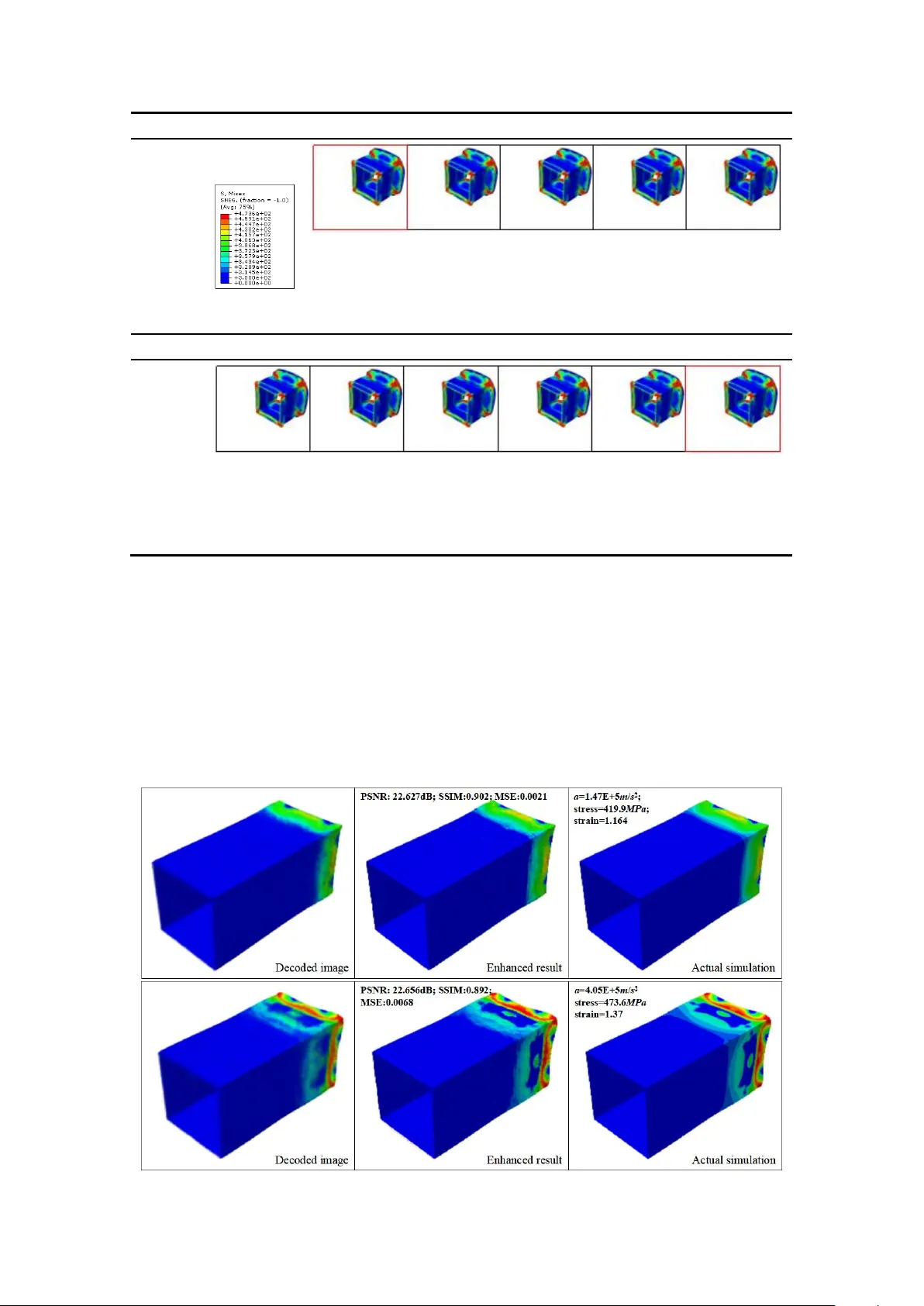
Image-based reconstruction for the impact problems by using DP NN s Y u Li a, * , Hu W ang a, ** , W enquan Shuai a , Honghao Zhang b, c , Y ong Peng b, c a. S tate Key Laboratory of Advanced Design and Manufacturing for V ehicle Body , College of Mechanical and V ehicle Engineering, Hunan University , Changsha, 410082, PR China b. Key Laboratory of T raffic Safety on T rack of Ministry of E ducation, School of T raffic and T ran sportation Engineering, Central South University , Changsha 410000, PR China c. Joint International Resear ch Laboratory of Key T echnology for Rail T raffic Safety , Centr al South University , Changsha, 410000, PR China Abstract W ith the improvement of the pattern recognition and feature extraction of Deep Neural Networks (DPNNs), image-based design and optimization have been widely used in multidisciplinary researches. Recently , a Reconstructive Neural Network (ReConNN) has been proposed to obtain an image-based model from an analysis-based m odel [ 1 , 2 ], and a steady-state heat transfer of a heat sink has been successfully reconstructed. Commonly , this method is suitable to handle stable-state problems. However , it has difficulties handling nonlinear transient impact problems, due to the bottlenecks of the Deep Neural Network ( DPNN ). For example, nonlinear transient problems make it difficult for the Generative Adversarial Network (GAN) to generate various reasonable images. Therefore, in this study , an improved ReConNN method is proposed to address the mentioned weaknesses. T i me-dependent orde red images can be generated. Furt hermore, the improved method is successfully applied in impact simulation c ase and engineering experiment. Through the experiments, comparisons and analys es, the improved method is demonstrated to outperform the former one in terms of its accuracy , efficiency and costs. Keywor ds : EReConNN; Nonlinear transient problem; Impact; Reconstruction; * First author . E-mail addr ess : liyu_hnu@hnu.edu.cn (Y . Li) ** Corresponding author . T el.: +86 0731 88655012; fax: +86 0731 88822051. E-mail: wanghu@hnu.edu.cn (H. W ang) T ime-dependent ordered images. Highlights i. The nonlinear transient impact problem is successfully reconstructed. ii. The adversarial algorit hm is integrated with the V AE and t ermed A V AE. It achieves enhanced performance. iii. The ordered i mages in term of time can be generated based on the manifold learning model. iv. A specific CGAN is suggested for image postprocessing. v. An engineering impact problem of a thin-walled structure is reconstructed well by the EReConNN. Nomenclatur e DP NN Deep Neural Network CNN Convolutional Neural Network ReConNN Reconstructive Neural Network CGAN Conditional GAN EReConNN Enhanced ReConNN MSE Mean Square Error CWGAN Compressed W asserstein GAN KL Kullback – Leibler GAN Generative Adversarial Net work GD Gradient Descent AE Autoencoder JS Jensen-Shannon V AE V ariational AE DOF Degree of Freedom A V AE Adversarial V AE SRGAN Super-Resolution GAN LI Lagrange Interpolation ML Machine Learning DL Deep Learning ESPCN Efficient Sub-Pixel CNN PFHS Plate Fin Heat Sink PSNR Peak Signal- to -Noise Ratio CAD Computer Aided Design SSIM Structural Similarity CIC Convolution in Convolution DRCN Deep Reconstruction-Classification Network SIMP Solid Isotropic Material with Penalization 1. Introduction Currently , with the explosive development of Machine Learning (ML), some ML -based methods, incl uding the Deep Neural Network (DPNN), which is the core technology of Deep Learning (DL), have been utilized in many interdisciplinary studies, such as com putational mechanics [ 3-10 ], heat transfer [ 11 -14 ], fluid mechanics [ 15-18 ], etc. Moreover , with the improvements of the pattern recognition and feature extraction of the DPNNs, increasingly more researchers have attempted to solve some engineering problems based on images . E.g., Lin [ 19 ], Sosnovik [ 20 ], Y u [ 21 ] and Banga [ 22 ] et al used CNN (Convolutional Neural Network) based models to recognize and extract the features of the initial designs of the topologically optim ized designs, and predicted the optimized structure. The testing results based on the Solid Isotropic Material with Penalization (SIMP) method validated that the CNN could significantly reduce the optimization time. For cracks, Fan [ 23 ], Dung [ 24 ] , Dorafshan [ 25 ], Cha [ 26 ], Chen [ 27 ], Y okoyama [ 28 ] and T ong [ 29 ] et al extracted the features of crack images using DPNNs . Through comparisons between the conventional edge detection and the D PNN methods, the DPNNs outpe rformed the conventional methods in crack detection. Additionally , with respect to material studies , Li [ 13 ] stated that the traditional m ethods for studying the effective thermal conductivities of composite m aterials were all based on a good physical understanding, and so he utilized the pattern recognition of the C NN to infer the ef fective thermal conductivities of co mposite materials. Cang [ 30 ] proposed a generative model that created an arbitrary amount of artificial material samples when trained on only a limited amount of authentic samples. The key contribution of this work was the introduction of a morphology constraint to the training of the generative model. For other fields, W ang [ 31 ] proposed a novel full closed-loop approach to detect and classify power quality disturbances based on a deep CNN, and the field data from a multimicro grid system were used to further prove the vali dity of the proposed method. Recently , Reconstructive Neural Network (ReConNN) was proposed as a reconstructive model with the distinctive characteristic framework "from analysis-based models to im age-based m odels". It was developed in R ef. [ 1 ] and further applied to a heat transfer p roblem of a 3D Plate Fin Heat Sink (PFHS) in Ref. [ 2 ]. The R eConNN model was applied to physical field reconstructions and to construct models that included more objective information. However , considering the accuracy , efficiency and cost s, both the ReConNN that proposed in Ref. [ 1 ] and the slightly improved version in Ref. [ 2 ] were in exploratory stages. Some shortcomings in the existing ReConNN are described and analyzed as follows. i. The ReConNN was mainly composed of the CN N and Generative Adversarial Network (GAN). The CNN was e mployed to construct the mapping from the images to the objective functions, while the GAN was utilized to generate more similar images. Nevertheless, because most studies were based on optimization or convergence problems, the CNN might have difficulties constructing high-accuracy mappings from input images to labels 1 , and the GA N does not generate va rious reasonable images. ii. As shown in Fig. 1 (a), the design do main of the PFHS that was previous solved was fixed during the simulation process. This w eak-nonlinear steady-state problem cou ld be handled easily by the ReConNN. However , for nonlinear transient problems, such as the impact problem as shown in Fig. 1 (b), it was powerless. iii. During the ReConNN, a dist inct characteristic of both the CNN and GAN was big data, meaning expensive simulations. However , this study was mainly designed for small samples, and if the necessary dataset was too lar ge, the study would be meaningless. iv. At the end of the work, an interpolation algorithm was needed to complete the reconstruction. Nonetheless, the m atching between the interpolated objective functions and the generated images was inef ficient. time t start t end t i +1 t i t i -1 (a) 3D -PFHS in Ref. [ 2 ] time t start t end t i +1 t i t i -1 1 For NNs, labels denote the real response value of evaluation of samples. (b) Impact problem in this study Fig. 1. Nonlinearity comparisons between different probl ems. T o address the above mentioned shor tcomings, an Enhanced ReConNN (EReConNN) model is proposed. It abandons the previous integrated architecture of the CNN and the GAN. It uses an Adversarial V ariational Autoencoder (A V AE) model to generate the time-dependent ordered images, and avoids the matching work between the generated im ages and corresponding objective functions in the final reconstruction. Through the tests, com parisons and exper iments, the EReConNN outperforms the former one with respect to the accuracy and efficiency , even when nonlinearity exists. The remainder of this study is organized as follows. In Section 2, the basic idea of the impact problem is introduced. Subsequently , Section 3 is devoted to illustrating the structure of the EReConNN. Meanwhile, the generation process of time-dependent ordered images and the reason why the ReConNN is powerless in this study are also described. Then, some detailed numerical examples, results, and analyses are presented in Section 4. In Section 5, the EReConNN reconstructs an actual engineering problem, which is an impact process of a combined multicell thin-walled aluminum structure. Ultimately , some prospective remarks are provided in the final section. 2. Pr oblem descriptio ns 2.1. Physical model The 3D Computer Aided Design (CAD) model of the impact problem is presented in Fig. 2. The impact body is a cuboid whose material is Al alloy 6,061 - T6 , as shown in T able 1. It is defined with an initial velocity v 0 along the negative direction of the z - axis. Furthermore, a 300 kg point mass is coupled in the center of the other side of the impact surface. The total impact tim e is 7 ms . T able 1 The material parameters of the Al alloy 6,061-T6. Parameter V alue Y oung’ s m odulus ( MPa ) 71,275 Poisson’ s ratio 0.33 Y ie ld stress ( MPa ) 241.5 Density ( t / mm 3 ) 2.9× 10 -9 Hardening curve Y ie ld stress ( MPa ) Plastic deformation 241.5 0 263.0 0.0069 278.8 0.0217 318.8 0.0921 346.7 0.1408 374.5 0.1914 388.8 0.2181 423.8 0.2862 464.3 0.3728 473.6 0.4078 y x z v 0 = 25 m / s 2475 × 4 g rids 150 mm 65 mm 65 mm Poin t ma ss Fig. 2. The CAD m odel of th e impact problem. 2.2. Mathematical model In the im pact process, the work is done by the external forces duri ng the deformation. If there is no heat loss , the work will be completely converted into strain energy . UA  (1) The strain energy of the per unit volume is calculated by   00 , , , , , x y z xy yz zx UU        (2) s.t. 1 1 1 ,, xy xy yz yz zx zx G G G          (3) where   21 E G    (4) Here, A is the work done by the external forces; U is the strain energy; ε is the strain; E and v are the Y oung’ s m odulus and the Poisson’ s ratio that defin e the elastic properties, respectively; τ is the shear stress; and G is the shear modulus. The distortion and destruction of the impact body generally contain two stages, el astic deformation and plas tic deformation. When the body is in the elastic- plastic stage, the stress and strain do not yet correspond to each other . The equation of the strain compatibility of a 3-dimensional elastic-plastic is represented as 22 2 22 22 2 22 22 2 22 2 2 2 2 2 2 y xy x y yz z x zx z yz xy x xz y yz xy xz yz xy xz z y x x y z y y z x z z x y z x x y z z x y x y z x y z x y z                                                                                                             (5) The simplest form of linear elasticity is the isotropic case, and the stress-strain relationship is given by 1 / / / 0 0 0 / 1 / / 0 0 0 / / 1 / 0 0 0 = 0 0 0 1 / 0 0 0 0 0 0 1 / 0 0 0 0 0 0 1 / xx yy zz xy xy xz xz yz yz E E E E E E E E E G G G                                                              (6) where σ is the stress. In the plastic stage, the characteristics of the stress and strain are nonlinear and not unique, and the strain-state is related to not only the stress but also the stress change. The plastic constitutive relation can be r epresented as       13 , 22 13 , 22 13 , 22 pp ii x x y z xy x y ii pp ii y y x z yz yz ii pp ii z z x y z x zx ii dd dd dd dd dd dd                                                         (7) It can be further short en ed as the Levy-Mises function. 3 2 p i ij ij i d d    ε S (8) s.t. x m xy xz ij yx y m yz zx zy z m                     S (9) where 1 2 3 m        (10) Here, ε p is the plastic strain increment; and S ij is the deflection stress tensor or stress deviator . 2.3. Implicit algorithm for dynamic pr oblems Dynamic problems are mainly researched with respect to the dynamic response of the structure in basic motions or under dynamic forces. Currently , the Newmark - β method [ 32 ] is one of the most widely used implicit algorithms for dynamical systems with arbitrary excitation. The initial structural equation of the motion for a linear system with dynamic forces is calculated by         0 0 0 0 M r t C r t K r t F t    ( 11 ) where M 0 , C 0 , and K 0 are the initial mass, damping and stiffness matrices, respectively;   rt ,   r t and   rt are the functions of ti me t for the nodal displacement, the nodal velocity and the nodal acceleration, respectively; and F 0 ( t ) is the ini tial load vector of the nodal force with arbitrary excitation. T o compute the initial structural dynamic response using the Newmark- β method , first it needs to determine the M 0 , C 0 , and K 0 . Then, () r t and () rt can be obtained, and the initial nodal acceleration is represented by         1 0 0 0 0 0 0 0 r M F C r t K r       (12) After that, the following related coefficients can be inferred according to time step ∆ t and parameters γ and β. 0 1 2 3 2 1 1 1 , , , 1 , 2 γ a a a a β t β t β t β           4 5 6 7 1 , 1 , 1 , 2 γ γ a a t a t γ a γ t β β              (13) Finally , the effective stif fness matrix 0 K can be presented by 0 0 0 0 1 0 K K a M a C    (14) As for each time step, the ef fective load vector F at t + △ t is                 0 0 0 1 2 0 1 4 5 F t t F t t M a r t a r t a r t C a r t a r t a r t                    (15) The correspondingly nodal displacement r , no dal acceleration r and nodal velocity r are given by Eqs. (16) - (18).     0 0 F t t r t t K     (16)           0 2 3 r t t a r t t r t a r t a r t           (17)         67 r t t r t a r t a r t t        (18) 3. The ar chitectur e of the proposed EReConNN Different from the ReConNN whose main tasks are image regression (Convolution in Convolution, CIC) and image generation (Compressed W asserstein GAN, CWGAN), the EReConNN is mainly composed of feature extraction, physical field reconstruction and visualization enhancement by using the A V AE an d Conditional GAN (CGAN), respectively . As shown in Fig. 3, in Step i, the contour image of each iteration during the simulation is collected. In this study , the mappings on z Oy and x = y = z are chosen as the subjects being investigated. Then the A V AE is employed to extract the features of the physical field in S tep ii. After that, the time-dependent ordered feature values are interpolated in Step iii. Subsequently , all features are decoded by the decoder of the A V AE that is trained in Step ii and the time-dependent ordered images can be generated. The rec onstruction can be completed. Finally , the CGAN is applied to enhance the visualization of the reconstruction. Fig. 3. The architecture of the EReConN N model. 3.1. Bilinear Interpolation The pixel sizes of each simulated image are 480× 960× 3 and 785× 880× 3 when mapping on the surfaces of xOy and x = y = z , respectively . T o improve the univer sality of the algorithm, all images are resized to 256× 256× 3 by using the Bilinear Interpolation before training. In mathematics, the Bilinear Interpolation is an extension of the Linear Interpolation for interpolating the functions of two variables (e.g., x and y ) on a rectilinear 2D grid. The key idea is to perform linear interpolation first in one direction, and then again in another direction. Although each step is linear , the interpolation as a whole is not linear but rather quadratic. If a point ( x , y ) of an unknown function f ( x ) is interpolated through another four points Q ii =( x i , y i ), Q ij =( x i , y j ), Q ji =( x j , y i ) and Q jj =( x j , y j ), the linear interpolation in the x -direction is first done and this yields       , j i i ii ji j i j i xx xx f x y f Q f Q x x x x     (19)       , j i j ij jj j i j i xx xx f x y f Q f Q x x x x     (20) After that, the interpolation in the y -direction is processed to obtain the desired estimate.               1 , ii ij j ji i j i j i ji jj f Q f Q yy f x y x x x x yy x x y y f Q f Q                (21) 3.2. Adversarial V ariational Autoencoder An Autoencoder (AE) [ 33 ] is a feed-forward NN that is trained to approximate the identity function. That is, it is trained to map from a vector of values to the same vector . When it is used for di mensionality reductions, the first half of the network (encoder) is a model that maps from high- dimensional to low-dimensional spaces, and the second half (decoder) maps from low -dimensional to high- dimensional spaces. Compared with the AE, the outputs fro m the encoder in the V AE [ 34 , 35 ] have two purposes: one represents the mean of a Gaussian distribution (z_mean, μ ), and the another represents the logarithmic value of the variance of a Gaussian distribution (z_log_var , log σ 2 ). The i nput to the decoder can be calculated by 2 lo g ex p 2 σ z μ ε       (22) where ε ~ N (0, 1). The optimized objec tive mainly includes two par ts. One is the Mean Squared Error (MSE) that is calculated by Eq. (23). The smaller the MSE is, the more similar the predicted values are to the real samples. The other is the Kullback – Leibler (KL) divergence that is represented by Eq. (24). It constrains z_mean and z_log_var . The optimized objec tive is to minimize the weighted summation of the MSE and the KL divergence, as expressed by Eq. (25).   2 1 ˆ M SE y y n   (23)   2 2 2 2 2 2 1 log 1 log exp log KL               (24) 0.5 0.5 VAE L M SE KL  (25) where y is the training sample; ˆ y is the predicted value; and n is the sample size. In this study , in order to improve the image res toration and feature extr action abilities, the adversarial algorithm is integrated with the V AE as the A V AE, as shown in Fig. 4. Similar to the GAN, a discriminator is added. Th rough judging whether the input is real or fake, the images decoded by the V AE can be further improved. As shown in T able 2, the encoder , decoder and discriminator mainly conta in 6 convolutional or up sampling layers, respectively . A batch norm layer is added to each convolutional layer to normalize the data and improve the training speed, except for the last convolutional laye r in the discriminat or . In the encoder , after the convolutional process, a full connection layer is used to obtain the features with the required dimension. Meanwhile, a dropout layer is employed in the decoder and the discriminator to avoid the overfitting probl em. The loss of the discriminator is calculated by         D L D x D G z       (26) where x is the image from the training samples; and z is a noise vector . ɛ ~ N (0, 1) z_log_ var z_mean + z × r eal fa k e x Decoder Discr imin a t or E n cod er V AE p r ed ict Fig. 4. The architecture of the A V AE. T able 2 The detailed architecture parameters of the A V AE. Layer Kernel size Kernel stride Output deep Encoder Conv-Batchnorm 1 4× 4 2 32 Conv-Batchnorm 2 4× 4 2 32× 2 Conv-Batchnorm 3 4× 4 2 32× 4 Conv-Batchnorm 4 4× 4 2 32× 8 Conv-Batchnorm 5 4× 4 2 32× 16 Conv-Batchnorm 6 4× 4 2 32 Full connection Output nodes = Feature dimension Decoder Full connection Output nodes = 512 Up sampling-Dropout 1 4× 4 2 32× 16 Up sampling-Dropout 2 4× 4 2 32× 8 Up sampling-Dropout 3 4× 4 2 32× 4 Up sampling-Dropout 4 4× 4 2 32× 2 Up sampling-Dropout 5 4× 4 2 32 Up sampling 4× 4 2 3 Discriminator Conv-Batchnorm 1 4× 4 2 32 Conv-Batchnorm 2 4× 4 2 32× 2 Conv-Batchnorm 3 4× 4 2 32× 4 Conv-Batchnorm 4 4× 4 2 32× 8 Conv-Batchnorm 5 4× 4 2 32× 16 Conv-Dropout 4× 4 2 1 3.2.1. The analyses of the pow erless of the CWGAN in the ReConNN. Compared with the EReConNN, th e generative model of the ReConNN is the CWGAN. Meanwhile, through tests, the CWGAN might be powerless for a nonlinear case in this study . The main reasons for the unsatisfactory results are discussed as follows. · First ly , as mentioned by Goodfellow , training GANs requires finding a Nash equilibrium [ 36 ]. However, only when the function is convex can the Gradient Descent (GD) algorithm realize the Nash equilibrium, which means that the GAN has dif ficulties reaching the Nash equilibrium in every training. · The GAN is defined as a min- ma x problem without loss functions, and so it is difficult to determ ine if the direction of the training process is right. · Importantly , compared with other generative models, e.g., A V AE, the GAN uses a Gaussian or uniform distribution to approximate the real data. However , if the input image is too large, too many pixels make the GAN uncontrollable. This is why the images were compressed using a V AE. · Nevertheless, although the compressed images decrease, the input to the GAN is changed from i mage data to discrete data. In the GAN, the output from the generator passes a Softmax layer [ 37 ] using Eq. (27). The Softmax regression changes the input to a probability distribution. Meanwhil e, the final output will be a one -hot matrix. In ML, a one-hot is a group of bits in which the legal combinations of values are only those with a single high (one) bit and all the others low (zero) [ 38 ]. However , the discriminator might give the same judgement for different inputs, which causes the GAN to be unsuitable for learning discrete data . For example, the one -hot matrices of (0.2, 0.3, 0.1, 0.2) and (0.2, 0.25, 0.2, 0.1) are both (0, 1, 0, 0). Furthermore, the Jensen-Shannon (JS) divergence [ 39 ] in Eqs. (28) and (29) is used as the training objective of the GAN, a nd it is also inappropriate for addressing discrete data. Despite the WGAN replac ing the JS divergence with the W assertein dist ance [ 40 ] in Eq. (30), the ability to learn discrete data is still lim ited.   1 yi ii n yi i e softmax y y e     (27)               11 2 2 2 2 P x Q x P x Q x JS P Q KL P x KL Q x               (28) s.t.         l og Px KL P Q P x Qx   (29)       12 12 , , W , i nf xy PP P P x y          (30) where [ y 1 , y 2 , …, y i ] is an input tensor to the Soft max layer; and Γ( P 1 , P 2 ) denotes the collection of all measures with marginals P 1 and P 2 on the first and second factors, respectively . 3.2.2. The analyses of the pow erful of the A V AE in the EReConNN. Essentially , the A V AE is a manifold learning model. There are two main distinguishing features of the manifold learning, one is the nonlinear dimensionality reduction, and the other describes the data characterization. As for the dimensionality reduction, high-dimensional data, meaning data containing more than two or three dimensions, can be dif ficult to in terpret. One approach to simplification is to assume that the data of interest lie on an embedded nonlinear manifold within the lower-dim ensional space. If the manifold has a low enough dimension, the data can be visualized. The data characterization reflects the things that can represent the essential data. Manifold learning “re members” the data by “learning” the data characterization, which is similar to a human brain. These two features can help the A V AE outper form other methods in this study . As shown in Fig. 5, each image is regarded as a data point and each pixel is a dimension. Therefore, an image is an m × n -dimensional point in the Euclidean space. If the manifold has a low enough dimension, the im ages can be distributed in a 1-dimensional space. In addition, if the manifold is learned by the A V AE, the linear relation in the local points of the low-dimensional space is as same as the one in the high-dimensional space. Namely , both have 1 1 2 2 ii x w x w x w x      (31) Thus, through trimming (interpolation) the data in the low -dimensional manifold space, meaningful and reasonable data in the high-dimensional space can be obtained. Fig. 5. The diagrammatic sketch of the manifold learning. By the way , the GAN has dif ficulties inferring a pixel using another pixel, and it can only gener ate all pixels at the same time. In contrast, as for the A V AE, the images in the manifold space are relevant to each other , and so it is possible to generalize new examples using interpolation. Herein, through the inter polation of the extracted features, the new images in the high -dimensional manifold space can be gener ated. Thus, the amount of code and the computational costs can be lar gely saved. 3.2.3. Generation of time-dependent order ed images. As shown in Fig. 6, disordered samples are used to train the A V AE . The A V AE can be regarded as two models: one is feature extr action model that includes the encoder , and the other is the image generation model that includes the decoder . After training, the features of the time-dependent ordered images are extracted using the trained encoder , and it can be seen that ea ch dimension of the features can be distributed in a smooth curve. Then, an int erpolation algorithm is e mployed to obtain more features, and the corresponding time-dependent ordered images can be finally obtained by the trained decoder . F ig. 6. Generation of time-dependent ordered images. 3.3. Conditional Generative Adversa rial Network The disadvantage of small samples for the A V AE is the low accuracy , which makes it necessary to do image postprocessing. Currently , there are many methods to improve imag es’ resolution, such as the Super -Resolution GAN (SRGAN) [ 41 ], the SRCNN [ 42 ], the Deep Reconstruction- Classification Network (DRCN) [ 43 ], th e Efficient Sub-Pixel CNN (ESPCN) [ 44 ], etc. However , these methods may not be suitable for this problem because they aim to reconstruct high-resolution images based on low-resolution images, e.g., the SRGAN increas es the resolution by 4 times. Meanwhile, the purpose of this section is to make the generated images more similar to the actual simulated results without changing resolutions. In this study , the CGAN is employed to enhance the visualization. As shown in Fig. 7, the GAN [ 45 ] is a powerful generative model. It is a method for learning a data distribution P model ( x ) and realizing a m odel to sample from it. The GAN consists of two functions: the generator G ( z ) that maps a sample depending on a random or a Gaussian distribution, and the discriminator D ( x ) that determines if an input belongs to the training data set. G ( z ) and D ( x ) are typically learned jointly by alternate training based on game theory principles. Mathematically , the training process can be described as           ~~ min max , l og l og 1 x P da ta z P z G D V D G D x D G z          ( 32) where x is the image from training sa mples P data ; and z is a noise vector that is sampled from the distribution P z . As shown in Fig. 7, the CGAN [ 46 ] is an extension of GANs where both G ( z ) and D ( x ) receive an additional conditioning variable c , yielding G ( z , c ) and D ( x , c ), respectively . This formulati on allows G ( z ) to generate images that are conditioned on c . c can be based on multiple information, e.g., classification labels [ 47 ], partial data for image restoration [ 48 ] or data from dif ferent modalities [ 46 ]. Mathematically , the optimized objective of the CGAN is           ~~ min max , l og l og 1 x P da ta z P z G D V D G D x c D G z c          (33) Additionally , the specific str ucture of the CGAN in thi s study is shown in Fig. 8. It can be seen that the condition is set as the input to both the generator and the discriminator . As for the generator , it looks like an AE. Firstly , the condition is convoluted, and the convoluted result of each layer will be input to the corresponding upsampling layer . Thus, the generator can generate a fake image based on the condition. The contact layer contacts the two tensors in the deep dir ection of the images, namely , the final dimension of the data. The structure of the discriminator is similar to the convolutional architecture of the generator . z G ( z ) G (z ) D ( x ) D (x) GAN G ( z|c ) z c x c D ( x|c ) D (x) G (z ) CGAN x Fig. 7. The architectures of the GAN and the CGAN. e 1 e 2 e 3 e 4 e 5 e 6 e 7 e 1 e 2 e 3 e 4 e 5 e 6 e 7 G en er a t or Conv olution al lay er Con dition Batc h norm layer Up s amplin g laye r Drop out lay er Fake by ge nerato r Cont act lay er Sigm oid lay er Discr im in a t or Real Fake or Fig. 8. The specific structure of the CGAN used in this study . 4. T ests and an alyses In order to evaluate the performance of the EReConNN, ex periments, comparisons and analyses are presented in this section. T o comprehensively represent the reconstruction, two mappings on the surfaces of xOy and x = y = z are reconstructed, respectively . 4.1. The comparisons b etween A V AE and V AE T o compare the A V AE and V AE, the Peak Signal- to -Noise Ratio (PSNR) [ 49 ] and Structural Similarity (SSIM) [ 50 ] are employed. They are calculated by Eqs. (34) - (35) and Eq. (36), respectively . The PSNR is an engineering term for the ratio between the maximum possible power of a signal and the power of the corrupting noise that af fects the fidelity of it s representation. When given a noise-free m × n monochromic image I and its noisy approximation K , Eq. (23) can be changed to     11 2 00 1 ,, nm ij MS E I i j K i j nm       (34) Then, the PSNR is defined as       2 10 10 10 10 l og 20 l og 10 l og dB M AX PS NR M AX M SE M SE          (35) where MAX is the maximum possible pixel value of the image. Usually , it is 255. As for the SSIM, it is used to measure the similarity between two images. The SSIM is designed to improve traditional m ethods such as the PSNR and MSE. It is a value between 0 and 1, and the larger the SSIM is, the better the image quality . It is calculated by         12 2 2 2 2 12 22 I K IK I K I K μ μ c σ c SSIM μ μ c σ σ c       (36) such that     22 1 1 2 2 , c k L c k L  (37) where μ I and μ K are the average pixels of images I and K , respectivel y; 2 I σ and 2 K σ are the pixel variances of i mages I and K , respectively; σ IK is the covariance of I and K ; c 1 and c 2 stabilize the division with wea k denominators; and L is the dynamic range of the pixel values. L =255, k 1 =0.01 and k 2 =0.03 by default. In this section, a cas e sample that is the same as the one in Section 4.2 with 563 is employed. The feature dimension is set as 1. After 150 training epo chs 2 , the mean values of the predicted results are shown in T able 3. The MSE of the A V AE is reduced by approximately 47% compared with the V AE. For the PSNR and SSIM, the A V AE has remarkable increases. 2 In one epoch, all samples should have been trained once. T able 3 Predicted results by using the A V AE and V AE. Method PSNR SSIM MSE A V AE 21.08dB 89.21% 5.50E-3 V AE 19.93dB 84.64% 1.03E-2 4.2. The r econstruction of the mapping on the xOy surface The mapping on the xOy surface of the 3D impact problem looks like a 2D case. From this mapping surface, the computational ability requirements of the A V AE and the CGAN are relative ly low . 4.2.1. Featur e extraction of the physical field. In thi s section, the dimension of the nonlinear transient case is reduced and its essential features will be extracted. The first and most i mportant iss ue is to ensure suitable dimensions for the features. As shown in Fig. 9, with the convolutional layers, the linear features of the physical field are gradually extracted to map the physical field from high-dimensional to low-dimensional spaces. In this section, the dimensions of the features are set as 4, 64, 256 and 784, and the average V AE losses of the total data set are shown in Fig. 10. Each dimensional case is trained for 844,950 steps, namely , 150 epochs, and the number of simulation iterations is 5,633 3 . It can be seen that when the dimension is less than 256, the loss values are not very different. Although it cannot be simply summarized as the lower the feature dimension, the smaller the V AE loss, at least it is demonstrated that i t might be a good choic e to use a low-dimensional feature. Con v1 Con v2 Con v3 Con v4 Con v5 Con v6 128 × 128 64 × 64 32 × 32 16 × 16 8 × 8 n × 1 Stron g-no nlinea r Line ar fe ature s a =2.013E7 m / s 2 Stress=473.6 MPa Strain=195.195 256 × 256 Fig. 9. The process of the feature extraction by the m anifold learning. 3 Thus, the data set contains 5,633 physical field images (training samples). 0 20 40 60 80 100 120 140 0 400 800 1200 1600 2000 VAE loss Epoch featur e dim ensi on = 4 featur e dim ensi on = 64 featur e dim ensi on = 256 featur e dim ensi on = 784 Fig. 10. The average V AE losses during the training processes for dif ferent feature dimensions for the cube mapping on xOy surface. Meanwhile, after the dim ensionality reduction, the WGAN is used to learn and generate the similar characteristic distributions of the physical field, and then the trained A V AE is applied to de code the n ew features. The physical fields that ar e generated by the CWGAN for the 4 different feature dimensions are shown in Fig. 1 1. No matter what the dimension of the features is, the new physical fields lack convincing details and suffer blurred regions, which make them neit her realistic enough nor do they have suf ficiently high resolution. (a) Feature dimension = 4 (b) Feature dimension = 64 (c) Feature dimension = 256 (d) Feature dimension = 784 Fig. 1 1. Generate d results by using the CWGAN in the ReConNN. Actually , the physical quantities affecting the acceleration, stress, strain and other characteristics during the impact are all time related. Accordingly , the DOF of the nonlinear transient impact process is regarded as one, which is the time. Therefore, the dimension of the features is set to 1, and different numbers of it eration steps of the simulation of 281, 563, 1,126, 2,817 and 5,633 are run 4 , respectively . The aver age V AE loss es duri ng the training process are shown in Fig. 12 . Because this study mainly focuses on those engineering probl ems wit h sparser data or expensive computations/simulations, the lower the number of necessary training samples, the more meaningful the study . As shown in Fig. 12, it can be seen that the dif ference of the V AE loss es between using 281 iterations and 5,633 iterations is approximately 4,000. Considering the 20-fold gap in the samples, the difference of 4,000 might be acceptable. T o further visualize the training results of the A V AE by using different samples, the decoded physical fields for several impact times are represented in T able 4. Luckily , no matter what the number of total iterations of the simulation is, the A V AE can decode features well and restore the overall structure. T o better observe and compare different results, enlarged images in the 4 ms are presented in T able 5. W ith the increase of the sample size, the decoded images are more similar to the actual 4 In this way , 28 1, 563, 1,126, 2,817 and 5,633 training samples can be obtained, respectively . simulation results. However , as for the results that are simulated using only 281 iterations, due to the limited sample size, the decoded image is very vague and lacks convincing deta ils, especially in th e areas that are marked by rectangles. For the results from the 5,633 iterations, the 20- fold higher number of simulation iterations truly improves the decoded results. Nevertheless, the images are still vague. Though the detailed features have been improved, ther e is still room for improvement. Therefore, no matter what the number of simulation iterations is, follow-up image enhancement work is necessary and this will be detailedly introduced in the foll owing Section 4.2.3. 0 20 40 60 80 100 120 140 0 4000 8000 12000 16000 20000 VAE loss Epoch Sim u lati on i teration s are 281 Sim u lati on i teration s are 563 Sim u lati on i teration s are 1,126 Sim u lati on i teration s are 2,817 Sim u lati on i teration s are 5,633 Fig. 12. The average V AE losses during training process when simulating dif ferent iterations for the cube mapping on xOy surface. T able 4 The decoded physical fields when simulating different iterations for the cube mapping on xOy surface. where the units of the a and stress are m / s 2 and MPa , respectively . T ime Results 281 iterations 563 iterations 1,126 iterations 2,817 iterations 5,633 iterations 0.01 ms a =0 stress=0 strain=0 0.15 ms a =3.5E+5 stress=1.2E-4 strain=1.157 0.50 ms a =2.6E+6 stress=473.6 strain=1.840 1.80 ms a =7.0E+5 stress=473.6 strain=2.514 4.00 ms a =1.2E+7 stress=473.6 strain=23.10 T able 5 Enlarged images in the 4 ms when simulating different iteratio ns for the cube mapping on xOy surface. Actual simulation 281 iterations 563 iterations 1,126 iterations 2,817 iterations 5,633 iterations In the following ste p, the time-dependent ordered feature values of those cases whose feature dimension is 1 are draw n in the xOy coordinate, as shown in Fig. 13. Interestingly , whatever the number of simulation iterations is, the extracted features of each case can be well distributed on a smooth curve, which can further il lustrate th e manifold learni ng of the A V AE. Thus, the A V AE can well extract the features of the physical field with few simulation iterations. In summary , to easy observe the distribution of the extracted features, and in order to conduct more convenient subsequent feature int erpolation, the dimension of each feature is set as 1. Moreover , by comprehensively considering the visual effect and focusing on problems with few simulation iterations, the simulation with 563 iterations, namely , 563 samples, is selected for follow -up studies. By the way , compared with the 22,000 samples in Ref. [ 1 ] and the 6,055 samples in Ref. [ 2 ], the necessary sample size of 563 is signifi cantly smaller , which makes this study more meaningful. Fig. 13. The features of the physical field in the 1-dimensional manifold space for the cube mapping on xOy surface. 4.2.2. Reconstruction of the physical field. In the ReConNN, after constructing the mapping from the images to the objective functions using the CIC and generating sufficient physical field images using the CWGAN, the curve of the objective functions from the simulation is interpolated. Then, the new objective functions need to be ma nually matched with the generated im ages. Hence, new images can be interpolated into the initial simulations. However , as mentioned in Section 1, the interpolation mode of the R eConNN has some shortcomings. Moreover , it is impossible to guarantee that all structures of the generated physical field images are scientific and reasonable, and so many computational resources are consumed to generate meaningless images, and distinguishing available images from unavailable ones is also inefficient. Finally , the ma tching work between the interpolated objective functions and the new physical field images is time-consuming and laborious. Similar to the ReConNN, the Lagrange Interpolation (LI) is also employed in the EReConNN. However , the LI is no longer applied to the objective functions but is applied to the time-dependent ordered 1-dimensional features of the physical field. Meanwhile, the generative model is also no longer the GAN but is now the decoder of the A V AE. While training the A V AE, the feature extraction model and generative model are trained simultaneously . Th e LI can be expressed by     1 , 1 , 2 , , n ii i f x y p x i n    (38) s.t.               12 1, 1 1 + 1 n n i i i i j ji j j j j j j n x x x x x x xx p xx x x x x x x x x              (39) In this study , the interval of interpolation between adjacent impact it erations is 0.1. Namely , each adjacent iteration will be interpolated by 9 new values. The par tial reconstructed results are shown in T able 6, where I i represents the i -th ( i =1, 2, …, 563) iteration that is run by the simulation, D j ( j =1, 2, …, 9) is the j -th interpolated step, S represents the stress whose actual number of simulation iterations is set as 5,067 (=563× 9), D-S is the interpolated results of the stress between I i and I i+ 1 , and Error is the error of S and D-S. Furthermore, the parts marked with red are the actual iterations that are run by simulation, while others are the interpolated results. T wo iteration processes during the impact are selected to be shown: the first (from I 7 to I 8 ) is the period of violent impact, and the other (from I 324 to I 325 ) gradually converges. It can be inferred that through the decoder of the A V AE, the interpolated features are well decoded and orderly , and it is easy to guarantee that the interpolated objective functions and generated images match well. Moreover , the errors between the interpolated and actual simulation results are less than 10 -4 , which is sufficiently satisfactory . T able 6 The reconstruction of the nonlinear physical field of the impact problem for the cube mapping on xOy surface. Legend I 7 D 1 D 2 D 3 D 4 Image Feature -7.410 -7.379 -7.348 -7.317 -7.2 87 S 404.614 404.972 405.318 405.650 405.964 D-S -- 404.959 405.279 405.580 405.864 Error -- 0.00% 0.01% 0.02% 0.02% D 5 D 6 D 7 D 8 D 9 I 8 Image Feature -7.257 -7.229 -7.201 -7.174 -7.149 -7.125 S 406.256 406.536 406.797 407.037 407.261 407.474 D-S 406.137 406.403 406.665 406.928 407.196 -- Error 0.03% 0.03% 0.03% 0.03% 0.02% -- Legend I 324 D 1 D 2 D 3 D 4 Image Feature 3.924 3.926 3.929 3.931 3.934 S 473.602 473.603 473.605 473.608 473.61 1 D-S -- 473.603 473.605 473.608 473.61 1 Error -- 0.00% 0.00% 0.00% 0.00% D 5 D 6 D 7 D 8 D 9 I 325 Image Feature 3.936 3.939 3.941 3.944 3.946 3.949 S 473.615 473.619 473.622 473.625 473.627 473.627 D-S 473.615 473.619 473.622 473.625 473.627 -- Error 0.00% 0.00% 0.00% 0.00% 0.00% -- 4.2.3. V isualization Enhancement of the physical field. As mentioned before, the reconstructed results lack some detailed features. Therefore, it is necessary to enhance the visualization. The decoded images are used as the inputs to the CGAN while the corresponding simulated images are the learning objectives. The enhanced results are shown in Fig. 14. For the PSNR and SSIM, empirically , if the PSNR and SSIM are larger than 20 dB and 0.9, respectively , the results are acceptable. It can be seen that the CGAN satisfactorily improves the decoded images, especially in those marked areas, and the representation of the detailed features is also greatly improved. Fig. 14. Enhanced results of the reconstruction for the cube mapping on xOy surface. 4.3. The r econstruction of the mapping on the x = y = z surface In this section, the impact mapping on the x = y = z surface is constructed. From this surface, the 3D changes and folding of the body duri ng the impact can be better observed. 4.3.1. Featur e extraction of the physical field. Firstly , the A V AE is applied to extract the physical field features. As mentioned in Section 4.2.1, the final number of si mulation iterations is set as 563, and so the sample size is 563. As shown in Fig. 15, after 150 training epochs, the images that are decided by the A V AE can represent the overall characteristic of the physical field. Furthermore, as shown in Fig. 16, through manifold learning, the physical field is well mapped from high-dimensional to 1-dimensional spaces. Fig. 15. The feature extraction process of the physical field by using the A V AE for the cube mapping on x=y=z surface. Fig. 16. The m anifold distribution of the physical field in 1-dimensional space for the cube mapping on x=y=z surface. 4.3.2. Reconstruction of the physical field. Identical to the reconstruction of the mapping on the xOy surface, the reconstructions from the 7 th to 8 th iterations and from the 324 th to 325 th iterations are shown in T able 7, respectively . Compared with the simulation process, the number o f simulation iterations of the physical field easily increases by 9 times, and the added steps have high enough resolutions and many suf ficiently detailed features. T able 7 The reconstruction of the nonlinear physical field of the impact problem for the cube mapping on x=y=z surface. Legend I 7 D 1 D 2 D 3 D 4 Image Feature -7.410 -7.379 -7.348 -7.317 -7.287 S 404.614 404.972 405.318 405.650 405.964 D-S -- 404.959 405.279 405.580 405.864 Error -- 0.00% 0.01% 0.02% 0.02% D 5 D 6 D 7 D 8 D 9 I 8 Image Feature -7.257 -7.229 -7.201 -7.174 -7.149 -7.125 S 406.256 406.536 406.797 407.037 407.261 407.474 D-S 406.137 406.403 406.665 406.928 407.196 -- Error 0.03% 0.03% 0.03% 0.03% 0.02% -- Legend I 324 D 1 D 2 D 3 D 4 Image Feature 3.924 3.926 3.929 3.931 3.934 S 473.602 473.603 473.605 473.608 473.61 1 D-S -- 473.603 473.605 473.608 473.61 1 Error -- 0.00% 0.00% 0.00% 0.00% D 5 D 6 D 7 D 8 D 9 I 325 Image Feature 3.936 3.939 3.941 3.944 3.946 3.949 S 473.615 473.619 473.622 473.625 473.627 473.627 D-S 473.615 473.619 473.622 473.625 473.627 -- Error 0.00% 0.00% 0.00% 0.00% 0.00% -- 4.3.3. V isualization enhancement of the physical field. The enhanced results after 150 training epochs are shown in Fig. 17. Compared with the mapping on xOy surface, the PSNR and SSIM are slightly worse due to containing more detailed feature s, while the folding is better . Comprehensively , the enhanced results are satisfactory and acceptable. Fig. 17. Enhanced results of the reconstruction for the cube mapping on x=y=z surface. 5. Experiment After the simulated cases, an experiment is necessary to validate the feasibility of the proposed EReConNN for engineering problems. Therefore, an impact experiment is reconstructed. Recently , the structural impacts of vehicles have attracted increasingly attention. A thin- walled metal structure is considered as a promising energy absorber due to its ef ficient energy absorption performance. In this section, the impact of a combined five-cell thin-walled structure that is used in a high speed train [ 51 ] is employed and simulated. Then, the impact process is reconstructed by using limited numbers of simulation iterations. Consequently , a full scale impact experiment is done to validate the reconstructed results. 5.1. Physical model 5.1.1. Combined five-cell structur e. As shown in Fig. 18, the combined multicell thin -walled aluminum structure is installed in the front end of cer tain high speed trains. The units in Fig. 18 are in mm , and the thickness is set as 5 mm . Th e material structure uses Al alloy 6 ,008, as shown in T able 8. It contains one octagonal and four hexagonal tubes. T able 8 The material parameters of the Al alloy 6,008. Parameter V alue Y oung’ s m odulus ( MPa ) 72,000 Poisson’ s rati o 0.33 Y ie ld stress ( MPa ) 131.82 Density ( t / mm 3 ) 2.7× 10 -9 Hardening curve Y ie ld stress ( MPa ) Plastic deformation 131.8 0 140.0 0.0023 149.4 0.0067 162.3 0.0153 171.2 0.0232 178.3 0.0314 183.7 0.0406 187.4 0.0503 189.8 0.0601 190.6 0.0648 191.0 0.0658 56 56 51 410 410 370 20 30 30 50 130 270 F r o n t view Sid e vie w T op view Ene rg y- abso rbin g tub es Indu ced hole Fig. 18. The CAD model of the combined five-cell. 5.1.2. The simulation model of the impact. As shown in Fig. 19, the impact model is composed of an impact trolley , an energy-absorbing structure and rigid tracks. T o remain consistent with actual conditions, 9.81 m / s 2 gravity acceleration is adopted for the entire system. The frictional coef ficients for the static and dynamic conditions are designed as 0.3 and 0.1, respectively . The 2,000 kg trolley collides at an initial velocity of 15.5 10 m / s . Mass points v 0 =15.510 m / s g =9.8 1 m / s 2 Energy-abs orbing structu re Track T est trolle y Fig. 19. The FE m odel and simulation conditions. 5.2. Reconstruction by using the EReConNN In this section, the impact process mapping on the top view is reconstructed, and 100 iterations are simulated to obtain training samples. 5.2.1. Featur e extraction of the physical field. The manifold distribution of the physical field in a 1 -dimensional space is represented in Figs. 20. It can be found that the A V AE well maps the physical field of the combined five-cell structure from high-dimensional to 1-dimensional manifold spaces. Fig. 20. The m anifold distribution in 1-dimensional space for the combined five-cell. 5.2.2. Reconstruction of the physical field. The impact process takes 40 ms , and the impact images at 0 ms , 0.4 ms , 0.8 ms , …, 40 ms in simulation are saved. Namely , the images are sampled at 2,500 frames per second. As shown in T able 9, similar to the reconstruction in Section 4 and taking 0.04 ms as the interpolation step, 9 times the number of iterations of the initial simulation is obtained, namely , the images are sampled at 25,000 frames per second. Furthermore, an experiment is done to evaluate the reconstruction results. The impact process of the experiment is captured by a high speed camera with a frequency o f 5,000 frames per second. It can be seen that the reconstructed impact process is consistent with the experiment. The tubes buckle symmetrically along the central axis. Moreover , a 5 times (if necessary , more times is feasible) greater sampling frequency is adequately used compared with the high speed cam era, which can help us to effectively reduce the computational and equipment costs. T able 9 Comparisons of impact series between reconstructed and experimental. T ime Reconstruction (25,000 frame/ s ) Experiment (5,000 frame/ s ) 0.6 ms 8.2 ms 16.2 ms 24.2 ms 32.2 ms 40.2 ms Conclusions In this study , an EReConNN is developed to solve a nonlinear transient impact case. Simultaneously , the EReConNN addresses some shortcomings of the existing ReConNN. The contrib utions of this study can be summarized as follows. i. The proposed EReConNN is successfully applied to the nonlinear transient case of an impact problem. ii. The adversarial algorithm integrated with V AE and an A V AE is proposed. iii. The integrated m ode of the CNN and GAN is replaced by the proposed A V AE, which completes the feature extraction and time-dependent ordered image generation simultaneously . iv. After reconstruction, the CGAN is innovatively employed to perform the image postprocessing. This makes the rec onstructive results more meaningful and reasonable. v. Finally , an engineering probl em is reconstructed and experimented. The results present that the proposed EReConNN can effectively reduce the computational and equipment costs. Acknowledgments Th is work has been supported by Project of t he Key Program of National Natural Science Foundation of China under the Grant Numbers 1 1572120 and 51621004, Key Projects of the Research Foundation of Education Bureau of Hunan Province (17A224). Refer ence [1]. Li Y , W ang H, Mo K, Zeng T . Reconstruction of Simulation-Based Physical Field by Reconstruction Neural Netw ork Method. 2018;arXiv preprint arXiv: 181 1.02102. [2]. Li Y , W ang H, Deng X. Image-based reconstruction for a 3D-PFHS heat transfer problem by ReConNN. International Jour nal of Heat and Mass T ra nsfer . 2019;1 34:656-67. [3]. Oishi A, Y agawa G . Computational mechanics enhanced by deep learning. Computer Methods in Applied Mechanics and Engi neering. 2017;327:327-51. [4]. Cheng Z, W a ng H. How to control the crack to propagate along the specified path feasibly? Computer Methods in Applied Mechanics and Engineering. 2018; 336:554-77. [5]. Papadopoulos V , Soimiris G , Giovanis DG , Papadrakakis M. A neural network -based surrogate model for carbon nanotubes with geometric nonlinearities. Computer Methods in Applied Mechanics and Engineering. 2018;32 8:41 1-30. [6]. W ang H, Li GY , Li E. Tim e-based metamodeling technique for vehicle crashworthiness optimization. Computer Methods i n Applie d Mechanics & Engineering. 2010;199(37):2497-50 9. [7]. White DA, Arrighi WJ, Kudo J, W atts SE. Multiscale topology optimization using neural network surrogate models. Com puter Methods in Applie d Mechanics and Engineering. 2018. [8]. Lin C-Y , Lin S-H. Artificial neural network based hole image interpretation techniques for integrated topology and shape optimiz ation. Computer methods in applied mechanics and engineering. 2005;194(36-38):3817-37. [9]. Liu Z, W u C. Exploring the 3D architectures of deep material network in data-driven multiscale mechanics. Journal of the Mec hanics and Physics of Solids. 2019. [10]. T yuly ukovskiy E, Huber N. Neural networks for tip correction of spherical indentation curves from bulk metals and thin metal films. Journal of the Mechanics and Physics of Solids. 2007;55(2):391-418. [1 1]. Sheikholeslami M, Gerdroodbary MB, Moradi R, Shafee A, Li Z. Application of Neural Network for estimation of heat transfer treatment of Al2O3-H2O nanofluid through a channel. Computer Methods in Applied Mechanics and Engineering. 2019;344:1-12. [12]. Czé l B, W oodbury KA, Gró f G . Inverse identification of temperature-dependent volumetric heat capacity by neural networks . International Journal of Thermophysics. 2013;34(2):2 84-305. [13]. Li X, Liu Z, Cui S, Luo C, Li C, Zhuang Z. Predicting the effective mechanical prop erty of heterogeneous materials by image based modeling and deep learning. Computer Methods in Applied Mechanics and Engineering. 2019. [14]. Ootao Y KR, T anigawa Y , et al. Optimization of material composition of nonhomogeneous hollow sphere for therm al stress relaxation m aking use of neural network. C omputer m ethods i n a pplied mechanics and engineering. 1999;1 80(1-2): 185-201. [15]. W u J-L, Sun R, Laizet S, Xiao H. Representation of stress tensor pert urbations with application in machine-learning-assisted turbulence modeling. Computer Methods in Applied Mechanics and Engineering. 2019;346:707- 26. [16]. Kuan Y , Lien H, editors . The integration of the neural network and computational fluid dynamics for the heatsink design. Inter national Symposium on Neural Networks; 2005: Springer . [17]. Qi Y , Lu J, Scardovelli R, Zaleski S, T ryggvason G . Com puting curvature for volume of fluid methods using machine lear ning. Journal of Computational Physics. 20 19;377:155-61. [18]. Poloni C, Giur gevich A, On esti L, Pediroda V . Hybridization of a multi- objective genetic algorithm, a neural network and a classical optimizer for a complex design problem in fluid dynamics. Computer Methods in Applied Mechanics & Engineering. 2000;18 6(2):403-20. [19]. Lin Q, Hong J, Liu Z, Li B, W ang J. Investigati on into the topology optimization for conductive heat transfer based on deep learning approach. International Communications in Heat and Mass T ransfer . 2018;97:103- 9. [20]. Sosnovik I, Oseledets I, Sosnovik I, Oseledets I. Neural networks for topology optimization. 2017. [21]. Y u Y , Hur T , Jung J, Jang IG . Deep learning for determining a near-optim al topologi cal design without any iteration. S tructural and Multidisci plinary Optimization. 2018:1-13. [22]. Banga S, Gehani H, Bhilare S, Patel S, Kara L. 3D T opology Optimization using Convolutional Neural Networks. arXiv prepr int arXiv:180807440. 2018. [23]. Fan Z, W u Y , Lu J, Li W . Automatic pavement crack detecti on based on structured prediction with the convolutional neural net work. arXiv preprint arXiv:18020220 8. 2018. [24]. Dung CV . Autonomous concrete crack detection using deep fully convolutional neural network. Automation in Constructio n. 2019;99:52- 8. [25]. Dorafshan S, Thomas RJ, Maguire M. Comparison of deep convolutional neural networks and edge detectors for image-based crack detect ion in concrete. C onstruction and Buildi ng Materials. 2018;186:1031-45. [26]. Cha YJ, Choi W , B ü y ü kö zt ü rk O. Deep learning ‐ based crack damage detection using convolutional neural networks. Computer ‐ Aided Civil and Infrastructure Engineering. 2017;32(5):361-78. [27]. Chen F-C, Jahanshahi MR. NB- CNN: deep learning-based crack detection using c onvolutional neural network and Naï ve Bayes data fusion. IEEE Transactions on Industrial Electronics. 2018;65(5):4392-400. [28]. Y okoyama S, Matsumoto T . Developm ent of an automatic detector of cracks in concrete us ing machine learning. Procedia engi neering. 2017;171:1250- 5. [29]. T ong Z, Gao J, Zhang H. Recognition, location, measurement, and 3D reconstruction of concealed cracks using convolutional ne ural networks. Construction and Buildi ng Materials. 2017;146:775-87. [30]. Cang R, Li H, Y ao H, Jiao Y , Ren Y . Improving direct physical properties prediction of heterogeneous materials from imaging data via convolutional neural network and a morphology-aware generative model. Com putational Materials Science. 2018;150:212-21. [31]. W ang S CH. A novel deep learning method for the classification of power quality disturbances using deep convolutional ne ural network[J]. Applied energy . 2019;235: 1 126-1 140. [32]. Newmark NM. A method of computation for structural dynamics. American Society of Civil Engineers. 1959. [33]. Bengio Y MM, Larochelle H. Nonlocal Estimation of Manifold Structure. Neural Computation. 2006;18(10): 2509-2528. [34]. Kingma DP , W elling M. Auto-enc oding variational bayes. arXiv pre print arXiv:131261 14. 2013. [35]. Doersch C. T utorial on variational autoencoders. ar Xiv preprint arXiv:160605908. 2016. [36].Osborne MJR, Ariel A Course in Game Theory . Cambridge, MA: MIT p 14 ISBN 97 80262 150415 . 12 Jul 1994. [37]. Bishop CM. Pattern Recognition and Mac hine Learning. Springer . 2006. [38]. Harris DaH, Sarah. Digital design and computer architecture. San Francisco, C alif: Morgan Kaufmann. 2010;p. 129. ISBN 978-0- 12 -394424- 5. [39]. Manning HSCD. Foundations of Statistical Natural Language Processing. Cambridge, Mass: MIT Press. 1999;p. 304. ISBN 9 78-0- 262 -13360- 9. [40]. Arjovsky M, Chintala S, Bottou L. W asserstein gan. arXiv preprint arXiv: 170107875. 2017. [41]. Ledig C, Theis L, Huszá r F , Caballero J, Cunningham A, Acosta A, et al., editors. Photo -realistic single image super-resol ution using a generative adversarial network. Proceedings of the IEEE conference on computer vision a nd pattern recognition; 2017. [42]. Dong C, Loy CC, He K, T ang X. Image super-resolution using deep convolutional networks. IEEE transactions on patter n analysis and machine intelligence. 2016;38 (2):295-307. [43]. Ghifary M, Kleijn WB, Zhang M, Balduzzi D, Li W , editors. Deep reconstruction-classification networks for unsupervised do main adaptation. European Conference on Computer V ision; 2016: Springer . [44]. Shi W , Caballero J, Huszá r F , T otz J, Aitken AP , Bishop R, et al., editors. Real-time single image and video super-resolution using an ef ficient sub-pixel convolutional neural network. Proceedings of the IEEE conference on com puter vision and pattern recogn ition; 2016. [45]. Goodfellow IJ, Pouget-Abadie J, Mirza M, Xu B, W arde-Farley D, Ozair S, et al., edit ors. Generative adversarial nets. International Conference on Neural Information Processing Systems; 2014. [46]. Mirza M, Osindero S. Conditional Generative Adversarial Nets. Computer Science. 2014:2672-80. [47]. Denton E L CS, Fer gus R. . Deep Generative Image Models using a Laplacian P yramid of Adversarial Networks. Advances in neural inform ation processing systems. 2015;2015: 1486-1494. [48]. Goodfellow I, Mirza, M., Courville, A., and Bengio, Y . Multi -prediction deep boltzmann machines. Advances in Neural Information Processing Syst ems. 2013;pages 548 – 556. [49]. W elstead ST . Fractal and wavelet image compression techniques: SPIE Op tical Engineering Press Bellingham, W ashington; 1999. [50]. W ang Z, Bovik AC, Sheikh HR, Simoncelli EP . Image quality assessment: from error visibility to structural similarity . I EEE transactions on im age processing. 2004;13(4):600-12. [51]. W ang S, Peng Y , W ang T , Che Q, Xu P . Collision performance and multi-objective robust optimization of a combined multi-cell thin-walled structure for high speed train. Thin-W alled Structures . 2019;135:341-55.