End-to-End Multi-Channel Speech Separation

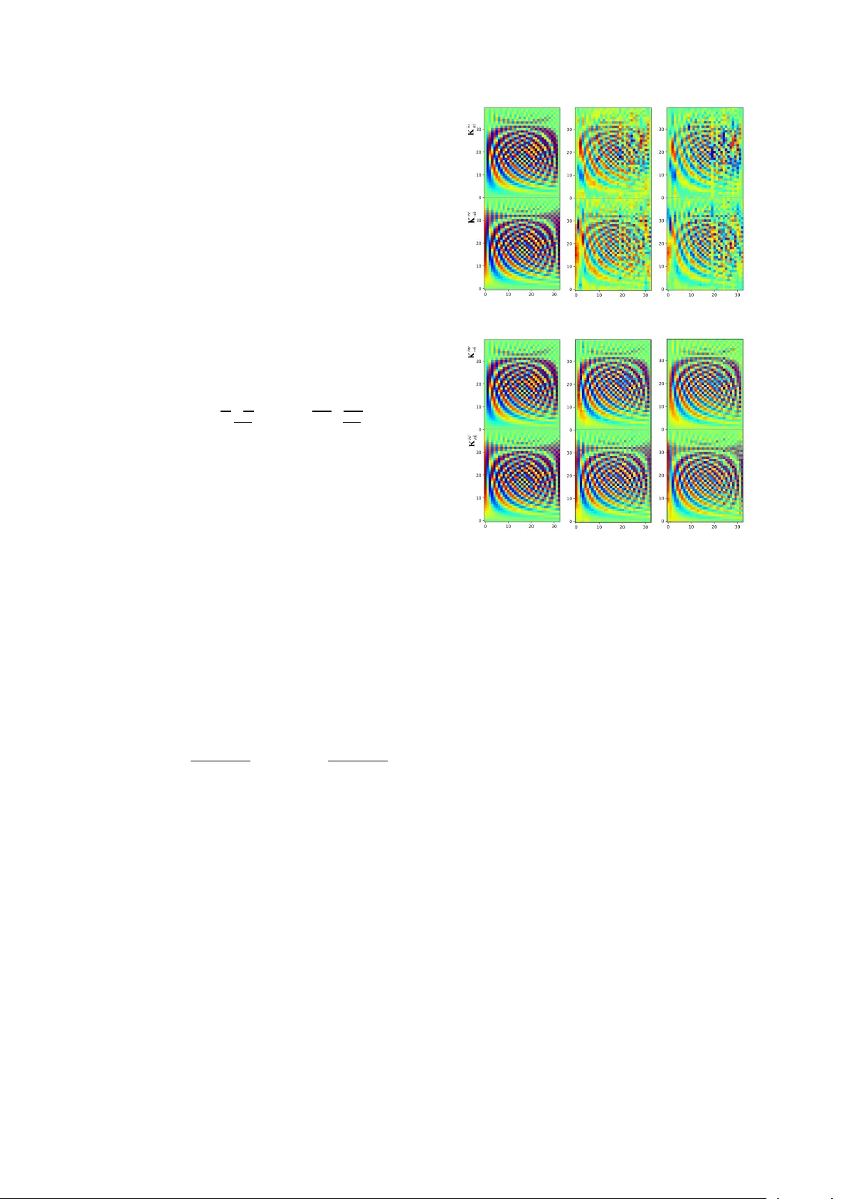
End-to-End Multi-Channel Speech Separation Rongzhi Gu ∗ 1 , 3 , Jian W u ∗ 2 , 3 , Shi-Xiong Zhang 4 , Lianwu Chen 3 , Y ong Xu 4 , Meng Y u 4 , Dan Su 3 , Y uexian Zou 1 , Dong Y u 4 1 Peking Uni versity Shenzhen Graduate School, Shenzhen, China 2 Northwestern Polytechnical Uni versity , Xi’an, China 3 T encent AI Lab, Shenzhen, China 4 T encent AI Lab, Belle vue W A, USA { zouyx, Moplast grz } @pku.edu.cn, jianwu@nwpu-aslp.org, { auszhang, lianwuchen, lucayongxu, raymondmyu, dansu, dyu } @tencent.com Abstract The end-to-end approach for single-channel speech separation has been studied recently and shown promising results. This paper extended the previous approach and proposed a ne w end- to-end model for multi-channel speech separation. The primary contributions of this work include 1) an integrated wav eform-in wa veform-out separation system in a single neural network ar - chitecture. 2) W e reformulate the traditional short time Fourier transform (STFT) and inter-channel phase difference (IPD) as a function of time-domain con v olution with a special kernel. 3) W e further relaxed those fixed kernels to be learnable, so that the entire architecture becomes purely data-driven and can be trained from end-to-end. W e demonstrate on the WSJ0 far- field speech separation task that, with the benefit of learnable spatial features, our proposed end-to-end multi-channel model significantly improved the performance of previous end-to-end single-channel method and traditional multi-channel methods. Index T erms : end-to-end, time-domain, multi-channel speech separation, spatial embedding 1. Introduction Lev eraging deep learning techniques, close-talk speech separa- tion has achiev ed a great progress in recent years. Several deep model based methods ha ve been proposed, such as deep cluster - ing [10, 12], deep attractor network [11], permutation inv ariant training (PIT) [8, 9], chimera++ network [13] and time-domain audio separation network (T asNet) [3, 4]. These approaches hav e opened the door towards cracking the cocktail party prob- lem. Howe ver , most of them operated on time-frequency (T - F) representation of raw wa veform signals after Short Time Fourier Transform (STFT). The computed spectrogram is in complex-v alued domain, which can be decomposed into magni- tude and phase part. Due to the dif ficulty on phase retriev al and human ears are insensitive to phase distortion to some extent, magnitude spectrogram is then a general choice for separation network to work with. The phase of speech mixture is used to combine with predicted magnitude to reconstruct waveforms. Currently , more researchers realized the negati ve influence of wa veform reconstruction using mixture phase and started to work on phase modeling and retrieving [18, 15, 16, 14]. For example, under an e xtreme condition when the mixture phase is opposite to the oracle phase, even though the magnitude is per- fectly predicted, the reconstructed wav eform is far away from Rongzhi Gu and Jian W u did this work when they were interns in T encent. They contributed equally to this w ork. the ground truth [17]. T o incorporate the phase into modeling, lots of efforts have been de voted to end-to-end methods which are conducted in time-domain [19, 3, 4]. T ypically , the con v olu- tional time-domain audio separation network (Con v-T asNet) [4] surpassed ideal T -F masking methods and achiev ed the state-of- the-art results on a widely used close-talk dataset WSJ0 mix. Although close-talk speech separation model achie ves great progress, the performance of far -field speech separation is still far from satisfactory due to the re verberation. A microphone ar- ray is commonly used to record multi-channel data. Correlation clues among multi-channel signals, such as inter-channel time difference, phase difference, level difference (ITD, IPD, ILD), can indicate the sound source position. These spatial features hav e been demonstrated to be beneficial, especially when com- bining with spectral features, for frequency-domain separation models [1, 2, 6, 5, 7]. Unfortunately , these spatial features (e.g., IPD) are hard to be incorporated in time-domain methods as they are typically extracted from frequency domain using dif- ferent analysis window type/length and hop size. In this work we propose a novel method to extract the spa- tial information from time domain using neural networks. This leads us to an inte grated wa veform-in w av eform-out system for multi-channel separation in a single neural network architec- ture that can be trained from end to end. This work can also be viewed as a multi-channel extension to the Con v-T asNet for time-domain far -field speech separation. The rest of paper is organized as follows. Section 2 re views previous end-to-end methods for single-channel speech separa- tion. Section 3 presents our end-to-end model for multi-channel speech separation. Experimental setup, implementation details and results are reported in Section 4 and 5. 2. Single-Channel End-to-End Separation There have been sev eral representative works for single-channel end-to-end speech separation. One of them is T asNet proposed by Luo et al. [3] which works in time domain for the speech sep- aration. The block diagram is illustrated in Figure 1. The net- work is designed as a encoder -decoder structure, where the C - mixed speech wav eform with S sampling points is decomposed on series of basis function to non-negativ e acti vations, which later can be inv erted back to the time-domain signal. Both the encoder and decoder are a Con v1D layer . The number of chan- nels N represents the number of basis functions. The kernel size L and stride L/ 2 are the window length and hop size, re- spectiv ely . The analysis windo w of T asNet is shortened from 32ms (512 sampling points) used in STFT -based methods to 5 Encoder Separator Decoder mixture representation W single-channel mixture waveform y speaker mask separated waveforms Figure 1: The bloc k diagram of T asNet. ms (80 sampling points). Bidirectional long short term memory (BLSTM) layers are adopted in the separation module which computes a mask from the encoded mixture representation for each source, similar to the T -F masking. Furthermore, instead of using a time-domain mean squared error (MSE) loss, the sep- aration metric scale-in variant signal-to-distortion (SI-SNR) is used to directly optimize the separation performance, which is defined as: SI-SNR := 10 log 10 k s target k 2 2 k e noise k 2 2 (1) where s target := ( h ˆ s , s i s ) / k s k 2 2 and e noise := ˆ s − s target are the estimated and clean source waveforms, respectiv ely . The zero- mean normalization is applied to s and ˆ s to guarantee the scale in v ariance and ˆ s , s ∈ R 1 × S . Recently , in [4], Luo et al. pointed out two major limits of LSTM networks. First, LSTM may have a long temporal dependency to handle the over growing number of frames with smaller kernel size, resulting accumulated error . The other is the computational complexity and large parameters of LSTM networks. T o alleviate the problems above, Luo proposed a improv ed version of T asNet, separator is replaced with a tem- poral fully-con v olutional network (TCN) [22]. The separation module consists of sequential layers that repeat R times of X stacked dilated Con v1D blocks, which supports a large recep- tiv e field in a noncausal setup. Meanwhile, in these dilated Con v1D blocks, the traditional conv olution is substituted with depthwise separable con v olution to further reduce the parame- ters. Another representativ e audio source separation work is W av e-U-Net [20], a multi-scale, end-to-end neural network in- troduced by Stoller et al. The model operates directly on the raw audio wav eform, which allo ws encoding the phase informa- tion. Multi-resolution features output from do wnsampling and upsampling blocks are computed and combined, which could incorporate long temporal context. In [14], end-to-end train- ing is also implemented by defining a time-domain MSE loss, where the T -F masking network is trained through an iterative phase reconstruction procedure. 3. Multi-channel End-to-End Separation Deep learning based multi-channel speech separation methods usually combine spectral features with inter-channel spatial fea- tures (e.g., IPD) [1, 2]. These IPD features hav e been proven effecti ve in many frequency domain frame works [5, 7]. The ra- tionale is that, the IPD computed by the STFT ratio of any two microphone channels will form clusters within each frequency , due to the source sparseness, for spatially separated directional sources with different time delays [26]. In section 3.1 we first try to incorporating the IPD features extracted from frequency domain into the T asNet. Then a cross-domain joint training is performed. In section 3.2 we reformulate the STFT and IPD as a function of time-domain con volution with special kernel. Then we relaxed those fixed kernels to be learnable. This leads us to an integrated wav eform-in wav eform-out system for multi- channel separation in a single neural network architecture that can be trained from end to end. 3.1. Cross-domain learning Firstly , we intend to integrate the well-established spatial fea- tures extracted in frequency domain to T asNet and jointly train the network. The block diagram is illustrated in Figure 2. Inspired by the dual-stream model applied in action recog- nition [ ? , 23, 24], the cross-domain feature fusion is feasible and effecti ve. In our particular case, the main branch for time- domain wa veform estimates speaker masks for the first chan- nel’ s mixture representation W . The frequency-domain fea- tures are extracted through performing STFT on each individ- ual channel of the mixture wa veform y ∈ R 1 × S to compute the complex spectrogram Y . Given a window function w with length T , the spectrum Y is calculated by: y [ n ] STFT − − → Y nk = T − 1 X m =0 y [ m ] w [ n − m ] e − i 2 πm T k (2) where n is the index of samples and k is the index of frequency bands. W e thereby compute IPD by the phase difference be- tween channels of complex spectrogram as: IPD ( u ) nk = ∠ Y u 1 nk − ∠ Y u 2 nk (3) where u 1 and u 2 represents two microphones’ indexes of the u -th microphone pair . Since the windo w length L in encoder is much shorter than windo w size T in STFT , upsampling is applied on the frequency domain features to match the dimen- sion of encoded mixture W . Since the mixture representa- Enco der Sepa rator Deco der 1 st chan ne l mixtu re wave fo rm y 1 spea ker ma sk sepa ra ted wav efo rms mixtu re rep resent ati on W con cat spati al em be dd ing E ( W , E ) STFT mult i - ch an ne l co mple x sp ec trogr am Y IPD IPD ca lc ul ati on (Eq. 3) ups amp le E Con v1 D mult i - ch an ne l co mple x rep res ent a tion IPD ca lc ul ati on (Eq. 6) E Cros s - doma in le ar nin g E nd - to - en d le ar ning Figure 2: The block diagram of our proposed multi-channel speech separation networks. The dashed boxes denotes the method described in Section 3.1 and Section 3.2, r espectively . The blocks marked in gr ey indicate the y are not in volved in network training. tion subspace and frequency domain do not share the same na- ture, frequency-domain features are encoded by an individual con v1 × 1 layer rather than directly concatenate with W . Also, apart from the early fusion method illustrated in Figure 2, which concatenates spatial embedding E with mixture representation before all 4 × 8 1D Con vBlocks in separator, we also in vestigate another tw o fusion methods, named middle fusion (after two in- dividual branches of 2 × 8 1D ConvBlocks) and late fusion (after two indi vidual branches of all 4 × 8 1D Con vBlocks). 3.2. End-to-End learning In the approach above, IPD features are computed using STFT with one pre-designed analysis window’ s type ( w ) and length ( T ) for all the frequency bands ( k ). At meanwhile, the time- domain encoder (see Fig. 2) automatically learns a serial of ker- nels in a data-driven fashion with dif ferent a kernel size and a stride size. This may cause a potential mismatch to the model. Motiv ated by this, the STFT in Eq. 2 can be reformulated as y [ n ] STFT − − → Y nk = phase factor z }| { e − i 2 πn T k ( y [ n ] ~ STFT kernel z }| { w [ n ] e i 2 πn T k ) (4) where n is the index of samples, k is the index of frequency bands and ~ is the con volution. This implies that we can com- pute the STFT using time-domain con volution with a special kernel. When compute the IPD between two microphones, one can substitute Eq. 4 into Eq. 3. Note the phase factor in Eq. 4 is constant between the corresponding frequency bands of two mi- crophones and thus can be cancelled out. This means the phase factor will neither affects the magnitude ( | · | = 1 ) nor IPD. The only thing matters to IPD features is the kernel in Eq. 4. Note the STFT kernel in Eq. 4 is a comple x number . It can be split in real and imaginary parts. K re nk = w [ n ] cos(2 π nk/T ) K im nk = w [ n ] sin(2 π nk/T ) (5) The shape of the kernel is determined by the w [ n ] . The size of the kernel is actually the window length T of w [ n ] . The stride of con volution equiv alents to the hop size in the STFT operation. Giv en the kernels, the u -th pair of IPD can be computed by: IPD ( u ) nk = arctan  y u 1 ~ K re nk y u 1 ~ K im nk  − arctan  y u 2 ~ K re nk y u 2 ~ K im nk  (6) Interestingly , although we derived the Eq. 4 and 5 from STFT , actually they can be generalize to any arbitrary kernels. This means we are not tied to a specific shape of kernel determined by w [ n ] , but any kernels that can be automatically learned from the data. Thus everything can be done in an integrated neural network (see Figure 2). Everything can be trained from end-to- end using the SI-SNR loss (Eq. 1). W e can also customize the number of kernels and use preferred kernel sizes other than T . The stride in con volution is also no w configurable other than just using the hop size of STFT . T o extract the IPD features directly from time-domain, all we need to do is to apply Eq. 6 with the kernel K re nk and K im nk we learned in each epoch. T o shed light on the properties of the kernel learning, Fig- ure 3 visualizes the learned kernels in different training stages. In the first column, kernel values are initialized with the STFT kernel in Eq. 5 but with a matched kernel size and stride with the encoder in Figure 2. In (a), along with the training, the kernels are unconstrained where K re nk and K im nk are separately learnable Epoch: 0 Epoch: 10 Epoch: 70 kernel index k kernel index k kernel index k value index n of value index n of (a) Epoch: 0 Epoch: 10 Epoch: 70 kernel index k kernel index k kernel index k (b) value index n of value index n of Figure 3: V isualization of learnable kernels in differ ent epochs. (a) unconstrained k ernels. (b) constrained kernel in the form of Eq. 5. The learned kernels are applied in Eq. 6 to compute IPD. parameters, therefore not conforming to the physical definition of the magnitude and phase of these k ernels. While in (b), w [ n ] in Eq. 5 is a trainable parameter so that the kernels try to learn a dynamic representation for the new “IPD” that is optimized for speech separation. 4. Experimental Setup 4.1. Dataset W e simulated a multi-channel reverberant version of two speaker mixed W all Street Journal (WSJ0 2-mix) corpus intro- duced in [10]. A 6-element uniform circular array is used as the signal receiver , the radius of which is 0.035m and these six microphones are placed with 60 degrees intervals. Each multi- channel two-speaker mixture is generated as follows. T wo speakers’ clean speech is mixed in the range from -2.5dB to 2.5dB. Then the classic image method is used to add multi- channel room impulse response (RIR) to the anechoic mixture and T60 ranges from 0.05 to 0.5 seconds. The room configura- tion (length-width-height) is randomly sampled from 3-3-2.5m to 8-10-6m. The microphone array and speakers are at least 0.3m away from the wall. W e do not add any constraints on the angle differences of speakers presence as [5, 7], so that our dataset contains samples of all ranges of angle differences, i.e., 0-180 degrees. All data is sampling at 16kHz. The mixing SNR, pairs, dataset partition are complete coincident with anechoic monaural WSJ0 2-mix. Note that all speakers in test set are unseen during training, thus our systems will be verified under T able 1: SI-SNR results (dB) of dif fer ent methods on spatialized r everber ant WSJ0 2-mix. Appr oach Input features Angle differences (°) A ve. < 15 15-45 45-90 > 90 T asNet (Con v) 1 st ch wa v 8.5 9.0 9.1 9.3 9.1 Freq-LSTM 1 st ch LPS + multi-channel IPD 3.0 6.7 7.9 8.2 6.9 Freq-BLSTM 1 st ch LPS + multi-channel cosIPD 6.5 9.0 9.4 9.0 8.7 Freq-TCN 1 st ch LPS + multi-channel cosIPD 5.6 8.6 8.7 8.3 8.0 cascaded networks 1 st ch LPS + multi-channel IPD 3.5 8.5 10.1 10.6 8.8 parallel encoder multi-channel wa v 5.7 10.3 11.9 12.9 10.8 cross-domain training 1 st ch wa v + LPS / early fusion 8.7 9.6 9.5 9.5 9.4 1 st ch wa v + LPS / middle fusion 9.2 9.7 9.6 10.0 9.7 1 st ch wa v + LPS / late fusion 8.7 9.4 9.3 9.5 9.3 1 st ch wa v + LPS + multi-channel cosIPD / middle fusion 8.3 11.4 11.7 11.3 11.0 end-to-end separation multi-channel wa v / fixed kernel / cosIPD 8.5 11.8 12.0 11.6 11.2 multi-channel wa v / fixed kernel / cosIPD + sinIPD 7.7 11.6 12.3 12.6 11.5 multi-channel wa v / trainable kernel (unconstrained) / cosIPD 7.9 11.3 12.0 11.3 11.0 multi-channel wa v / trainable kernel ( w [ n ] ) / cosIPD 8.2 11.6 12.0 11.4 11.1 multi-channel wa v / trainable kernel ( w [ n ] ) / cosIPD + sinIPD 7.9 11.6 12.5 12.9 11.6 IBM - 11.6 11.5 11.5 11.5 11.5 IRM - 11.0 11.0 11.0 11.0 11.0 IPSM - 13.7 13.6 13.6 13.6 13.6 speaker -independent scenario. 4.2. Network training and Feature extraction All hyper-parameters are the same with the best setup of Con v- T asNet, except L is set to 40 and encoder stride is 20. Batch nor- malization (BN) is adopted because it has the most stable per- formance. SI-SNR is utilized as training objecti ve. The training uses chunks with 4.0 seconds duration. The batch size is set to 32. The selected pairs for IPDs are (1, 4), (2, 5), (3, 6), (1, 2), (3, 4) and (5, 6) in all e xperiments. For cross-domain training, both LPS and IPDs are served as frequency domain features. These features are extracted with 32ms window length and 16ms hop size with 512 FFT points. For end-to-end separation, the num- ber of filters is set to 33 since we round the window length to the closest exponential of 2, i.e., 64. 4.3. Rival Systems Besides methods proposed in Section 3, we in vestigated several multi-channel speech separation approaches as baseline sys- tems. Also, we proposed a few alternativ e multi-channel sep- aration systems. Freq-LSTM/BLSTM . Sev eral works hav e proven the effec- tiv eness of inte gration of spatial and spectral features in LSTM- based frequency-domain separation networks [5, 7, 1]. For simiplicity , we call it Freq-LSTM. LPS and 6 pairs of IPD fea- tures are concatenated at input level and Freq-LSTM estimates a T -F mask for each speaker . The netw ork contains three LSTM layers with 300 cells, follo wed by a 512-node fully-connected layer with Rectified Linear Unit (ReLU) activ ation function. The output layer with sigmoid consists of 257 × 2 nodes as it outputs estimated masks for two speakers. Freq-TCN . W e replace the separation network used in Freq- LSTM with a TCN, which features long-range receptive field and deep extraction ability [21, 22], named Freq-TCN. Also, a 256-node BLSTM layer is appended after TCN to guarantee the temporal continuity of output sequence. The training craterion and output product is the same with Freq-LSTM. The repeat times and number of dilated blocks are change to 6 and 4. The detail of this system will be discussed in Appendix A. Cascaded Networks . One way of extending the time-domain methods (like T asNet) from single-channel to multi-channel, is to simply apply the traditional multi-channel frequency-domain method (like Freq-LSTM) first to incorporate the spatial infor- mation, then followed by single-channel T asNet. Refer to Ap- pendix C for the detailed description. Parallel encoder . In this method we replace the single encoder in Con v-T asNet with multiple parallel encoders to extract the mixture representation and spatial information simultaneously . The details are presented in Appendix B. 5. Result and Analysis SI-SNR improv ement (SI-SNRi) is used to measure the sep- arated speech quality as described in Section 2. Except the ov erall performance, we list results under different angle dif- ference ranges for comparisons. The results are presented in T able 1. W e repeat the single-channel Con v-T asNet and achiev e 15.2dB SI-SNRi compared to 14.6dB reported in [4] on close- talk WSJ0 2-mix dataset. The single-channel Con v-T asNet, Freq-LSTM, Freq-BLSTM and Freq-TCN are served as our baselines, respecti vely achie ves 9.1dB, 6.9dB, 8.7dB and 8.0dB on far-field WSJ0 2-mix dataset. F or reference, we also re- port the results achieved by ideal time-frequenc y masks, includ- ing ideal binary mask (IBM), ideal ratio mask (IRM) and ideal phase-sensitiv e mask (IPSM). These masks are calculated using STFT with a 512-point FFT size and 256-point hop size. Cascaded networks : Freq-LSTM alone achiev es 6.9dB, and Con v-T asNet refines the estimation and improves the perfor- mance to 8.8dB. The performance is slightly w orse than single- channel Con v-T asNet baseline, ho we ver , when the angle differ - ence is larger than 45°, it outperforms all baseline systems. Parallel encoder : The parallel encoder pushes the overall per- formance up to 10.8dB. It demonstrates the ef fectiv eness of data-driv en spatial coding and achieves the best performance among all systems for samples with angle dif ference lar ger than 90°. Ho wev er , the single-channel mixture representation seems not well preserved since the performance degrades on samples with small angle difference. Cross-domain training : Comparing to Con v-T asNet baseline, joint training with LPS feature slightly improves the perfor- mance for all angle differences. Besides, middle fusion outper- forms the other two fusion methods and achieves 9.7dB ov erall performance. W ith LPS and cosIPD features, both the spectral and spatial information is incorporated by cross-domain train- ing and the result is largely increased to 11.0dB. End-to-End separation : The con volution kernels enable IPD calculation inside the network, thus makes it an end-to-end ap- proach. With only cosIPD, fixing the kernels as initialized val- ues, i.e., DCT coef ficients, achiev e 11.2 dB SI-SNRi. Also, the performance of learnable kernels is slightly worse than the fixed ones. Howe ver , with the complementary information from sinIPD, the trainable kernel achie ves the best result among all systems, i.e., 11.6 dB, surpassing the performance of ideal bi- nary mask and ideal ratio mask. 6. Conclusions In this paper , we propose a new end-to-end approach for multi- channel speech separation. First, an integrated neural architec- ture is proposed to achie ve a wa veform-in wav eform-out speech separation. Second, W e reformulate the traditional STFT and IPD as a function of time-domain conv olution with a fixed spe- cial kernel. Third, we relaxed the fixed kernels to be learnable, so that the entire architecture becomes purely data-driven and can be trained from end-to-end. Experimental results on far - field WSJ0 2-mix validate the effecti veness of our proposed end-to-end systems as well as other multi-channel extensions. 7. References [1] Z. Chen, X. Xiao, T . Y oshioka, H. Erdogan, J. Li, and Y . Gong, “Multi-channel overlapped speech recognition with lo- cation guided speech extraction network, ” in 2018 IEEE Spoken Language T echnology W orkshop (SLT) . IEEE, 2018, pp. 558– 565. [2] T . Y oshioka, H. Erdogan, Z. Chen, and F . Alleva, “Multi- microphone neural speech separation for far-field multi-talker speech recognition, ” in 2018 IEEE International Conference on Acoustics, Speech and Signal Processing (ICASSP) . IEEE, 2018, pp. 5739–5743. [3] Y . Luo and N. Mesgarani, “T asnet: time-domain audio separation network for real-time, single-channel speech separation, ” in 2018 IEEE International Conference on Acoustics, Speech and Signal Pr ocessing (ICASSP) . IEEE, 2018, pp. 696–700. [4] Y . Luo and N. Mesgaran1, “T asnet: Surpassing ideal time- frequency masking for speech separation, ” arXiv pr eprint arXiv:1809.07454 , 2018. [5] Z.-Q. W ang, J. Le Roux, and J. R. Hershey , “Multi-channel deep clustering: Discriminative spectral and spatial embeddings for speaker-independent speech separation, ” in 2018 IEEE Interna- tional Confer ence on Acoustics, Speech and Signal Pr ocessing (ICASSP) . IEEE, 2018, pp. 1–5. [6] L. Drude and R. Haeb-Umbach, “Tight integration of spatial and spectral features for bss with deep clustering embeddings. ” in In- terspeech , 2017, pp. 2650–2654. [7] Z. W ang and D. W ang, “Integrating spectral and spatial features for multi-channel speaker separation, ” in Pr oc. Interspeech , vol. 2018, 2018, pp. 2718–2722. [8] D. Y u, M. K olbæk, Z.-H. T an, and J. Jensen, “Permutation inv ari- ant training of deep models for speaker-independent multi-talker speech separation, ” in 2017 IEEE International Confer ence on Acoustics, Speech and Signal Processing (ICASSP) . IEEE, 2017, pp. 241–245. [9] M. K olbæk, D. Y u, Z.-H. T an, J. Jensen, M. K olbaek, D. Y u, Z.-H. T an, and J. Jensen, “Multitalker speech separation with utterance- lev el permutation inv ariant training of deep recurrent neural net- works, ” IEEE/A CM T ransactions on Audio, Speech and Languag e Pr ocessing (T ASLP) , vol. 25, no. 10, pp. 1901–1913, 2017. [10] J. R. Hershey , Z. Chen, J. Le Roux, and S. W atanabe, “Deep clustering: Discriminative embeddings for segmentation and sep- aration, ” in 2016 IEEE International Conference on Acoustics, Speech and Signal Processing (ICASSP) . IEEE, 2016, pp. 31–35. [11] Y . Luo, Z. Chen, and N. Mesg arani, “Speak er-independent speech separation with deep attractor network, ” IEEE/A CM T ransactions on Audio, Speech, and Language Processing , vol. 26, no. 4, pp. 787–796, 2018. [12] Y . Isik, J. L. Roux, Z. Chen, S. W atanabe, and J. R. Hershey , “Single-channel multi-speaker separation using deep clustering, ” arXiv pr eprint arXiv:1607.02173 , 2016. [13] Z.-Q. W ang, J. Le Roux, and J. R. Hershey , “ Alternati ve objecti ve functions for deep clustering, ” in 2018 IEEE International Con- fer ence on Acoustics, Speech and Signal Processing (ICASSP) . IEEE, 2018, pp. 686–690. [14] Z.-Q. W ang, J. L. Roux, D. W ang, and J. R. Hershey , “End-to-end speech separation with unfolded iterativ e phase reconstruction, ” arXiv pr eprint arXiv:1804.10204 , 2018. [15] N. T akahashi, P . Agrawal, N. Goswami, and Y . Mitsufuji, “Phasenet: Discretized phase modeling with deep neural net- works for audio source separation, ” in Pr oc. Interspeech , 2018, pp. 2713–2717. [16] H.-S. Choi, J.-H. Kim, J. Huh, A. Kim, J.-W . Ha, and K. Lee, “Phase-aware speech enhancement with deep complex u-net, ” arXiv pr eprint arXiv:1903.03107 , 2019. [17] J. Le Roux, G. Wichern, S. W atanabe, A. Sarroff, and J. R. Her- shey , “Phasebook and friends: Leveraging discrete representa- tions for source separation, ” IEEE Journal of Selected T opics in Signal Pr ocessing , 2019. [18] P . Mowlaee, R. Saeidi, and R. Martin, “Phase estimation for signal reconstruction in single-channel source separation, ” in Thirteenth Annual Conference of the International Speech Communication Association , 2012. [19] S. V enkataramani, J. Casebeer, and P . Smaragdis, “ Adapti ve front- ends for end-to-end source separation, ” in Pr oc. NIPS , 2017. [20] D. Stoller , S. Ewert, and S. Dixon, “W ave-u-net: A multi-scale neural network for end-to-end audio source separation, ” arXiv pr eprint arXiv:1806.03185 , 2018. [21] C. Lea, M. D. Flynn, R. V idal, A. Reiter , and G. D. Hager , “T em- poral con volutional networks for action segmentation and detec- tion, ” in pr oceedings of the IEEE Confer ence on Computer V ision and P attern Recognition , 2017, pp. 156–165. [22] C. Lea, R. V idal, A. Reiter, and G. D. Hager, “T emporal conv o- lutional networks: A unified approach to action segmentation, ” in Eur opean Conference on Computer V ision . Springer, 2016, pp. 47–54. [23] K. Simonyan and A. Zisserman, “T wo-stream conv olutional net- works for action recognition in videos, ” in Advances in neural information pr ocessing systems , 2014, pp. 568–576. [24] C. Feichtenhofer , A. Pinz, and A. Zisserman, “Conv olutional two-stream network fusion for video action recognition, ” in Pro- ceedings of the IEEE conference on computer vision and pattern r ecognition , 2016, pp. 1933–1941. [25] S. V enkataramani, J. Casebeer, and P . Smaragdis, “End-to-end source separation with adaptive front-ends, ” in 2018 52nd Asilo- mar Conference on Signals, Systems, and Computers . IEEE, 2018, pp. 684–688. [26] S. Gannot, E. V incent, S. Markovich-Golan, and A. Ozerov , “A Consolidated Perspecti ve on Multi-Microphone Speech Enhance- ment and Source Separation, ” IEEE/ACM T ransactions on A udio, Speech, and Languag e Pr ocessing , vol. 25, pp. 692–730, 2017. A. A ppendix In this section, we describe three riv al systems in detail: Freq- TCN, cascaded networks and parallel encoder . A. Freq-TCN As sho wn in Figure 4, Freq-TCN shares the same processing architecture with Freq-LSTM except the separation network backbone structure. First, multi-channel mixture speech wave- form is transformed to complex STFT representation. Then, spectral and spatial features are extracted and served as the in- put of separation network, i.e., magnitude spectra and IPDs. For separation network, the LSTM layers are replaced with a tem- poral con volutional network (TCN), which features long-range receptiv e field and deep extraction ability [21, 22]. The TCN’ s structure is the same as that used in Con v-T asNet. Also, a 256- node BLSTM layer is appended after the TCN to guarantee the temporal continuity of output sequence. The separation mod- ule learns to estimate a time-frequency mask for each source in the mixture. The network training criterion is phase-sensitiv e spectrogram approximation (PSA): L P SA = C X c =1 k ˆ M ◦ | Y 1 | − | X c | ◦ cos ( ∠ Y 1 − ∠ X c ) k 2 F (7) where C indicates the number of speakers in the speech mix- ture, ˆ M is the phase-sensitive mask (PSM) estimated by the network, | X c | and ∠ X c is the magnitude and phase of the c -th source’ s complex spectrogram, respectiv ely . STFT Se pa rato r iSTFT | Y 1 | m ult i - chan ne l mi xture wavefo rm y spea ker ma sks sepa ra ted wav efo rms Y IPDs Figure 4: The bloc k diagram of F r eq-TCN. B. Cascaded Networks It’ s rather simple and facilitative to combine established spatial features such as IPDs with the spectral features in frequency domain. Several works have prov en the effecti veness of this integration in LSTM-based frequency-domain separation net- works. For conv enience, we call them Freq-LSTM methods. Thus, instead of bothering to explore exploitable spatial features in time-domain separation, we stack a Freq-LSTM network on the top of single-channel Con v-T asNet. The illustration of this method is shown in Figure 5. Specifically , under the supervision of ideal ratio mask (IRM), Freq-LSTM learns to estimate the magnitude mask for each source. Then, reconstructing with the mixture phase of the first channel mixture spectrogram, pre-separated wav eforms could be obtained by in verse STFT (iSTFT). Next, Con v-T asNet takes these tw o pre-separated wa veforms as input, and concate- nates their representation along feature dimension after the T as- Net’ s encoder . The separation module is targeted at generating a mask for each source’ s representation. In this approach, the multi-channel Freq-LSTM is served as a separation front-end, which takes both spatial and spectral feature into consideration and giv es a reasonable yet somewhat coarse estimation. The backend Con v-T asNet can refine the inaccurate phase and im- prov e the separation performance of these pre-estimated results, in view of its powerful separation capability in time-domain. Unfortunately , the inv erse STFT (iSTFT) operation hinders the joint training of Freq-LSTM and Con v-T asNet, thus accumu- lates estimation errors from each network. Also, the large mis- match between training and ev aluation dataset also impedes the av ailability of this method. Freq-LSTM T asNet pre-separated waveforms multi-channel mixture speech features estimated T -F masks separated waveforms iSTFT Y 1 Figure 5: The block diagram of cascaded networks, wher e the Y 1 denotes the first channel’ s complex spectr ogram of multi- channel mixtur e speech. C. Parallel Encoder T o automatically dig out cross-correlations between channels of multi-channel speech, we adopt a parallel encoder instead of a single encoder, as illustrated in Figure 6. The parallel en- coder carries out wav eform encoding and cross-channel cues extraction as well. This parallel encoder contains N con volu- tion kernels for each channel of the input multi-channel speech mixture y and sums the conv olution output across channels to form mixture feature maps. The follo wing steps are the same with single-channel Con v-T asNet. Encoder Separator Decoder mixture representation W multi-channel mixture waveform y speaker mask separated waveforms Encoder Encoder ... + Figure 6: The bloc k diagram of par allel encoder .