A Low-Cost Robust Distributed Linearly Constrained Beamformer for Wireless Acoustic Sensor Networks with Arbitrary Topology

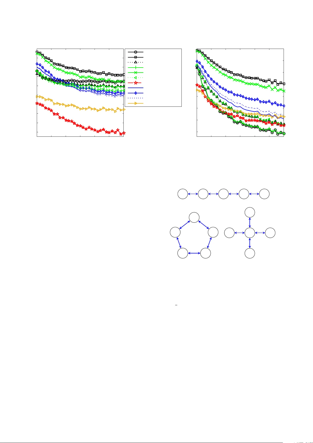
1 A Lo w-Cost Rob ust Distrib uted Linearly Constrained Beamformer for W ireless Acoustic Sensor Networks with Arbitrary T opology Andreas I. K outrouvelis, Thomas W . Sherson, Richard Heusdens and Richard C. Hendriks Abstract —W e propose a new robust distributed linearly con- strained beamformer which utilizes a set of linear equality constraints to reduce the cr oss power spectral density matrix to a block-diagonal form. The proposed beamformer has a con venient objective function for use in arbitrary distributed network topologies while having identical perf ormance to a centralized implementation. Moreover , the new optimization problem is rob ust to relative acoustic transfer function (RA TF) estimation errors and to target activity detection (T AD) errors. T wo variants of the proposed beamf ormer are presented and e valuated in the context of multi-micr ophone speech enhancement in a wireless acoustic sensor network, and are compared with other state-of- the-art distributed beamformers in terms of communication costs and robustness to RA TF estimation errors and T AD errors. Index T erms —Distributed beamforming, LCMV , MVDR, ro- bust beamforming, speech enhancement, W ASN. I . I N T RO D U C T I O N B EAMFORMING (see e.g., [1]–[3] for an ov erview) plays an important role in multi-microphone speech enhance- ment [4]–[7]. The aim of a beamformer is the joint suppression of interfering noise and the preserv ation of an unknown target signal. The increasing usage of wireless portable devices equipped with microphones and limited power supplies, makes the notion of distributed beamforming in wireless acoustic sensor networks (W ASNs) attracti ve compared to traditional centralized implementations [8]. The last decade, there are sev eral proposed low-complexity distrib uted beamformers [9]– [18] that mainly focus on achieving a good trade-off between noise reduction and communication cost. Both centralized and distributed beamformers typically re- quire an estimate of the cross-power spectral density matrix (CPSDM) of the noise/noisy measurements, and estimate(s) of the relativ e acoustic transfer function (RA TF) vector(s) of the acoustic source(s) present in the acoustic scene. Estimation errors in these quantities result in performance degradation of beamformers. Much attention has therefore been giv en to the development of centralized robust beamformers which minimize the effects of RA TF estimation errors (see e.g., [2], [3] for an overvie w). Dev eloping robust distributed beam- formers is more challenging than de veloping rob ust central- ized beamformers, as distributed beamformers cannot afford high-complexity robust solutions. Therefore, it is desired to ﬁnd very low-comple xity robust distributed beamformers that achiev e good performance trade-offs as described previously . A low-comple xity and easily manipulated family of beam- formers are those that are calculated through linearly con- strained quadratic problems such as: the minimum power dis- tortionless responce (MPDR) beamformer [19] and its multiple constrained generalization, the linearly constrained minimum power (LCMP) beamformer [20]. Both beamformers minimize the total po wer of the noisy measurements while preserving the target. Therefore, their performance highly depends on the estimation accuracy of the RA TF vector of the target source [2], [3], [21]. RA TF estimation errors might result in remov al of the actual tar get source and preservation in the direction of the wrongly estimated RA TF vector . T wo straightforward, low-complexity , robust alternatives to MPDR and LCMP are the minimum variance distortionless re- sponse (MVDR) beamformer [21] and the linearly constrained minimum variance (LCMV) beamformer [2], respectively . Both methods minimize the output noise power instead of the total noisy power , and thus require an estimate of the noise- only CPSDM. The noise CPSDM is typically estimated using a target acti vity detector (T AD) to identify tar get-free time- segments of audio. When the tar get is speech, this typically takes the form of a voice acti vity detector (see e.g., [6] for an overvie w). In [22], an alternativ e method was proposed to track the noise CPSDM also in time regions where the target is present. This method, howe ver , highly depends on the estimation accuracy of the RA TF vector of the target and its robustness to RA TF estimation errors has not been tested. Another family of low-comple xity , robust alternatives to MPDR and LCMP are their diagonal loaded versions (see e.g., [23]–[25]). In both versions, the diagonal loading pa- rameter , which is added to the main diagonal of the CPSDM, trades-off robustness against noise suppression. Speciﬁcally , by increasing the value of the diagonal loading parameter, a higher robustness to RA TF estimation errors and a lower noise suppression is achie ved. W ith diagonal loading, the use of a T AD is unnecessary . T o the authors’ knowledge, there are no low-comple xity distrib uted approaches for choosing the optimal diagonal loading parameter . Additionally , a constant diagonal loading parameter will not be optimal for all acous- tical scenarios and all frequency bins. From the above it becomes clear that in addition to ro- bustness and lo w-cost distributed calculations, LCMV and LCMP beamformers have the additional challenge of the RA TF vector estimation of the target source and possibly the interferers. There are several centralized methods for RA TF vector estimation (see e.g., [7] for an overvie w), howev er, there are yet no low-comple xity distributed alternativ es for arbitrary network topologies. In several applications, such as 2 teleconferencing, the sources do not change their locations signiﬁcantly ov er time and, therefore, one may estimate the RA TF vectors of the target and/or the interferers only during initialization using a centralized approach and then use these estimated RA TF vectors in the distributed beamformer . The slight positional errors that will most likely occur after this initial estimation require robust distributed beamformers. Note that in this paper , we mainly focus on this type of applications, i.e., the sources that do not signiﬁcantly change their locations with respect to an initial reference location. Notably , existing distributed beamformers can be classiﬁed based on how they address the issue of forming CPSDMs in W ASNs. In the ﬁrst class, the CPSDMs are approximated to form distributed implementations [9]–[12] leading to approxi- mately optimal performance. In the second class, the proposed beamformers obtain statistical optimality but do so at the expense of restricting the topology of the underlying W ASN [13]–[15]. Statistically optimal beamformers which operate in unrestricted network topologies are much less common. An early example of such a beamformer is provided in [16], based on a maximum likelihood estimated LCMP beamformer . Un- fortunately , this approach suffers from scaling communication costs as the number of samples used to construct the estimated CPSDM increases. In a similar vein, in [26], a distributed beamformer based on the pseudo-coherence principle was proposed. Similar to [16], the method in [26] can operate in cyclic networks. Furthermore, the authors demonstrated ho w the algorithm could perform near optimally with only a ﬁnite number of iterations, resulting in lo w transmission complexity . More recently , in [18] a topology independent distributed beamformer (i.e. able to operate in cyclic networks) was proposed. Similar in its design to [14], this method requires very limited communication between nodes while guarantee- ing con ver gence to the optimal beamformer . Howe ver , it was also demonstrated that the rate of this conv ergence was slow , requiring a large number of iterations to achiev e this point. In practice, with even slowly varying sound ﬁelds such a rate of con vergence may be detrimental to ov erall performance. In this paper, we propose a ne w robust distributed linearly constrained beamformer, addressing the aforementioned chal- lenges. The optimization problem of the proposed method nulls each interferer using a linear equality constraint, reducing the full-element noise or noisy CPSDM to a block-diagonal form. In contrast to MVDR, MPDR, LCMV and LCMP beamformers, the proposed objectiv e function does not tak e into account correlation between different nodes in the W ASN. Additionally , such an objecti ve function is more con venient for distributed beamforming in W ASNs of arbitrary topologies and signiﬁcantly reduces the communication costs therein. W e show under realistic conditions, i.e., when the algo- rithms use non-ideally estimated RA TF vectors and a non-ideal T AD, that the proposed method achieves a better predicted intelligibility than the MVDR and LCMV . The proposed method is less sensiti ve to RA TF estimation errors, when T AD errors are not negligible, because of the block-diagonal form of the CPSDM. The remainder of the paper is or ganized as follows. Sec- tion II presents the signal model. Section III revie ws sev eral methods of estimating the RA TF vectors of the sources and the noisy/noise CPSDMs. Section IV revie ws the centralized and distributed linearly constrained beamformers. Section V presents the centralized and distrib uted versions of the pro- posed method. Section VI shows the experimental results. Finally , concluding remarks are drawn in Section VII. I I . S I G NA L M O D E L Consider an arbitrary undirected W ASN of N nodes. W ith- out loss of generality , we assume that the underlying net- work (which is potentially c yclic) is connected. Denote by V = { 1 , · · · , N } the set of node indices and by E the set of edges of the netw ork whereby ( i, j ) ∈ E ⇐ ⇒ i, j ∈ V , i 6 = j can communicate with one another . Each node κ is equipped with M κ microphones, where P κ ∈ V M κ = M , thus forming an M -element microphone array . One of the M microphones is selected as the reference microphone for the beamforming purpose. The distributed beamformers presented in this paper are formulated in the short-time Fourier transform (STFT) domain on a frame-by-frame basis. The noisy DFT coefﬁcient of the j -th ( j = 1 , · · · , M ) microphone of the k -th frequency bin of the β -th frame is given by y j ( k , β ) = a j ( k , β ) s ( k , β ) | {z } x j ( k,β ) + r X i =1 b ij ( k , β ) v i ( k , β ) | {z } n ij ( k,β ) + u j ( k , β ) (1) with s ( k , β ) and v i ( k , β ) the target source and the i -th interferer at the reference microphone, a j ( k , β ) and b ij ( k , β ) the RA TF vectors elements of each with respect to the j -th microphone, and x j ( k , β ) , n ij ( k , β ) and u j ( k , β ) the target source, the i -th interferer and ambient noise at the j -th microphone. Note that the reference microphone element of the RA TF vectors is always equal to 1 . Moreov er, in the case of rev erberant en vironments, the RA TF vectors may also include a component due to early re verberation [27], [28]. Late rev erberation and microphone self-noise are typically included in the ambient noise component. Note that ev en the late rev erberation of the tar get has to be assigned to the ambient noise component because it reduces intelligibility [29], [30]. Thus, it should be reduced via the use of the beamformer . Howe ver , the early reﬂections (typically the ﬁrst 50 ms [30]) are desired to be maintained because they typically contribute to intelligibility [29], [30]. Therefore, the ambient noise com- ponent is given by u j ( k , β ) = l s j ( k , β ) + r X i =1 l v i j ( k , β ) + c j ( k , β ) , where l s j ( k , β ) is the late rev erberation component due to the target, l v i j ( k , β ) is the late reverberation component due to the i -th interferer , and c j ( k , β ) is the microphone self-noise. In the sequel, we neglect the frame and frequency indices for the sake of bre vity . Stacking all variables into vectors, Eq. (1) can be rewritten as y = x + r X i =1 n i + u | {z } n ∈ C M × 1 . 3 The CPSDM of y is given by P y = E [ yy H ] , where E [ · ] de- notes statistical expectation. Assuming all sources are mutually uncorrelated, we have P y = P x + r X i =1 P n i + P u | {z } P n ∈ C M × M , (2) where P x = E [ xx H ] = p s aa H and P n i = E [ n i n H i ] = p v i b i b H i are the CPSDMs of the target source and the i -th interferer at the microphones, respectively . Note that p s and p v i are the po wer spectral densities of the tar get and the i - th interferer , respecti vely . Finally , the CPSDM of the ambient noise component, P u , is given by P u = E [ uu H ] = P l s + r X i =1 P l u i | {z } P l + P c ∈ C M × M , where P l denotes the CPSDM of the late reverberation, and P c the CPSDM of the microphone self-noise. I I I . E S T I M A T I O N O F S I G NA L M O D E L P AR A M E T E R S The CPSDMs and the RA TF vectors of the sources are unknown and hav e to be estimated in order to be available to the beamformers discussed in the sequel. In Sections III-A and III-B, we revie w some existing methods for RA TF vector and CPSDM estimation, respectively . A. Estimation of RA TF V ectors In practical applications, the true RA TF vectors are re- verberant due to room acoustics [28], [31], [32]. Several centralized methods hav e been proposed to estimate these RA TF vectors (see e.g., [7] for an overvie w). In [28], the RA TF vector of the target source is estimated by e xploiting the assumption that the noise ﬁeld is stationary . Ho wever , when the interferers are non-stationary , this can result in signiﬁcant degradation in performance [31]. In [32] the subspaces of the target and interferers are estimated using a generalized eigen value decomposition (GEVD) combined with a T AD. While distributed methods have been proposed in the literature for performing GEVD-based subspace estimation in restricted network topologies (i.e., fully connected) [33], to our best knowledge, there are currently no distributed versions of the GEVD that operate in general cyclic networks. In this work, we assume that estimates of the RA TF v ectors, ˆ a and ˆ b i , for i = 1 , · · · , r , are av ailable at the initialization phase. In situations where the sources do not change their lo- cations signiﬁcantly with respect to an initial position, such as teleconferencing, the RA TF vectors can be estimated (e.g., in a centralized way) during such an initialization. This will result in RA TF estimation errors if the sources make some slight mov ements and, therefore, robust beamformers are required. B. Estimation of CPSDMs The LCMP and the MPDR beamformers depend on an estimate of the noisy CPSDM, ˆ P y . T ypically , this estimate is computed using the sample average, which is giv en by ˆ P y = 1 | L y | X l y ∈ L y y ( l y ) y H ( l y ) , where L y is the set of frames of the entire time horizon and | · | denotes the cardinality of a set. The LCMV and the MVDR beamformers depend on an estimate of the noise CPSDM, ˆ P n . The noise CPSDM is estimated using the set of noise-only frames denoted by L n , i.e., ˆ P n = 1 | L n | X l n ∈ L n y ( l n ) y H ( l n ) , where | L n | < | L y | . In order to obtain ˆ P n , a T AD is required to detect target presence/absence for each frame. The abov e two av erages are updated in an online fashion, i.e., the av erage is updated for ev ery frame using the average of the previous frame. This procedure becomes computationally demanding in a distributed context for two reasons. Firstly , the entire observation vector must be av ailable at each time frame resulting in the need for data ﬂooding. Secondly , that the storage of the entire CPSDM scales with the network size. Estimation of the ambient noise CPSDM P u is a difﬁcult task due to the late reverberation CPSDM P l . Using a T AD it is nearly impossible to estimate P l alone. For suf ﬁciently large rooms, the late reverberation is typically modelled as an ideal spherical isotropic noise ﬁeld [7], [34].That is, ˆ P l = ˆ p iso P iso , (3) where for the k -th frequency bin, the ( i, j ) -th element of P iso is gi ven by P iso ,i,j = sinc  2 π kf s d i,j Φ c  , (4) where d i,j is the distance between microphones i and j , f s is the sampling frequency , Φ is the number of frequency bins, and c is the speed of sound. The scaling ˆ p iso can be estimated using sev eral centralized methods (see e.g., [34]). T o the best of our knowledge, there are no distributed methods for obtaining ˆ p iso . Fig. 1 shows the v alues of the correlation function of Eq. (4) for various frequencies and distances d i,j . The correlation can be roughly di vided into two interesting frequenc y regions: one highly correlated on the left and one much less correlated on the right. The boundary between these regions occurs at the ﬁrst zero-crossing gi ven by f c = c/ (2 d i,j ) . It is clear that, the larger d i,j becomes, the smaller f c is. The CPSDM of the microphone self-noise, P c = c I (where c is the power at each microphone), can be estimated in silent frames only (i.e., neither target nor interferers are active). I V . L I N E A R LY C O N S T R A I N E D B E A M F O R M I N G Most linearly constrained beamformers are obtained from the follo wing general optimization problem [1], [2], [20] ˆ w = ar g min w w H Pw s.t. w H Λ = f H , (5) 4 0 4 8 frequency (kHz) 0 0.5 1 P iso,i,j d i,j = 50 cm d i,j = 4 cm Fig. 1: The spherically isotropic noise ﬁeld correlation between two microphones i, j of distances d i,j = 4 , 50 cm and f s = 16 kHz. The star marker denotes the ﬁrst zero-crossing f c . where Λ ∈ C M × d , f ∈ C d × 1 , and P ∈ C M × M is typically the CPSDM of the noise or noisy measurements. The d constraints used in the optimization problem of Eq. (5) include at least the distortionless constraint for the target source, i.e., w H a = 1 , and, commonly , the nulling of the interferers, w H b i = 0 [1], [32], [35]. If we assume that r < M − 1 , the linearly constrained beamformer can null all interferers and still hav e control on the minimization of the objecti ve function. In this case, Λ and f are given by Λ =  a b 1 · · · b r  , and f =  1 0 · · · 0  H . (6) It should be noted that by increasing the number of nulling constraints, the ambient output noise power may be boosted. The boost depends on the locations of the interferers [2] and the number of av ailable degrees of freedom ( M − r − 1 ). Howe ver , in applications when r  M − 1 this impact is much less signiﬁcant. If r < M − 1 and P is inv ertible, the optimization problem in Eq. (5), using the constraints in Eq. (6), has a closed-form solution given by [2] ˆ w = P − 1 Λ  Λ H P − 1 Λ  − 1 f . When P = P y , the linearly constrained beamformer takes the form of the LCMP beamformer given by ˆ w = ar g min w w H P y w s.t. w H Λ = f H , (7) while if P = P n , the LCMV is obtained and is giv en by ˆ w = ar g min w w H P n w s.t. w H Λ = f H . In the sequel, when we use the acronyms LCMV and LCMP we mean the LCMV and LCMP versions with the constraints giv en in Eq. (6). Another interesting linearly constrained beamformer is the one that has only the ambient noise com- ponent in the objective function [36], i.e., ˆ w = ar g min w w H P u w s.t. w H Λ = f H . (8) In this paper , we will refer to the linearly constrained beam- former in Eq. (8) as the ambient LCMV (ALCMV). Using Eq. (2), the objecti ve function of the LCMP problem, as noted in Eq. (7), is given by w H P y w = p s w H aa H w + r X i =1 p v i w H b i b H i w + w H P u w . Due to the included constraints in the LCMP (see Eq. (6)), the contributions of the early components of the sources to the objective function of Eq. (7) are constant. Thus, if ˆ P y = P y , ˆ P n = P n , ˆ P u = P u , and ˆ Λ = Λ , the LCMP , LCMV and ALCMV beamformers are all equiv alent. In practice, this nev er happens as there are always RA TF estimation errors and CPSDM estimation errors, as explained previously . A. RATF estimation err ors There are two interesting cases. In the ﬁrst case, if ˆ P y = P y , ˆ P n = P n , and ˆ a = a , LCMP is equi valent to LCMV [2]. Howe ver , if ˆ a 6 = a , the LCMV beamformer (provided that ˆ P n is accurately estimated), is more rob ust than the LCMP [2]. This is because LCMP will try to remove the actual target related to the RA TF a as this is included in P y , while the preservation constraint is on the wrongly estimated ˆ a . Howe ver , if there are also T AD errors, ˆ P n may also contain portions of P x and, as a result, the LCMV may also ha ve sev ere performance degradation like the LCMP . In the second case, if ˆ P n = P n , ˆ P u = P u , and ˆ b i = b i , for i = 1 , · · · , r , LCMV is equi valent to ALCMV . Howe ver , if any of the ˆ b i ’ s contain estimation errors, there will be po wer leakage of the corresponding interferer(s), which is not controllable, neither by the objectiv e function nor by the constraints of the ALCMV problem in Eq. (8). Moreover , if there are interferers whose RA TF v ectors hav e not been placed in the constraints, the ALCMV will also be unable to reduce them in a controlled way . In contrast, if ˆ P n is estimated accurately , the LCMV will reduce these po wer leakages. In this case, the LCMV will most likely have a better noise reduction performance than its ALCMV counterpart. W e can conclude that the performance de gradation of lin- early constrained beamformers due to RA TF estimation errors is mainly inﬂuenced by the selection of the CPSDM, P , in the objecti ve function of Eq. (5). A lo w-cost rob ust linearly constrained beamformer should have good performance under both RA TF estimation errors and T AD errors. There are se veral approaches to achiev e this. The most popular is via diagonal loading of P . Howe ver , to the authors’ kno wledge there are no lo w-cost distributed approaches for optimally selecting the diagonal loading v alue. Another rob ust low-cost option is to use a ﬁxed superdirective linearly constrained beamformer, i.e., a linearly constrained beamformer with a (semi)ﬁxed P [5]. A ﬁxed linearly constrained beamformer does not use a T AD and guarantees that there will not be any portion of P x in P . T wo interesting ﬁxed linearly constrained beamformers are discussed in the next section. B. F ixed Super directive Linearly Constrained Beamformers The ﬁxed superdirectiv e beamformers [5] assume a cer- tain noise ﬁeld and use in the objectiv e function a certain coherence function like the one in Eq. (3). Since the early components of the interferers can be nulliﬁed using a linearly constrained beamformer, the noise ﬁeld that remains is the late rev erberation as explained pre viously in this section. Recall from Section III-B, that the estimation of P u is a difﬁcult task due to the CPSDM of the late rev erberation, P l . T ypically , in 5 the literature (see e.g., [5], [37], [38]) models of P l are used in beamformers instead. The most common choice is to use P iso . If one chooses P = P iso , the microphone self-noise will be boosted in lo w frequencies [5]. Thus, a diagonal-loaded version is typically used [5], [39], i.e., ˆ w = ar g min w w H ( p iso P iso + P c ) w s.t. w H Λ = f H , (9) where P c = c I (see Section III-B). Although, the microphone- self noise power , c , typically remains constant over time, p iso changes. T o the best of our knowledge, there are no distributed estimation methods of the scaling coefﬁcient p iso . W e call the beamformer in Eq. (9) as isotropic LCMV (ILCMV). Another popular ﬁxed linearly constrained beamformer uses in the objectiv e function the most simplistic option which is P = I , i.e., ˆ w = ar g min w w H w s.t. w H Λ = f H . (10) In this paper , we will refer to this as the linearly constrained delay and sum (LCDS) beamformer . It is identical to the ﬁxed beamformer of the generalized side-lobe canceller im- plementation of the LCMP beamformer (using the constraints in Eq. (6)) in [32]. Unlike ILCMV , the LCDS is easily distributable due to the separable nature of the objectiv e function. This can be achiev ed via similar methods to those demonstrated in Section V -C and need only be performed once. Follo wing this, the output can be computed via data aggregation or by solving a simple averaging problem, again lending itself to distributed implementations. Similar to ALCMV , the ILCMV and LCDS beamformers cannot control power leakages due to inaccurate estimates of the interferers’ RA TF vectors and cannot control interferers which are not included in the constraints. C. Other Related Linearly Constrained Beamformers If we skip the nulling constraints and only impose the target distortionless constraint, the LCMV (LCMP) reduces to the MVDR (MPDR) [1], [19]. Similar to LCMV and LCMP , MVDR and MPDR are equiv alent under the assumption that ˆ P y = P y and ˆ P n = P n and ˆ a = a [2]. Howe ver , when ˆ a 6 = a , the MVDR is more robust to RA TF estimation errors [2], [21]. A special case of the MPDR is the delay and sum (DS) beamformer [27] which replaces the noisy CPSDM with the identity matrix. The DS has worse performance compared to the MVDR (MPDR) in correlated noise ﬁelds but results in very robust performance to RA TF estimation errors [21] and T AD errors. D. Distributed Linearly Constrained Beamformers The de velopment of distributed beamformers has focused on adapting LCMV (LCMP) based approaches for use in W ASNs. Howe ver , this adaptation has not come without additional challenges [40]. Most notable is the limited communication between de vices which makes the formation of estimated CPS- DMs nearly impossible without the use of a fusion center [8]. T o address this, two main classes of distributed beamformers hav e appeared in the literature: approximately optimal v ariants and optimal approaches which operate in certain networks. One such sub-optimal variant is the distributed DS beam- former introduced in [9]. Based on randomised gossip [41], this low-cost method operates in general cyclic networks but fails to exploit spatial correlation to improve noise reduction. In contrast, distributed approximations of the MVDR beam- former [10], [11] assume that disjoint nodes are uncorrelated essentially masking the true CPSDMs. While lending them- selves to distributed implementations, such approaches fail to take into account the true correlations between observed sig- nals across the network, resulting in sub-optimal performance. By restricting the network topology , typically to be acyclic or fully connected, optimal distributed beamformers have been proposed. These algorithms [14], [15] exploit efﬁcient data ag- gregation to construct global beamformers from a composition of local ﬁlters and have been shown to be iterativ ely optimal. Howe ver , the additional communication overhead required to maintain a constant network topology across frames can be prohibitiv ely expensiv e due to unpredictable network dynam- ics. Furthermore, such maintenance may be impossible in the case of node failure. It is worth mentioning that it is not the use of an acyclic network in [14], [15] itself which is limiting, b ut rather the need for this network to be in variant ov er time. In [18], this point was exploited to form a fully distributed beamformer for use in general cyclic topologies. Like [14] and [15], [18] constructs a global beamformer as a composition of local beamformers at each node. Importantly , the method by which these local beamformers are combined does not depend on the underlying network topology . This allows the network to vary between frames, ov ercoming the need for maintaining a ﬁxed topology in all time instances. The method in [18] was shown to be iterativ ely optimal with its main drawback being a decrease in con ver gence rate compared to [14], requiring a larger number of frames to obtain near optimal performance. In contrast, in [16], an optimal distributed beamformer was proposed for use in cyclic networks by exploiting the structure of estimated CPSDMs to cast LCMP beamforming as distributed consensus. Ho wev er, for CPSDM estimates based on a large number of frames, the proposed algorithm’ s communication cost scaled poorly . In contrast to [13]–[15] and [18], a beneﬁt of [16] was that the proposed implementation was frame-optimal, i.e. that it obtained the performance of an equiv alent centralized implementation in each frame. The beamformer proposed in [26] e xploited a similar method of distributed implementation, but e xploited the pseudo coher- ence principle of human speech to ov ercome the scaling communication costs found in [16]. The approaches of both [16] and [26] made use of inter - nal optimization schemes which require a large number of iterations per frame to obtain optimal performance. Howe ver , in [26] it was shown that near optimal performance could be obtained using only a ﬁnite number of iterations of this internal solver . Such a result raises the question whether a similar approach could be employed as a general w ay of reducing the transmission costs associated with cyclic beamforming methods. For the beamformers proposed in this work, this 6 point is touched upon in Section V -G. In contrast to the methods above, the beamformers pro- posed in Section V are fully distributable without imposing restrictions on the underlying network topology or scaling communication costs while also being optimally computable in each frame. In this way , the proposed methods combine the strengths of e xisting distributed beamformers while also av oiding their various limitations. V . P R O P O S E D M E T H O D In the pre vious section, we ha ve highlighted the suscep- tibility of sev eral existing beamformers to RA TF estimation errors and T AD errors and the challenge of deploying these algorithms in distributed contexts. Here, we propose two dif- ferent linearly constrained beamformers which are efﬁciently distributable for arbitrary network topologies, robust to RA TF estimation errors and T AD errors, while at the same time are able to control the power leakage of the interferers. T ypically , the microphones within a node are nearby , while the microphones from different nodes are further away . There- fore, the late rev erberation will be highly correlated in the ﬁrst case, while in the latter less correlated (see Fig. 1). Therefore, providing that the nodes are sufﬁciently far away from each other , one may approximate the full element matrix P u with the block-diagonal matrix ¯ P u where ev ery block corresponds to the CPSDM of the late reverberation of one node only and the microphone-self noise. Therefore, we propose the block- diagonal ALCMV (BDALCMV) which is giv en by ˆ w = ar g min w w H ¯ P u w s.t. w H Λ = f H . (11) Note that if e very node has only one microphone, ¯ P u becomes diagonal. This block-diagonalization lends itself to distributed implementations, reﬂecting a similar objecti ve structure to that of the DS and LCDS beamformer . While the proposed BD ALCMV beamformer has a number of beneﬁts from the perspective of distributed signal pro- cessing, like ALCMV , the challenge becomes the estimation of ¯ P u , and handling the possible power leakages of the interferers as in the case of DS, LCDS, ALCMV . Therefore, in Sections V -A, and V -B we introduce two variations of the BD ALCMV beamformer which do not require the estimation of ¯ P u and are rob ust to power leakages of the interferers. Moreov er , in Sections V -C—V -G, we introduce distributed implementations of the proposed beamformers. A. BDLCMP Beamformer The ﬁrst proposed practical v ariant of BD ALCMV is the BDLCMP which uses in the objectiv e function the block- diagonal noisy CPSDM, ¯ P y . That is, ˆ w = ar g min w w H ¯ P y w s.t. w H Λ = f H . (12) This results in a local estimation problem, which can be carried out independently at each node without the need of a T AD. This method handles the possible power leakages due to inaccurate estimates of the interferers’ RA TF vectors and can suppress the interferers that are not included in the constraints. In case of RA TF estimation errors of the target source, the BDLCMP will hav e similar problems to the LCMP because in the block-diagonal matrices, there will be portions of the corresponding target block-diagonal CPSDMs. Howe ver , the performance degradation will not be that great as with the LCMP . This can be easily explained by considering the extreme scenario of a fully correlated noise ﬁeld in which we assume that M > r + 1 , ˆ P y = P y , P u ≈ 0 , ˆ b i = b i , i = 1 , · · · , r and ˆ a 6 = a . In this case, the optimization problem of LCMP in Eq. (7) will be approximately equiv alent 1 to the following optimization problem: ˆ w = ar g min w w H ˆ P y w s.t. w H ˜ Λ = ˜ f H , where ˜ Λ =  ˆ a a ˆ b 1 · · · ˆ b r  , and ˜ f H =  1 0 0 · · · 0  . That is, the LCMP will approximately nullify the tar get source. In contrast, due to the block-diagonal CPSDM, the BDLCMP will approximately nullify the tar get source if f M > r N + 2 r + 1 , where N is the number of nodes. Speciﬁcally , if M > r N + 2 r + 1 is satisﬁed, the BDLCMP will be approximately equiv alent to the following optimization problem: ˆ w = ar g min w w H ˆ ¯ P y w s.t. w H ˜ Λ = ˜ f H , where ˜ Λ = h ˆ a ˜ a 1 ˜ a 2 · · · ˜ a N ˆ b 1 · · · ˆ b r ˜ b 11 · · · ˜ b 1 N · · · ˜ b r 1 · · · ˜ b rN i , ˜ f H =  1 0 0 · · · 0  ˜ a i =  0 a i 0  H , ˜ b j i =  0 b j i 0  H ∈ C M × 1 . Here a i , b j i are the elements of the RA TF vector a , b j corre- sponding to node i , respectiv ely . Note that for M < r N + 2 r + 1 the BDLCMP will not have enough degrees of freedom to achiev e w H ˜ a i = 0 ( i = 1 , · · · , N ) and, thus, will not nullify the target signal. Thus, more microphones are needed in the BDLCMP beamformer to nullify the target signal compared to the LCMP beamformer . Hence, the BDLCMP is more robust to target RA TF estimation errors compared to the LCMP for the same number of microphones M , when M < r N + 2 r + 1 , in this particular scenario of a fully correlated noise ﬁeld. In more general noise ﬁelds, where P u is not negligible, both LCMP and BDLCMP will not nullify the target using the same ﬁnite number of microphones. Ho wev er, LCMP will suppress more the target signal than the BDLCMP , because the ﬁrst exploits the full-element noisy CPSDM matrix. Fig. 2 sho ws the directi vity patterns of LCMP and BDL- CMP for a simple acoustic scenario with a linear microphone array separated into two nodes where each node has three microphones. The target source is at 80 ◦ , but the estimated RA TF vector of the target is at 90 ◦ . The interferers and their RA TF vectors are at 10 ◦ , 50 ◦ and 160 ◦ . All RA TF vectors are anechoic in this example and there is a slight amount of microphone-self noise. It is clear from the directivity pattern in Fig. 2, that LCMP suppresses the target signal signiﬁcantly , while BDLCMP does not. 1 It is approximately equivalent because P u ≈ 0 . Moreover , the target RA TF estimation errors should be sufﬁciently large. 7 -1.5 0 1.5 x (m) 0 1.5 y (m) 0 10 50 80 90 160 θ (degrees) -40 -20 0 | w H a ( θ ) | 2 (dB) 2 kHz θ =50 θ =80 θ =90 θ =160 θ =10 Fig. 2: Example: three interferers (with marker ’x’) and one target (with marker ? ) at 80 ◦ . The RA TF vector of the target points at 90 ◦ . The directi vity pattern, | w H a ( θ ) | 2 (in dB), is computed in the range 0 ◦ ≤ θ ≤ 180 ◦ , for BDLCMP (solid line) and LCMP (dotted line), for the frequency 2 kHz. It is w orth mentioning that if ˆ b i 6 = b i , it easy to show (following the same steps as before) that the LCMP will typically suppress more the i -th interferer than BDLCMP , if both use the same number of microphones. This means that the power leakages of the interferers will be suppressed more with the LCMP compared to the BDLCMP . Ne vertheless, we will experimentally show in Section VI, that the ﬁnal intelligibility improv ement of BDLCMP is much greater than the LCMP , because BDLCMP distorts much less the target. B. BDLCMV Beamformer T o further increase the robustness of the proposed method, we introduce the BDLCMV v ariant which uses in the objecti ve function the block-diagonal version of the noise CPSDM, ¯ P n . Therefore, the BDLCMV is given by ˆ w = ar g min w w H ¯ P n w s.t. w H Λ = f H . (13) Similar to the relationship between LCMV and LCMP , the BDLCMV typically enjoys more rob ustness than the BDL- CMP when ¯ P n is estimated accurately enough. Howe ver , when there are T AD errors, we will show that the performance gap reduces between the two methods. The BDLCMV also handles the possible po wer leakages of the interferers, and can suppress the interferers that are not included in the constraints. If each node has only one microphone, then BDLCMV becomes diagonal. In this case, it can be vie wed as a weighted version of the LCDS beamformer, and without nulling con- straints, can be viewed as a weighted DS beamformer . C. Distributed Implementation of the Pr oposed Method Giv en a block-diagonal matrix ¯ P , which can be ¯ P u , ¯ P n or ¯ P y , and a known constraint matrix Λ , we now demonstrate how we can form a distributed version of the proposed methods for use in general cyclic networks by using a similar technique to that presented in [16]. Importantly , the imposed block diagonal structure of the estimated CPSDM results in a naturally separable objective function, leading to a substantial reduction in communication costs compared to those in [16]. T o demonstrate this, denote by w κ , Λ κ and ¯ P κ the elements of w , the rows of Λ and the block diagonal component of ¯ P associated with node κ , respectiv ely . Eqs. (11), (12) and (13) can therefore be rewritten as ˆ w = ar g min w 1 2 N X κ =1 w H κ ¯ P κ w κ s.t. N X κ =1 w H κ Λ κ = f H . (14) The real-v alued Lagrangian of this problem is given by L ( w , µ ) = N X κ =1  w H κ ¯ P κ w κ 2 − <  µ H  Λ H κ w κ − f N  , where we ha ve partitioned the constraint vector f into N equal parts, f / N ,one for each node i ∈ V . T aking complex partial deriv ativ es [42], it follows that ˆ w κ = ¯ P − 1 κ Λ κ µ , (15) such that the corresponding dual function is thus giv en by q ( µ ) = − N X κ =1 µ H Λ H κ ¯ P − 1 κ Λ κ µ 2 + <  µ H f  . The resulting dual optimization problem is given by ˆ µ = ar g min µ N X κ =1  µ H Λ H κ ¯ P − 1 κ Λ κ µ 2 − <  µ H f N   . (16) D. Acyclic Implementation via Message P assing W e begin by demonstrating how , when the underlying network is ac yclic (tree structured), the problem in Eq. (16) can be solved in a distributed manner . Similar to the approach introduced in [18], there is no need for this acyclic network to be constant between frames, allowing it to adapt to the time- varying connecti vity of dynamic networks. This contrasts [14], [15] where the network topology must remain constant. In the follo wing, we consider two different approaches to compute the optimal µ in tree structured networks. In the ﬁrst approach, we e xploit the fact that Eq. (16) can be directly solved by aggregating the sum of the local matrices 1 2 Λ H κ ¯ P − 1 κ Λ κ to a common location. In the case of acyclic networks, this aggre gation can be performed ef ﬁciently with the common location forming the root node of the network. This root node can simply be a point in the netw ork where we choose to extract the beamformer output signal. T o sketch the process of this data aggregation, we partition the set of neighbors of each node κ into two groups. The ﬁrst group, denoted by C κ , represents the set of children of node κ . The second set, which is a unique node identiﬁer, is the parent of node κ denoted by P κ . In particular , P κ ∪ C κ = N ( κ ) ∀ κ ∈ V , where N ( κ ) = { ι | ( κ, ι ) ∈ E } . Note that for the root node P κ = ∅ . These sets can be determined per frame by selecting a root node and forming a spanning tree via a breadth-ﬁrst or depth-ﬁrst search. 8 Once these sets are known, the process begins at the leaf nodes of the networks (those nodes for which C κ = ∅ ) and consists of the transmission of a message from these nodes ( κ ) to their parents ( P κ ). The aggregation messages are matrices and take the form M κ →P κ = Λ H κ ¯ P − 1 κ Λ κ 2 . Of the set of remaining nodes, those nodes which have receiv ed a message from all b ut one of their neighbors can repeat this process (the remaining neighbor is their parent node). Their messages take a more general form gi ven by M i →P i = Λ H i ¯ P − 1 i Λ i 2 + X k ∈C i M k → i , whereby local information at each node is ﬁrst combined with that from their children. This process is repeated until the root node has recei ved messages from all its children at which point the aggregation operation is complete. Due to their positive semideﬁnite structure, the transmission of each message per node comprises 1 2 (( r + 1) 2 + r + 1) unique v ariables resulting in a total of 1 2 ( r 2 + 3 r + 2)( N − 1) transmitted v ariables for each frequenc y bin per frame. The optimal dual variables can then be diffused back into the network to allow the optimal beamformer weight vector to be computed at each node in parallel. This additional dif fusion stage results in a further ( r + 1)( N − K ) transmitted variables where K denotes the number of leaf nodes. The beamformer output can then be computed by simply aggreg ating the sum P i ∈ V w H i y i through the network, incurring a total cost of ( N − 1) transmissions per frequency bin. Finally , if the esti- mate of ¯ P does not change between frames, i.e., ∆ ¯ P = 0 , the estimated weight vector need not be recomputed. An example of this occurs in noisy frames for the proposed BDLCMV method, reducing the cost of this algorithm in such frames to that of simply computing the beamformer output. E. Cyclic W eight V ector Computation via PDMM For more general network structures, Eq. (16) can be trans- formed to a fully distrib utable form. T o do so, we introduce local versions of µ at each node, denoted by µ κ , and impose that µ κ = µ ι ∀ ( κ, ι ) ∈ E . The resulting problem is given by ˆ µ = ar g min µ N X κ =1  µ H κ Λ H κ ¯ P − 1 κ Λ κ µ κ 2 − <  µ H κ f N   s.t. µ κ = µ ι ∀ ( κ, ι ) ∈ E . (17) Note that at optimality , this problem is entirely equiv alent to the problem in Eq. (16), assuming the network is connected. Due to its separable quadratic structure, Eq. (17) can be solved via a wide range of existing distributed solvers [43]–[45]. In this work, we consider solving Eq. (17) using the primal dual method of multipliers (PDMM) proposed in [45]. T o deﬁne the PDMM updating scheme, we begin by again considering the equi valent graph representation of the network, parameterised by node set V and edge set E . For each node κ and edge ( κ, ι ) ∈ E , deﬁne the vectors µ (0) κ = γ (0) κ,ι = 0 ∈ C r +1 , ∀ κ = 1 , . . . , N , ( κ, ι ) ∈ E respectively . As per the PDMM algorithm in [45], the optimizers of Eq. (17) can then be computed by iterativ ely updating the dual v ariables ( µ κ ) and directed edge variables ( γ κ | ι ) as µ ( t +1) κ = Λ H κ ¯ P − 1 κ Λ κ 2 + ρ |N ( κ ) | I ! − 1 f N − X ι ∈N ( κ )  κ − ι | κ − ι | γ ( t ) κ | ι − ρ µ ( t ) ι  ! γ ( t +1) κ | ι = γ ( t ) ι | κ − ρ κ − ι | κ − ι | µ ( t +1) κ − µ ( t ) ι ! , (18) where each ρ ∈ (0 , + ∞ ) is the step size for the iterative algorithm and t denotes the iteration index. The notation κ | ι is used to deﬁne the edge variable computed at node κ related to the edge ( κ, ι ) ∈ E . The edge based update requires the transmission of in- formation between neighbouring nodes, as can be noted in the dependence of γ ( t +1) κ | ι on γ ( t ) ι | κ and µ ( t ) ι . As highlighted in [45] howe ver , this only requires the transmission of the µ κ variables and, thus, can be performed via a broadcast transmission protocol at each node. These updates can then be iterated until a desired lev el of precision is achie ved after which ˆ w j can be calculated locally at each node via Eq. (15). Each iteration of the proposed algorithm requires the trans- mission of r + 1 variables per node. In an e xisting optimal cyclic beamformer [16] this cost was r + 1 + | L y | , where | L y | is the number of frames used to form a maximum likelihood estimated version of the CPSDM. The proposed method therefore requires | L y | less transmissions per iteration, resulting in a substantial saving in transmission costs. F . Beamformer Output Computation Once the weight vector is known, the beamformer output can then be computed via various distributed averaging tech- niques (see [46] for an overvie w). In the case of this work we again consider the use of PDMM for this task. Consider the standard distributed av eraging problem gi ven by min x 1 2 N X κ =1 k x κ − w H κ y κ k 2 s . t . x κ = x ι ∀ ( κ, ι ) ∈ E . (19) Again, from [45], the PDMM update equations for this prob- lem are given by x ( t +1) κ =  w H κ y κ − P ι ∈N ( κ )  κ − ι | κ − ι | z κ | ι − ρ x ( t ) ι  1 + ρ |N ( κ ) | (20) z ( t +1) κ | ι = z ( t ) ι | κ − ρ κ − ι | κ − ι | µ ( t +1) κ − µ ( t ) ι ! , (21) where z κ | ι denotes the directed edge variable owned by node κ . By iterating these updates, ev ery node in the network can learn the a verage of the v ector w H y . Once the av erage is known, this can be scaled by a factor of N to recover the beamformer output. Alternativ ely , we can employ the same acyclic beamformer output computation approach as used in 9 Sec. V -D. While this removes the entirely cyclic nature of the algorithm as the tree structured network used can change in each frame, the ov erhead of using an acyclic network is still substantially reduced in contrast to the work of [14], [15]. G. Cyclic Beamforming with F inite Numbers of Iterations In general distributed applications, deterministic signal pro- cessing is desirable. This point is even more pressing in the case of distributed audio processing. Thus, an unbounded requirement on the iteration count of an algorithm is cumber- some. Unfortunately , in practice, the total number of transmis- sions required to solve the problems in Eq. (17) and (19), via general cyclic solvers such as PDMM, is dependent not only on the choice of the solver but also on the W ASN topology . As such, it is not possible to analytically bound this transmission cost for arbitrary networks. Howe ver , in the distributed beam- forming method presented in [26], which also used PDMM as a solver , it w as found that near optimal performance was achiev ed in only a limited number iterations. In this way it is expected that the number of iterations required to achieve a good level of performance is not unnecessarily large. As such we can impose a hard limit on the number of iterations performed without signiﬁcantly degrading performance. An additional observ ation is that, due to its dependence on a recursively av eraged covariance matrix, the weight vector w will v ary smoothly with time. With regards to the PDMM algorithm, this corresponds to the fact that both the dual and edge v ariables will also v ary somewhat smoothly . As such, one way to improve precision e ven under the scenario of a ﬁnite number of iterations it to use a warm-start procedure. Deﬁning the maximum number of iterations by t max , this w arm-start procedure is implemented by setting µ (0) β = µ ( t max ) β − 1 and γ (0) β ,κ | ι = γ ( t max ) β − 1 ,κ | ι , (22) where the additional subscript denotes the frame index β . In the case of a constant CPSDM estimate this procedure allo ws the ﬁnite iterations in multiple frames to be used to solve the same problem i.e. a higher precision weight vector can be achiev ed. In the case of slo wly varying weight v ectors, this allows the algorithm to track the optimal weight vector while still only incurring a ﬁnite iteration cost per frame. A warm-start procedure cannot be used in the case of the beamformer output computation as it varies rapidly between frames. Ho wever , only a ﬁnite number of iterations are re- quired per frame to achiev e near-optimal performance. Thus, an iteration limit can be imposed to achieve a fully cyclic im- plementation. The performance of this iteration-limited output computation and the warm-started weight vector computation introduced abov e are demonstrated in Sec. VI-D. H. Comparing the T ransmission Costs of Differ ent Beam- former Implementations T able I includes the transmission costs of the distrib uted implementations of the BDLCMV/BDLCMP algorithm pro- posed in this paper . It is worth noting that these transmission costs do not include the additional overhead associated with those algorithms which exploit a T AD or the costs of forming T ABLE I: T ransmission costs of distributed beamformers in dynamic sound ﬁelds. N denotes the number of nodes, K denotes the number of leaf nodes, r denotes the number of interferers, and t max denotes the maximum number of iterations. Beamformer W eight V ector Computation Algorithm T ransmissions per frame & frequency bin BDLCMV/BDLCMP (Cyclic) t max ( r + 1) N BDLCMV/BDLCMP (Acyclic) 1 2 ( r 2 + 3 r + 2)( N − 1) + ( r + 1)( N − K ) BDLCMV (Acyclic ∆ ¯ P = 0 ) 0 DLCMV (Acyclic) [14] (2 N − 1 − K ) DGSC (Acyclic) [15] (2 N − 1 − K ) + ( r + 1)( N − K ) TI-D ANSE (Cyclic) [18] (2 N − 1 − K )( r + 1) Beamformer Output Computation Algorithm T ransmissions per frame & frequency bin Cyclic t max N Acyclic N − 1 a spanning tree. Ho wev er, due to the per frequency bin nature of the algorithm, these costs are assumed to be far lower than those associated with running the algorithm. From T able I, our proposed acyclic implementation appears to require a notable increase in total transmission cost when we allow ¯ P to vary . Howe ver unlike existing approaches, it does so while ensuring we exactly solve the problem in each frame. In contrast, the alternative methods listed require multiple frames to reach optimality [47]. As such, the proposed acyclic approach offers a competitive adv antage as it exactly attains the performance of a centralized implementation in each frame while incurring a ﬁxed transmission cost. In contrast, the iterativ e nature of DLCMV , DGSC and TI-D ANSE means that they require multiple frames to achieve the same precision, essentially scaling their effecti ve transmission costs. The proposed cyclic implementation of BDL- CMV/BDLCMP , lik e other existing approaches within the literature [14], [15] allows for a tradeoff between per- frame optimality and communication ov erhead. Importantly , when combined with the warm-start procedure introduced in Eq. (22), this allows for near-optimal performance while reducing the total transmission ov erhead per frame. In particular , in Sec. VI-D we will demonstrate the effect of combining this w arm-start procedure with a single iteration, that is t max = 1 . In this case, a negligible decrease in performance is achie ved while incurring a transmission cost in line with existing acyclic distributed beamformers. Finally , by providing two methods of beamformer output computation, we allow designers to implement a fully cyclic beamforming algorithm if they desire. Perhaps more attractive though is a hybrid style approach, similar to that used in [18], which combines cyclic weight vector computation with an acyclic output computation stage. This takes advantage of the transmission savings of both approaches while, as the acyclic topology can vary between frames, remov es the need for acyclic network management in contrast to [14], [15]. 10 T ABLE II: Summary of compared linearly constrained beam- formers which are all special cases of the optimization problem in Eq. (5). Note that w H Λ = f H is the constraints in Eq. (6). Method P Constraints T arget activity detection MPDR P y w H a = 1 no MVDR P n w H a = 1 yes DS I w H a = 1 no LCMP P y w H Λ = f H no LCMV P n w H Λ = f H yes LCDS I w H Λ = f H no BDLCMP ¯ P y w H Λ = f H no BDLCMV ¯ P n w H Λ = f H yes V I . E X P E R I M E N T A L R E S U LT S W e compare the performance of the proposed beamformers (except of the BD ALCMV , where an estimate of ¯ P u is difﬁcult to obtain), and six existing centralized beamformers (the MPDR, MVDR, LCMP , LCMV , LCDS and DS) in terms of noise suppression, predicted intelligibility improv ement, robustness to RA TF estimation errors and T AD errors. T able II summarizes the compared linearly constrained beamformers. Note that the ALCMV and ILCMV are not included in the comparisons since there are no distributed estimation meth- ods of p iso . Note that the MPDR, MVDR, LCMP , LCMV , LCDS and DS are distributable under the distributed LCMV (DLCMV) [14], as well as the distributed DS beamformer proposed in [9]. Speciﬁcally , we examine the performance of centralized implementations of the aforementioned beamform- ers to which their distributed counterparts conv erge [14]. A. Experiment Setup The simulations are conducted in a simulated rev erber- ant en vironment with rev erberation times T 60 = 0 . 2 s and T 60 = 0 . 5 s using the image method [48]. A box-shaped room with dimensions 6 × 4 × 3 is selected for the reverberant en vironment. The conﬁguration of the nodes and acoustic sources are depicted in Fig. 3. W e considered an example scenario where a number of people are sitting around a table with a set of mobile phones on the table, each equipped with multiple microphones. In this case, N = 5 nodes were placed on a virtual surface (with no physical properties) and four sources were placed around the surface. Each node was equipped with 3 microphones forming a uniform linear array with an inter-microphone distance of 2 cm. This resulted in a total of M = 15 microphones. Three of the four sources were interferering talkers (2 female and 1 male) with the remainder being the target source (a male talker). Each signal had a simulated duration of 30 s and was sampled at f s = 16 kHz. The power of each interferer at its original position was set to be approximately equal to the po wer of the target source at its original position (i.e., a 0 dB SNR). The impulse responses between microphones and sources were computed using the toolbox in [49], with length 200 ms. The closest microphone to the target was selected as the reference microphone (see Fig. 3). The microphone-self noise was white Gaussian noise with 40 dB SNR with respect to the target signal at the reference microphone. As can be noted in Fig. 3, the distance between any two nodes was quite big (i.e., the distance between the closest microphone-pair , where the two microphones belonged to two different nodes, was at least 0 . 5091 m). Thus, the ambient noise was approximately spatially uncorrelated between dif- ferent nodes. As explained in Section II, the late reverberation, which is the main contribution in the ambient noise compo- nent, becomes approximately uncorrelated between two micro- phones with distance d above a certain threshold f c = c/ (2 d ) . Here, the distance of the closest microphone-pair where the microphones belong to two different nodes is 0 . 5091 m corresponding to f c = 333 . 9 Hz (if c = 340 m/s). Note that the correlation between any other microphone-pair with microphones in different nodes will have even smaller f c . On the other hand, the late rev erberation for microphones within a node is highly correlated. The distance between two consecutiv e microphones is d = 0 . 02 m and, resulting in f c = 8 . 5 kHz, which is greater than f s / 2 = 8 kHz. B. Pr ocessing STFT frame-based beamforming was performed using an ov erlap and save (OLS) procedure [50]. W e used a rectangular analysis windo w with length 2 L fr = 50 ms, where L fr = 25 ms is the length of the current frame. Thus, the early-rev erberant RA TF vectors of the sources are associated with an impulse response of length 50 ms. The analysis window was applied on the current frame and the pre vious frame in order to a) mitigate circular con volution problems, and b) to be able to handle large phase shifts in the constraints due to the lar ge microphone array aperture. The FFT length is Φ = 1024 . In order to achiev e a smoother processing than standard OLS, the analysis window was shifted by L fr / 2 samples 2 . A Hann window (synthesis window) was then applied, with length L fr , on the last L fr processed samples. Finally , the last L fr / 2 processed samples were sav ed in order to add them to the corresponding samples of the next windowed segment. The CPSDMs, for the k -th frequency bin and β -th analysis segment, were estimated via recursi ve averaging as described in Section III-B. Note that the block-diagonal CPSDMs were recursiv ely av eraged locally at each node. The noise CPSDM and the block-diagonal noise CPSDM were estimated using an ideal T AD and a non-ideal state-of-the-art voice activity detector proposed in [51]. For simplicity , the T AD decision is based only on the reference microphone signal. The RA TF vectors were estimated once using additional 2 s recordings per source. Speciﬁcally , each talker spoke alone for 2 s, while all the others were silent. The CPSDM matrices of each talker were computed as described in Section III-B and the dominant relati ve eigen vector from each CPSDM was selected as an estimate of the RA TF vector for each source 3 . 2 The standard OLS procedure usually shifts the analysis window by L fr . 3 If there is a noise component which is always activ e, such as an air- condition, a more accurate method of estimating the RA TF of the talkers is by using the GEVD approach [32]. 11 0 1 2 3 4 5 6 x 0 1 2 3 4 y 0 1 4 2 z 3 y 2 6 x 4 2 0 0 1.6 2 2.1 3 4 5 1 2 ref. mic. Fig. 3: Experimental setup from two dif ferent angles: three interferers (two female talkers with markers ’+’ and ’x’ and one male talker with marker ’o’), one target (a male talker with marker ? ), and ﬁv e nodes, with three microphones each, sitting on the virtual surface. The height of the virtual surface is 1 m. 0 0.05 0.1 0.15 0.2 0.25 0.3 positional error (m) -2 0 2 4 6 8 10 SSNR Gain (dB) MPDR MVDR-idealTAD MVDR-VAD LCMP LCMV-idealTAD LCMV-VAD LCDS BDLCMP BDLCMV-idealTAD BDLCMV-VAD DS 0 0.05 0.1 0.15 0.2 0.25 0.3 positional error (m) -0.1 -0.05 0 0.05 0.1 0.15 0.2 0.25 0.3 STOI Gain Fig. 4: Reverberation time T 60 = 0 . 2 s: Comparison of the beamformers in T able II as a function of positional error between training and testing positions. The methods that depend on a T AD are computed using an ideal T AD and the state-of-the-art voice activity detector (V AD) proposed in [51]. These initial positions of the talkers, in which the RA TF vectors were estimated, will be referred to as training positions and were nearby to the testing positions depicted in Fig. 3. Therefore, the RA TF estimation errors of all sources can be modeled as a function of positional error between the training positions and the testing positions. C. Robustness to RATF estimation err ors Figs. 4 and 5 show the performance of the aforemen- tioned beamformers in terms of segmental-signal-to-noise- ratio (SSNR) gain and the short-time objecti ve intelligibility measure (ST OI) [52] gain as a function of positional error for T 60 = 0 . 2 s and T 60 = 0 . 5 s, respectively . Note that the noise that is computed in the SSNR consists of the interferers, background, and tar get distortion noise. The erroneous training locations were uniformly distributed over a sphere centered around the true source locations having a radius ranging from 0 − 0 . 30 m in 0 . 01 m steps. For ev ery v alue of positional error , the average performance of 20 dif ferent setups was measured. Each setup used the same source signals at the same testing locations as shown in Fig. 3. Howe ver , a different set of initial training positions, computed as mentioned previously , were used in each setup. Likewise, different realizations of the microphone-self noise were also used in each setup. It is clear that the proposed beamformers are more robust for the combination of large positional and T AD errors. Specif- ically , the BDLCMV and the BDLCMP provide signiﬁcantly better predicted intelligibility improv ement compared to all the other methods using a non-ideal T AD or not using a T AD. The BDLCMV with the non-ideal T AD is slightly better than the BDLCMP . Thus, in this particular scenario a T AD is not neces- sary for the proposed method, since it will create errors and the performance adv antage will be small. Note that for T 60 = 0 . 5 s and for large positional errors, the proposed methods achiev e worse noise reduction, but better intelligibility impro vement, than the other methods. As e xplained in Section V, this is 12 0 0.05 0.1 0.15 0.2 0.25 0.3 positional error (m) 0 1 2 3 4 5 6 7 8 9 SSNR Gain (dB) MPDR MVDR-idealTAD MVDR-VAD LCMP LCMV-idealTAD LCMV-VAD LCDS BDLCMP BDLCMV-idealTAD BDLCMV-VAD DS 0 0.05 0.1 0.15 0.2 0.25 0.3 positional error (m) -0.1 -0.05 0 0.05 0.1 0.15 0.2 0.25 STOI Gain Fig. 5: Reverberation time T 60 = 0 . 5 s: Comparison of the beamformers in T able II as a function of positional error between training and testing positions. The methods that depend on a T AD are computed using an ideal T AD and the state-of-the-art voice activity detector (V AD) proposed in [51]. because the proposed beamformers distort the target signal much less than the other beamformers. The LCMV using the non-ideal T AD is much more robust than the LCMP and gi ves much higher predicted intelligibility improv ement. It is worth noting that for T 60 = 0 . 2 s the ﬁxed LCDS has almost the same predicted intelligibility im- prov ement as the LCMV . This makes the usage of the LCMV beamformer , in this particular acoustic scenario, obsolete in the distributed context since LCDS has signiﬁcantly lower communication costs. On the other hand, for T 60 = 0 . 5 s the performance of LCDS deteriorates signiﬁcantly and becomes also worse compared to the DS beamformer . Moreover , the MVDR using a non-ideal T AD has almost the same predicted intelligibility impro vement with the LCMV using the non-ideal T AD for T 60 = 0 . 5 s. In conclusion, for those simulations using a non-ideal T AD, the proposed methods are the most robust out of those considered. Moreover , the proposed method incurs lower communication costs, as explained in Section V, making it a strong candidate for distributed beamforming. D. Limiting Iterations per F rame for PDMM Based BDL- CMP/BDLCMV W e now compare the impact of a ﬁnite iteration cap on the optimality of both the computed beamformer weight vector and beamformer output signal. For these simulations, the same setup, as introduced in Sec. VI-A, was used. The case of BDLCMP with no RA TF estimation errors was considered where by the centralized beamformers used previously were substituted with their cyclic counterparts introduced in Sec. V -E. For these simulations, three standard network conﬁg- urations (a chain, a ring and a star network) were consid- ered to highlight the impact network topology can play on con vergence. Examples of these three network topologies are 1 2 3 4 5 (a) Chain 1 2 5 3 4 (b) Ring 1 3 2 4 5 (c) Star Fig. 6: Chain, Ring and Star topologies for the considered ﬁ ve node network. included below in Figures 6a, 6b, 6c respectiv ely . A step size of ρ = 1 2 was heuristically selected for all simulations. W ith a more reﬁned selection of this parameter , we expect that faster con vergence could be achiev ed. Fig. 7 sho ws a comparison of con vergence rates of both cold and warm-started beamformer weight vector computation for the three networks considered. As expected, while all three methods require many iterations ( > 30 ) to achiev e reasonable weight v ector estimation, when combined with a warm-start procedure, e ven a single iteration per frame achiev es near op- timal gains in both STOI and SSNR. Thus, for slo wly varying CPSDM estimates, the cyclic BDLCMP/BDLCMV approach offers an opportunity to dramatically reduce transmission costs while maintaining near optimal performance. Furthermore, the effecti veness of this warm-start does not seem to vary signiﬁcantly with network topology . For beamformer output computation, as demonstrated in 13 0 10 20 30 Maximum Number of Iterations (t max ) 3 4 5 6 7 SSNR Gain (dB) Centralized Chain (Cold) Ring (Cold) Star (Cold) Chain (Warm) Ring (Warm) Star (Warm) 0 10 20 30 Maximum Number of Iterations (t max ) 0.1 0.15 0.2 0.25 STOI Gain Fig. 7: Comparing the effect of a ﬁnite iteration limit on PDMM beamformer weight vector computation. Cold-start (cold) and warm-start (warm) scenarios are considered with the beamformer output being computed exactly via acyclic data aggregation. 5 10 15 Maximum Number of Iterations (t max ) 2 3 4 5 6 7 SSNR Gain (dB) Centralized Chain Ring Star 5 10 15 Maximum Number of Iterations (t max ) 0.1 0.15 0.2 0.25 STOI Gain Fig. 8: Comparing the effect of a ﬁnite iteration limit on PDMM beamformer output computation. For each of the networks considered the beamformer weight vector is computed exactly via acyclic data aggregation. Fig. 8, the story is similar . While the dynamic nature of the beamformer output does not facilitate a warm-start procedure, the simplicity of the problem means that within 10 iterations or so a near optimal beamformer output is computed. Unlike the beamformer weight vector computation, here we can more clearly observe the ef fect of network topology on con vergence. In particular , the chain network, which has a larger diameter than either the ring or the star netw ork, requires roughly twice the number of iterations to approach optimal con vergence. This point is consistent with the fact that an ev en length chain network has twice the diameter of a ring network of the same size. Howe ver , this may be able to be remedied with more careful step size selection. V I I . C O N C L U S I O N In this paper , we proposed a new distributed linearly con- strained beamformer , which provides increased robustness to T AD and RA TF estimation errors compared to traditional LCMV -based beamformers. Moreover , the proposed approach is immediately distributable due to its use of a block-diagonal CPSDM. Unlike most competing distributed beamformers, the proposed method can be applied in arbitrary network topologies, while at the same time having much lower commu- nication costs in comparison to competing cyclic approaches and comparable costs to acyclic ones. Furthermore, the general nature of the distributed algorithm facilitates a trade off between transmission costs and per-frame optimality allowing it to be tailored to the needs of a particular application. R E F E R E N C E S [1] B. D. V an V een and K. M. Buckley , “Beamforming: A versatile approach to spatial ﬁltering, ” IEEE ASSP Mag. , vol. 5, no. 5, pp. 4–24, Apr. 1988. [2] H. L. V an Trees, Detection, Estimation, and Modulation Theory , Opti- mum Array Pr ocessing . John Wile y & Sons, 2004. [3] S. A. V orobyov , “Principles of minimum variance robust adaptive beamforming design, ” ELSEVIER Signal Pr ocess. , vol. 93, no. 12, pp. 3264–3277, Dec. 2013. [4] J. Benesty , M. M. Sondhi, and Y . Huang (Eds), Springer handbook of speech processing . Springer , 2008. [5] M. Brandstein and D. W ard (Eds.), Micr ophone arrays: signal pr ocess- ing techniques and applications . Springer, 2001. [6] P . V ary and R. Martin, Digital speech transmission: Enhancement, coding and error concealment . John W iley & Sons, 2006. [7] S. Gannot, E. V incet, S. Markovich-Golan, and A. Ozerov , “ A consoli- dated perspective on multi-microphone speech enhancement and source separation, ” IEEE T rans. Audio, Speech, Language Pr ocess. , vol. 25, no. 4, pp. 692–730, April 2017. [8] A. Bertrand, “ Applications and trends in wireless acoustic sensor net- works: A signal processing perspective, ” in 18th IEEE Symp. on Comm. and V ehicular T ech. , Nov . 2011, pp. 1–6. [9] Y . Zeng and R. C. Hendriks, “Distributed delay and sum beamformer for speech enhancement via randomized gossip, ” IEEE T rans. Audio, Speech, Language Pr ocess. , vol. 22, no. 1, pp. 260–273, Jan. 2014. [10] R. Heusdens, G. Zhang, R. C. Hendriks, Y . Zeng, and W . B. Kleijn, “Distributed MVDR beamforming for (wireless) microphone networks using message passing, ” in Int. W orkshop Acoustic Signal Enhancement (IW AENC) , Sep. 2012, pp. 1–4. 14 [11] M. O’Connor and W . B. Kleijn, “Diffusion-based distributed MVDR beamformer , ” in IEEE Int. Conf. Acoust., Speech, Signal Pr ocess. (ICASSP) , May 2014, pp. 810–814. [12] M. O’Connor, W . B. Kleijn, and T . Abhayapala, “Distributed sparse MVDR beamforming using the bi-alternating direction method of mul- tipliers, ” in IEEE Int. Conf. Acoust., Speech, Signal Process. (ICASSP) , Mar . 2016. [13] A. Bertrand and M. Moonen, “Distributed node-speciﬁc LCMV beam- forming in wireless sensor networks, ” IEEE T rans. Signal Pr ocess. , vol. 60, no. 1, pp. 233–246, Sep. 2012. [14] ——, “Distributed LCMV beamforming in a wireless sensor network with single-channel per-node signal transmission, ” IEEE T rans. Signal Pr ocess. , vol. 61, no. 13, pp. 3447–3459, Apr. 2013. [15] S. Markovich, S. Gannot, and I. Cohen, “Distributed multiple constraints generalized sidelobe canceler for fully connected wireless acoustic sen- sor networks, ” IEEE T rans. Audio, Speech, Language Pr ocess. , vol. 21, no. 2, pp. 343–356, Oct. 2013. [16] T . Sherson, W . B. Kleijn, and R. Heusdens, “ A distributed algorithm for robust LCMV beamforming, ” in IEEE Int. Conf. Acoust., Speech, Signal Pr ocess. (ICASSP) , Mar . 2016. [17] S. Doclo, M. Moonen, T . V . den Bogaert, and J. W outers, “Reduced- bandwidth and distributed MWF-based noise reduction algorithms for binaural hearing aids, ” IEEE T rans. Audio, Speech, Language Pr ocess. , vol. 17, no. 1, pp. 38–51, Jan. 2009. [18] J. Szurley , A. Bertrand, and M. Moonen, “T opology-independent dis- tributed adapti ve node-speciﬁc signal estimation in wireless sensor networks, ” IEEE T rans. Signal and Info. Pr ocess. Over Networks , vol. 3, no. 1, pp. 130–144, 2017. [19] J. Capon, “High-resolution frequency-wa venumber spectrum analysis, ” Pr oc. of the IEEE , vol. 57, no. 8, pp. 1408–1418, Aug. 1969. [20] O. L. Frost III, “ An algorithm for linearly constrained adaptive array processing, ” Pr oc. of the IEEE , vol. 60, no. 8, pp. 926–935, Aug. 1972. [21] H. Cox, “Resolving power and sensitivity to mismatch of optimum array processors, ” J. Acoust. Soc. Amer . , vol. 54, no. 3, pp. 771–785, Sep. 1973. [22] R. C. Hendriks and T . Gerkmann, “Noise correlation matrix estimation for multi-microphone speech enhancement, ” IEEE T rans. Audio, Speech, Language Process. , vol. 20, no. 1, pp. 223–233, Jan. 2012. [23] H. Cox, “Robust adapti ve beamforming, ” IEEE Tr ans. Acoust., Speech, Signal Pr ocess. , vol. ASSP-35, no. 10, pp. 1365–1376, Oct. 1987. [24] B. D. Carlson, “Cov ariance matrix estimation errors and diagonal loading in adapti ve arrays, ” IEEE Tr ans. Aerosp. Electron. Systems , vol. 24, no. 4, pp. 397–401, July 1988. [25] J. Li, P . Stoica, and Z. W ang, “On robust Capon beamforming and diagonal loading, ” IEEE Tr ans. Signal Pr ocess. , vol. 51, no. 7, pp. 1702– 1715, July 2003. [26] V . M. T avakoli, J. R. Jensen, R. Heusdens, J. Benesty , and M. G. Christensen, “ Ad hoc microphone array beamforming using the primal- dual method of multipliers, ” in EURASIP Eur op. Signal Process. Conf. (EUSIPCO) . IEEE, 2016, pp. 1088–1092. [27] J. L. Flanagan, A. C. Surendran, and E. E. Jan, “Spatially selecti ve sound capture for speech and audio processing, ” ELSEVIER Speech Commun. , vol. 13, no. 1-2, pp. 207–222, Oct. 1993. [28] S. Gannot, D. Burshtein, and E. W einstein, “Signal enhancement using beamforming and nonstationarity with applications to speech, ” IEEE T rans. Signal Process. , pp. 1614–1626, Aug. 2001. [29] J. S. Bradley , “Predictors of speech intelligibility in rooms, ” J. Acoust. Soc. Amer . , v ol. 80, no. 3, pp. 837–845, Sept. 1986. [30] J. S. Bradley and H. Sato, “On the importance of early reﬂections for speech in rooms, ” J. Acoust. Soc. Amer . , vol. 113, no. 6, pp. 3233–3244, June 2003. [31] S. Gannot and I. Cohen, “Speech enhancement based on the general transfer function GSC and postﬁltering, ” IEEE T rans. Speech Audio Pr ocess. , pp. 561–571, Nov . 2004. [32] S. Markovich, S. Gannot, and I. Cohen, “Multichannel eigenspace beam- forming in a rev erberant noisy environment with multiple interfering speech signals, ” IEEE T rans. Audio, Speech, Language Process. , pp. 1071–1086, Aug. 2009. [33] A. Bertrand and M. Moonen, “Distributed adaptive generalized eigen- vector estimation of a sensor signal covariance matrix pair in a fully connected sensor network, ” ELSEVIER Signal Process. , vol. 106, pp. 209–214, Jan. 2015. [34] S. Braun and E. A. P . Habets, “Derev erberation in noisy en viron- ments using reference signals and a maximum likelihood estimator , ” in EURASIP Europ. Signal Pr ocess. Conf. (EUSIPCO) , Sep. 2013. [35] M. Souden, J. Benesty , and S. Affes, “ A study of the LCMV and MVDR noise reduction ﬁlters, ” IEEE T rans. Signal Process. , vol. 58, no. 9, pp. 4925–4935, Sep. 2010. [36] E. Hadad, S. Doclo, and S. Gannot, “The binaural LCMV beamformer and its performance analysis, ” IEEE T rans. Audio, Speech, Language Pr ocess. , vol. 24, no. 3, pp. 543–558, Jan. 2016. [37] J. Bitzer , K. U. Simmer, and K. Kammeyer, “Theoretical noise reduction limits of the generalized sidelobe canceler (GSC) for speech enhance- ment, ” in IEEE Int. Conf. Acoust., Speech, Signal Pr ocess. (ICASSP) , vol. 5, March 1999, pp. 2965–2968. [38] I. A. McCowan and H. Bourlard, “Microphone array post-ﬁlter based on noise ﬁeld coherence, ” IEEE T rans. Audio, Speech, Languag e Process. , vol. 11, no. 6, pp. 709–716, Nov . 2003. [39] E. N. Gilbert and S. P . Morg an, “Optimum design of directive antenna arrays subject to random v ariations, ” Bell Labs T echnical Journal , vol. 34, no. 3, pp. 637–663, May 1955. [40] D. Estrin, L. Girod, G. Pottie, and M. Srivasta va, “Instrumenting the world with wireless sensor netw orks, ” in IEEE Int. Conf. Acoust., Speech, Signal Pr ocess. (ICASSP) , vol. 4, May 2001, pp. 2033–2036. [41] S. Boyd, A. Ghosh, B. Prabhakar, and D. Shah, “Randomized gossip algorithms, ” IEEE T rans. on Information Theory , vol. 52, no. 6, pp. 2508–2530, June 2006. [42] D. Brandwood, “ A complex gradient operator and its application in adaptiv e array theory , ” IEE Proc. Pts. F and H , vol. 130, no. 1, pp. 11–16, Feb . 1983. [43] A. Nedi ´ c and A. Ozdaglar , “Distributed subgradient methods for multi- agent optimization, ” IEEE T rans. Automatic Control , vol. 54, no. 1, pp. 48–61, Jan. 2009. [44] S. Boyd, N. Parikh, E. Chu, B. Peleato, and J. Eckstein, “Distributed optimization and statistical learning via the alternating direction method of multipliers, ” F oundations and Tr ends R  in Machine Learning , vol. 3, no. 1, pp. 1–122, 2011. [45] G. Zhang and R. Heusdens, “Distrib uted optimization using the primal- dual method of multipliers, ” IEEE T rans. Signal and Info. Pr ocess. Over Networks , 2017. [46] A. Nedi ´ c, A. Olshevsky , A. Ozdaglar, and J. Tsitsiklis, “On distributed av eraging algorithms and quantization effects, ” IEEE T rans. Automatic Contr ol. , vol. 54, no. 11, pp. 2506–2517, Nov . 2009. [47] S. Marko vich, A. Bertrand, M. Moonen, and S. Gannot, “Optimal distributed minimum-variance beamforming approaches for speech en- hancement in wireless acoustic sensor networks, ” ELSEVIER Signal Pr ocess. , vol. 107, pp. 4–20, Feb . 2015. [48] J. B. Allen and D. A. Berkley , “Image method for efﬁciently simulating small-room acoustics, ” J . Acoust. Soc. Amer . , vol. 65, no. 4, pp. 943–950, Apr . 1979. [49] E. A. P . Habets, “Room impulse response generator , ” https://www .audiolabs-erlangen.de/fau/professor/habets/software/rir- generator/, 2010. [50] J. J. Shynk, “Frequency-domain and multirate adaptive ﬁltering, ” IEEE Signal Pr ocess. Mag. , vol. 9, no. 1, pp. 14–37, Jan. 1992. [51] T . Drugman, Y . Stylianou, Y . Kida, and M. Akamine, “V oice activity detection: Merging source and ﬁlter-based information, ” IEEE Signal Pr ocess. Lett. , vol. 23, no. 2, pp. 252–256, 2016. [52] C. H. T aal, R. C. Hendriks, R. Heusdens, and J. Jensen, “ An algorithm for intelligibility prediction of time-frequency weighted noisy speech, ” IEEE T rans. Audio, Speech, Language Pr ocess. , vol. 19, no. 7, pp. 2125– 2136, Sep. 2011. Andreas I. Koutrouvelis received the B.Sc. degree in computer science from the University of Crete, Greece, in 2011 and the M.Sc. degree in Electrical Engineering from Delft Uni versity of T echnology (TU-Delft), the Netherlands, in 2014. From February 2012 to July 2012, he was a research intern at Philips Research, Eindhoven, the Netherlands and from Oc- tober 2014 to December 2014 he was researcher in the Circuits and Systems Group (CAS) in TU-Delft. Since, January 2015 he is pursuing the Ph.D. degree in TU-Delft (CAS). His research interests include speech analysis and multi-channel speech enhancement. 15 Thomas W . Sherson was born on March 30th, 1992 in the to wn of Peterﬁeld, in Hampshire England. He receiv ed his Bachelor of Engineering with First Class Honours, majoring in Electrical and Computer Systems Engineering, from V ictoria Uni versity of W ellington in New Zealand, in 2015. He was also awarded the V ictoria Univ ersity Medal of Academic Excellence in the same year . Following his gradua- tion, he joined the Department of Microelectronics at Delft University of T echnology to continue his studies towards a Doctor of Philosophy (PhD) in the ﬁeld of Electrical Engineering. His general interests include the likes of signal processing in wireless sensor networks, distributed/decentralised optimisation, monotone operator theory and audio signal processing. Additionally he is an avid outdoorsman with a passion for nature and a love for music. Richard Heusdens receiv ed the M.Sc. and Ph.D. degrees from Delft University of T echnology , Delft, The Netherlands, in 1992 and 1997, respecti vely . Since 2002, he has been an Associate Professor in the Faculty of Electrical Engineering, Mathematics and Computer Science, Delft University of T echnol- ogy . In the spring of 1992, he joined the digital signal processing group at the Philips Research Laboratories, Eindhoven, The Netherlands. He has worked on various topics in the ﬁeld of signal processing, such as image/video compression and VLSI architectures for image processing algorithms. In 1997, he joined the Circuits and Systems Group of Delft Univ ersity of T echnology , where he was a Postdoctoral Researcher . In 2000, he moved to the Information and Communication Theory (ICT) Group, where he became an Assistant Professor responsible for the audio/speech signal processing activities within the ICT group. He held visiting positions at KTH (Royal Institute of T echnology , Swe- den) in 2002 and 2008 and is a part-time professor at Aalborg University . He is inv olved in research projects that cover subjects such as audio and acoustic signal processing, speech enhancement, and distributed signal processing for sensor networks. Richard C. Hendriks obtained his M.Sc. and Ph.D. degrees (both cum laude) in electrical engineering from Delft Univ ersity of T echnology , Delft, The Netherlands, in 2003 and 2008, respectiv ely . From 2003 till 2007, he was a Ph.D. Researcher at Delft Univ ersity of T echnology , Delft, The Netherlands. From 2007 till 2010, he was a Postdoctoral Re- searcher at Delft Uni versity of T echnology . Since 2010, he has been an Assistant Professor in the Sig- nal and Information Processing Lab of the faculty of Electrical Engineering, Mathematics and Computer Science at Delft University of T echnology . In the autumn of 2005, he was a V isiting Researcher at the Institute of Communication Acoustics, Ruhr- Univ ersity Bochum, Bochum, Germany . From March 2008 till March 2009, he was a Visiting Researcher at Oticon A/S, Copenhagen, Denmark. His main research interests are digital speech and audio processing, including single- channel and multi-channel acoustical noise reduction, speech enhancement, and intelligibility improvement.

A Low-Cost Robust Distributed Linearly Constrained Beamformer for Wireless Acoustic Sensor Networks with Arbitrary Topology

Original Paper

Comments & Academic Discussion

Leave a Comment

Original Paper

Related Papers

Comments & Academic Discussion

Leave a Comment