From Behavior to Sparse Graphical Games: Efficient Recovery of Equilibria

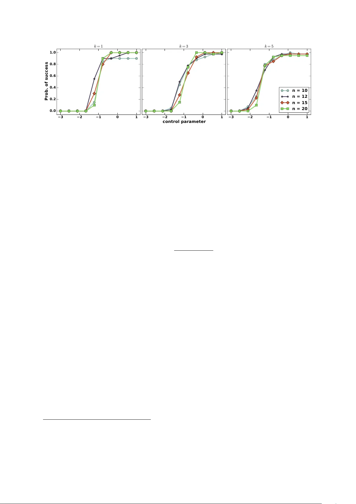
F rom Behavio r to Spa rse Graphical Games: Efficient Recovery of Equilib ria Asish Ghoshal and Jean Honorio Departmen t of Computer Science Purdue Univ ersit y W est Lafa y ette, IN - 47906 {aghoshal, jhonorio}@purdue.edu In this pap er w e study the problem of exact recov ery of the pure-strategy Nash equilibria (PSNE) set of a graphical game from noisy observ ations of joint actions of the pla y ers alone. W e consider sparse linear influence gam es — a parametric class of graphical games with linear pa yoffs, and represen ted by directed graphs of n nodes (pla yers) and in-degree of at most k . W e present an ` 1 -regularized logistic regression based algorithm for reco vering the PSNE set exactly , that is b oth computationally efficien t — i.e. runs in polynomial time — and statistically efficient — i.e. has logarithmic sample complexit y . Sp ecifically , w e sho w that the sufficien t n um b er of samples required for exact PSNE reco very scales as O (p oly( k ) log n ) . W e also v alidate our theoretical results using synthetic exp eriments. 1 Intro duction and Related W o rk Non-co op erativ e game theory is widely regarded as an appropriate mathematical framework for studying str ate gic b ehavior in m ulti-agent scenarios. The core solution concept of Nash e quilibrium describ es the stable outcome of the o verall b eha vior of self-interested agents — for instance p eople, companies, gov ernmen ts, groups or autonomous systems — in teracting strategically with each other and in distributed settings. Ov er the past few y ears, considerable progress has b een made in analyzing b eha vioral data using game-theoretic tools, e.g. computing Nash equilibria [1, 2, 3], most influen tial agen ts [4], price of anarch y [5] and related concepts in the context of graphical games. In p olitic al scienc e for instance, Irfan and Ortiz [4] identified, from congressional v oting records, the most influen tial senators in the U.S. congress — a small set of senators whose collectiv e b ehavior forces every other senator to a unique choice of vote. Irfan and Ortiz [4] also observed that the most influential senators w ere strikingly similar to the gang-of-six senators, formed during the national debt ceiling negotiations of 2011. F urther, using graphical games, Honorio and Ortiz [6] sho wed that Obama’s influence on Republicans increased in the last sessions b efore candidacy , while McCain’s influence on Republicans decreased. The problems in algorithmic game the ory described ab ov e, i.e. computing the Nash equilibria, computing the price of anarc hy or finding the most influen tial agen ts, require a kno wn graphical 1 game which is not av ailable apriori in real-world settings. Therefore, Honorio and Ortiz [6] prop osed learning graphical games from b ehavioral data, using maxim um likelihoo d estimation (MLE) and sp arsity -promoting metho ds. Honorio and Ortiz [6] and Irfan and Ortiz [4] hav e also demonstrated the usefulness of learning sp arse graphical games from b ehavioral data in real-w orld settings, through their analysis of the v oting records of the U.S. congress as well as the U.S. supreme court. In this pap er, we analyze a particular metho d prop osed by Honorio and Ortiz [6] for learning sparse linear influence games, namely , using logistic regression for learning the neighborho o d of each play er in the graphical game, indep endently . Honorio and Ortiz [6] show ed that the metho d of indep endent logistic regression is likelihoo d consisten t; i.e. in the infinite sample limit, the lik eliho o d estimate con verges to the true achiev able lik eliho o d. In this pap er w e obtain the stronger guarantee of recov ering the true PSNE set exactly . Needless to sa y , our stronger guaran tee comes with additional conditions that the true game m ust satisfy in order to allow for exact PSNE recov ery . The most crucial among our conditions is the assumption that the minim um pay off across all play ers and all join t actions in the true PSNE set is strictly p ositiv e. W e show, through sim ulation experiments, that our assumptions indeed b ears out for large classes of graphical games, where we are able to exactly reco ver the PSNE set. Finally , we w ould like to draw the attention of the reader to the fact that ` 1 -regularized logistic regression has b een analyzed b y Ravikumar et. al. [7] in the con text of learning sparse Ising mo dels. Apart from technical differences and differences in pro of techniques, our analysis of ` 1 -p enalized logistic regression for learning sparse graphical games differs from Ravikumar et. al. [7] conceptually — in the sense that we are not interested in reco vering the edges of the true game graph, but only the PSNE set. Therefore, we are able to av oid some stronger and non-in tuitive conditions required b y Ravikumar et. al. [7], such as m utual incoherence. The rest of the pap er is organized as follows. In section 2 w e provide a brief ov erview of graphical games and, sp ecifically , linear influence games. W e then formalize the problem of learning linear influence games in section 3. In section 4, w e presen t our main metho d and asso ciated theoretical results. Then, in section 5 we pro vide exp erimental v alidation of our theoretical guarantees. Finally , in section 6 we conclude b y discussing av en ues for future w ork. 2 Prelimina ries In this section w e review k ey concepts behind graphical games introduced b y Kearns et. al. [8] and linear influence games (LIGs) introduced by Irfan and Ortiz [4] and Honorio and Ortiz [6]. 2.1 Graphical Games A normal-form game G in classical game theory is defined by the triple G = ( V , A , U ) of play ers, actions and pay offs. V is the set of pla yers, and is given b y the set V = { 1 , . . . , n } , if there are n pla yers. A is the set of actions or pur e-str ate gies and is given by the Cartesian pro duct A . = × i ∈ V A i , where A i is the set of pure-strategies of the i -th play er. Finally , U . = { u i } n i =1 , is the set of pa y offs, where u i : A i × j ∈ V \ i A j → R sp ecifies the pa y off for the i -th pla y er giv en its action and the join t actions of the all the remaining pla y ers. A key solution concept in non-co op erativ e game theory is the Nash e quilibrium . F or a non- co op erativ e game, a joint action x ∗ ∈ A is a pure-strategy Nash equilibrium (PSNE) if, for eac h pla yer i , x ∗ i ∈ argmax x i ∈ A i u i ( x i , x ∗ − i ) , where x ∗ − i = { x ∗ j | j 6 = i } . In other w ords, x ∗ constitutes the mutual b est-resp onse for all play ers and no play er has any incentiv e to unilaterally deviate from their optimal action x ∗ i giv en the join t actions of the remaining pla yers x ∗ − i . The set of all 2 pur e-str ate gy Nash e quilibrium (PSNE) for a game G is defined as follo ws: N E ( G ) =  x ∗   ( ∀ i ∈ V ) x ∗ i ∈ argmax x i ∈ A i u i ( x i , x ∗ − i )  . (1) Gr aphic al games , introduced by Kearns et. al. [8], extend the formalism of Gr aphic al mo dels to games. That is, a graphical game G is defined by the dir e cte d gr aph , G = ( V , E ) , of vertices and directed edges (arcs), where v ertices corresp ond to pla yers and arcs enco de “influence” among pla yers i.e. the pay off of the i -th play er only dep ends on the actions of its (incoming) neigh b ors. 2.2 Linea r Influence Games Linear influence games (LIGs), introduced by Irfan and Ortiz [4] and Honorio and Ortiz [6], are graphical games with binary actions, or pure strategies, and parametric (linear) pay off functions. W e assume, without loss of generality , that the joint action space A = {− 1 , +1 } n . A linear influence game betw een n pla y ers, G ( n ) = ( W , b ) , is c haracterized b y (i) a matrix of w eigh ts W ∈ R n × n , where the en try W ij indicates the amount of influence (signed) that the j -th pla yer has on the i -th pla y er and (ii) a bias vector b ∈ R n , where b i captures the prior preference of the i -th play er for a particular action x i ∈ {− 1 , +1 } . The pa yoff of the i -th play er given the actions of the remaining play ers is then given as u i ( x i , x − i ) = x i ( w T − i x − i − b i ) , and the PSNE set is defined as follo ws: N E ( G ( n )) =  x | ( ∀ i ) x i ( w T − i x − i − b i ) ≥ 0  , (2) where w − i denotes the i -th row of W without the i -th entry , i.e. w − i = { w ij | j 6 = i } . Note that w e ha ve diag( W ) = 0 . F or linear influence games G ( n ) , we can define the neighborho o d and signed neigh b orho o d of the i -th vertex as N ( i ) = { j | | w i,j | > 0 } and N ± ( i ) = { sign( w ij ) | j ∈ N ( i ) } resp ectiv ely . It is imp ortan t to note that we don’t include the outgoing arcs in our definition of the neighborho o d of a vertex. Thus, for linear influence games, the w eight matrix W and the bias v ector b , completely sp ecify the game and the PSNE set induced by the game. Finally , let G ( n, k ) denote sparse games o v er n play ers where the in-degree of an y vertex is at most k , i.e. for all i , |N i | ≤ k . 3 Problem F o rmul ation Ha ving in tro duced the necessary definitions, w e no w in tro duce the problem of learning sparse linear influence games from observ ations of joint actions only . W e assume that there exists a game G ∗ ( n, k ) = ( W ∗ , b ∗ ) from which a “noisy” data set D = { x ( l ) } m l =1 of m observ ations is generated, where each observ ation x ( l ) is sampled independently and iden tically from the follo wing distribution: p ( x ) = q 1 [ x ∈ N E ∗ ] |N E ∗ | + (1 − q ) 1 [ x / ∈ N E ∗ ] 2 n − |N E ∗ | . (3) In the ab o ve distribution, q is the probability of observing a data p oint from the set of Nash equilibria and can b e though t of as the “signal” lev el in the data set, while 1 − q can b e though t of as the “noise” level in the data set. W e use N E ∗ instead of N E ( G ∗ ( n, k )) to simplify notation. W e further assume that the game is non-trivial 1 i.e. |N E ∗ | ∈ { 1 , . . . 2 n − 1 } and that q ∈ ( |N E ∗ | / 2 n , 1) . 1 This comes from Definition 4 in [6]. 3 The latter assumption ensures that the signal level in the data set is more than the noise lev el 2 . W e define the equality of t wo games G ∗ ( n, k ) = ( W ∗ , b ∗ ) and b G ( n, k ) = ( c W , b b ) as follows: G ∗ ( n, k ) = b G ( n, k ) iff ( ∀ i ) N ∗ ± ( i ) = b N ± ( i ) ∧ sign( b ∗ i ) = sign( b b i ) ∧ N E ∗ = d N E . A natural question to ask then is that, giv en only the data set D and no other information, is it p ossible to reco ver the w eigh t matrix c W and the bias v ector b b such that b G ( n, k ) = G ∗ ( n, k ) ? Honorio and Ortiz [6] show ed that it is in general imp ossible to learn the true game G ∗ ( n, k ) from observ ations of joint actions only b ecause m ultiple w eight matrices W and bias v ectors b can induce the same PSNE set and therefore hav e the same likelihoo d under the observ ation model (3) — an issue known as non-identifiablit y in the statistics literature. It is, how ever, p ossible to learn the equiv alence class of games that induce the same PSNE set. W e define the equiv alence of tw o games G ∗ ( n, k ) and b G ( n, k ) simply as : G ∗ ( n, k ) ≡ b G ( n, k ) iff N E ∗ = d N E . Therefore, our goal in this pap er is efficien t and consistent recov ery of the pure-strategy Nash equilibria set (PSNE) from observ ations of joint actions only; i.e. given a data set D , drawn from some game G ∗ ( n, k ) according to (3), w e infer a game b G ( n, k ) from D such that b G ( n, k ) ≡ G ∗ ( n, k ) . 4 Metho d and Results Our main metho d for learning the structure of a sparse LIG, G ∗ ( n, k ) , is based on using ` 1 - regularized logistic regression, to learn the parameters ( w − i , b i ) for eac h play er i indep enden tly . W e denote by v i ( W , b ) = ( w − i , − b i ) the parameter v ector for the i -th play er, which character- izes its pay off; and b y z i ( x ) = ( x i x − i , x i ) the “feature” v ector. In the rest of the pap er w e use v i and z i instead of v i ( W , b ) and z i ( x ) resp ectively , to simplify notation. Then, we learn the parameters for the i -th pla yer as follo ws: b v i = argmin v i ` ( v i , D ) + λ k v i k 1 (4) ` ( v i , D ) = 1 m m X l =1 log(1 + exp( − v T i z ( l ) i )) . (5) W e then set b w − i = [ b v i ] 1:( n − 1) and b b i = − [ b v i ] n , where the notation [ . ] i : j denotes indices i to j of the vector. W e sho w that, under suitable assumptions on the true game G ∗ ( n, k ) = ( W ∗ , b ∗ ) , the parameters c W and b b obtained using (5) induce the same PSNE set as the true game, i.e. N E ( W ∗ , b ∗ ) = N E ( c W , b b ) . Before presen ting our main results, ho wev er, w e state and discuss the assumptions on the true game under whic h it is p ossible to reco ver the true PSNE set of the game using our proposed metho d. 4.1 Assumptions The success of our metho d hinges on certain assumptions on the structure of the underlying game. These assumptions are in addition to the assumptions imp osed on the parameter q and the num b er of Nash equilibria of the game |N E ∗ | , as required by definition of a LIG. Since the 2 See Prop osition 5 and Definition 7 in [6] for a justification of this. 4 assumptions are related to the Hessian of the loss function (5), w e take a moment to introduce the expressions of the gradient and the Hessian here. The gradient and Hessian of the loss function for any v ector v and the data set D is given as follows: ∇ ` ( v , D ) = 1 m m X l =1 ( − z ( l ) 1 + exp( v T z ( l ) ) ) (6) ∇ 2 ` ( v , D ) = 1 m m X l =1 η ( v T z ( l ) ) z ( l ) z ( l ) T , (7) where η ( x ) = 1 / ( e x/ 2 + e − x/ 2 ) 2 . Finally , H m i denotes the sample Hessian matrix with resp ect to the i -th play er and the true parameter v ∗ i , and H ∗ i denotes it’s exp ected v alue, i.e. H ∗ i . = E D [ H m i ] = E D  ∇ 2 ` ( v ∗ i , D )  . In subsequen t sections w e drop the notational dep endence of H ∗ i and z i on i to simplify notation. How ever, it should b e noted that the assumptions are with resp ect to each pla yer and m ust hold individually for eac h play er i . Now we are ready to state and describ e the implications of our assumptions. The following assumption ensures that the exp ected loss is strongly conv ex and smo oth. Assumption 1. L et S b e the supp ort of the ve ctor v , i.e. S . = { i | | v i | > 0 } . Then, ther e exists c onstants C min > 0 and D max ≤ | S | such that: λ min ( H ∗ S S ) ≥ C min and λ max ( E x  z S z T S  ) ≤ D max , for al l i , wher e λ min ( . ) and λ max ( . ) denote the minimum and maximum eigenvalues r esp e ctively and H ∗ S S = { H ∗ i,j | i, j ∈ S } . T o b etter understand the implications of the ab o ve assumptions first note that the distribution o ver joint actions in (3), after some algebraic manipulations, can be written as follows: p ( x ) =  q − |N E ∗ | / 2 n 1 − |N E ∗ | / 2 n  1 [ x ∈ N E ∗ ] |N E ∗ |  1 − q 1 − |N E ∗ | / 2 n  1 2 n . (8) Th us, we ha ve that the distribution o ver joint actions is a mixture of t wo uniform distributions, one ov er the n umber of Nash equilibria and the other b eing the Rademacher distribution ov er n v ariables. W e denote the latter distribution by R n , i.e. x ∼ R n = ⇒ x ∈ {− 1 , +1 } n ∧ p ( x ) = 1 / 2 n for all x . Therefore the exp ected Hessian matrix H ∗ decomp oses as a conv ex combination of t wo other Hessian matrices: H ∗ = ν H N E ∗ + (1 − ν ) H R , (9) where we hav e defined: H N E ∗ . = 1 |N E ∗ | X x ∈N E ∗ η ( v ∗ T z ) zz T , H R . = E z ∼ R n h η ( v ∗ T z ) zz T i , ν . =  q − |N E ∗ | / 2 n 1 − |N E ∗ | / 2 n  . No w, by conca vity of λ min ( . ) and the Jensen’s inequalit y we ha ve that C min ≥ ν λ min ( H N E ∗ S S ) + (1 − ν ) λ min ( H R S S ) ≥ ν λ min ( H N E ∗ S S ) + (1 − ν ) η ( k v ∗ k 1 ) ≥ (1 − ν ) η ( k v ∗ k 1 ) > 0 , 5 where the last line follo ws from the fact that H N E ∗ S S is p ositive semi-definite. In fact the minimum eigen v alue, λ min ( H N E ∗ S S ) , is zero if |N E ∗ | < n . Thus, we hav e that our assumption of q ∈ ( N E ∗ / 2 n , 1) automatically implies that λ min ( H ∗ i ) ≥ C min > 0 . W e can also v erify that the maxim um eigenv alue is b ounded as follo ws: D max ≤ ν λ max 1 |N E ∗ | X x ∈N E ∗ z S z T S ! + (1 − ν ) λ max ( E z ∼ R n  z S z T S  ) ≤ ν | S | + (1 − ν ) . The following assumption c haracterizes the minimum pay off in the Nash equilibria set. Assumption 2. The minimum p ayoff in the PSNE set, ρ min , is strictly p ositive, sp e cific al ly: x i ( w ∗ − i T x − i − b i ) ≥ ρ min > 5 C min / D max ( ∀ x ∈ N E ∗ ) . Note that as long as the minimum pay off is strictly p ositive, we can scale the parameters ( W ∗ , b ∗ ) by the constan t 5 C min / D max to satisfy the condition: ρ min > 5 C min / D max , without chang- ing the PSNE set or the likelihoo d of the data. Indeed the assumption that the minimum pa yoff is strictly p ositiv e is is una voidable for exact recov ery of the PSNE set in a noisy setting suc h as ours, b ecause otherwise this is akin to exactly recov ering the parameters v for eac h pla yer i . F or example, if x ∈ N E ∗ is suc h that v ∗ T x = 0 , then it can b e shown that ev en if k v ∗ − b v k ∞ = ε , for any ε arbitrarily close to 0 , then b v T x < 0 and therefore N E ( W ∗ , b ∗ ) 6 = N E ( c W , b b ) . Next, w e present our main theoretical results for learning LIGs. 4.2 Theo retical Guarantees Our main strategy for obtaining exact PSNE reco v ery guaran tees is to first show, using results from random matrix theory , that giv en the assumptions on the eigenv alues of the p opulation Hessian matrices, the assumptions hold in the finite sample case with high probability . Then, w e exploit the conv exity prop erties of the logistic loss function to sho w that the weigh t v ectors learned using p enalized logistic regression is “close” to the true weigh t vectors. By our assumption that the minim um pay off in the PSNE set is strictly greater than zero, we show that the weigh t v ectors inferred from a finite sample of join t actions induce the same PSNE set as the true weigh t v ectors. 4.2.1 Minimum and Maximum Eigenvalues of Finite Sample Hessian and Scatter Matrices The following tec hnical lemma shows that the assumptions on the eigenv alues of the Hessian matrices, hold with high probabilit y in the finite sample case. Lemma 1. If λ min ( H ∗ S S ) ≥ C min and λ max ( E x  z S z T S  ) ≤ D max then we have that λ min ( H m S S ) ≥ C min 2 and λ max m X l =1 z ( l ) S z ( l ) S T ! ≤ 2 D max with pr ob ability at le ast 1 − | S | exp  − mC min 2 | S |  and 1 − | S | exp  − m (1 − ν ) 4 | S |  r esp e ctively. 6 Pr o of. Let µ min . = λ min ( H ∗ S S ) and µ max . = λ max ( E x  z S z T S  ) . First note that for all z ∈ {− 1 , +1 } n : λ max ( η ( v ∗ S T z S ) z S z T S ) ≤ | S | 4 . = R λ max ( z S z T S ) ≤ | S | . = R 0 . Using the Matrix Chernoff b ounds from T ropp [9](Theorem 1.1), w e hav e that Pr { λ min ( H m S S ) ≤ (1 − δ ) µ min } ≤ | S |  e − δ (1 − δ ) 1 − δ  mµ min R . Setting δ = 1 / 2 we get that Pr { λ min ( H m S S ) ≤ µ min / 2 } ≤ | S | " r 2 e # 4 mµ min | S | ≤ | S | exp  − mC min 2 | S |  . Therefore, we hav e Pr { λ min ( H m S S ) > C min / 2 } > 1 − | S | exp  − mC min 2 | S |  . Next, we hav e that µ max = λ max ( E x  z S z T S  ) ≥ λ min ( E x  z S z T S  ) ≥ ν λ min 1 |N E ∗ | X x ∈N E ∗ z S z T S ! + (1 − ν ) ≥ (1 − ν ) . Once again inv oking Theorem 1.1 from [9] and setting δ = 1 we ha ve that Pr { λ max ≥ (1 + δ ) µ max } ≤ | S |  e δ (1 + δ ) 1+ δ  ( mµ max ) / R 0 = ⇒ Pr { λ max ≥ 2 µ max } ≤ | S | h e 4 i ( mµ max ) / | S | ≤ | S | exp  − mµ max 4 | S |  ≤ | S | exp  − m (1 − ν ) 4 | S |  . Therefore, we hav e that Pr { λ max < 2 D max } > 1 − | S | exp  − m (1 − ν ) 4 | S |  . 4.2.2 Recovering the Pure Strategy Nash Equilibria (PSNE) Set Before presen ting our main result on the exact recov ery of the PSNE set from noisy observ ations of join t actions, we first presen t a few technical lemmas that w ould b e helpful in pro ving the main result. The following lemma b ounds the gradient of the loss function (5) at the true vector v ∗ , for all pla y ers. 7 Lemma 2. With pr ob ability at le ast 1 − δ for δ ∈ [0 , 1] , we have that k∇ ` ( v ∗ , D ) k ∞ < ν κ + r 2 m log 2 n δ , wher e κ = 1 / (1+exp( ρ min )) and ρ min ≥ 0 is the minimum p ayoff in the PSNE set. Pr o of. Let u m . = ∇ ` ( v ∗ , D ) and u m j denote the j -th index of u m . W e ha ve that ( ∀ j ∈ S c ∧ j 6 = n ) E  u m j  = ν |N E ∗ | X x ∈N E ∗ z j 1 + exp(( v ∗ S ) T z S ) + (1 − ν ) E z ∼ R n  z j 1 + exp(( v ∗ S ) T z S )  = ν |N E ∗ | X x ∈N E ∗ z j 1 + exp(( v ∗ S ) T z S ) + (1 − ν )  E z S ∼ R | S |  1 1 + exp(( v ∗ S ) T z S )  E z j ∼ R [ z j ]  ≤ ν κ |N E ∗ | X x ∈N E ∗ x i x j ≤ ν κ Similarly , ( ∀ j ∈ S ∧ j 6 = n ) E  u m j  = ν |N E ∗ | X x ∈N E ∗ z j 1 + exp(( v ∗ S ) T z S ) + (1 − ν ) E z ∼ R n  z j 1 + exp(( v ∗ S ) T z S )  ≤ ν |N E ∗ | X x ∈N E ∗ z j 1 + exp(( v ∗ S ) T z S ) + (1 − ν ) E z j ∼ R [ z j ] ≤ ν κ. F ollowing the same pro cedure as ab o ve, it can b e easily shown that the ab ov e b ounds hold for the case j = n as w ell. Also note that    u m j    ≤ 1 . Therefore, b y using the Ho effding’s inequalit y [10] and a union b ound argument we ha ve that: Pr  n max j =1   u m j − E  u m j    < t  > 1 − 2 ne − mt 2 / 2 = ⇒ Pr {k u m − E [ u m ] k ∞ < t } > 1 − 2 ne − mt 2 / 2 = ⇒ Pr {k u m k ∞ − k E [ u m ] k ∞ < t } > 1 − 2 ne − mt 2 / 2 = ⇒ Pr {k u m k ∞ < ν κ + t } > 1 − 2 ne − mt 2 / 2 . Setting 2 n exp( − mt 2 / 2 ) = δ , w e prov e our claim. A consequence of Lemma 2 is that, ev en with an infinite num b er of samples, the gradient of the loss function at the true vector v ∗ do esn’t v anish. Therefore, we cannot hop e to recov er the parameters of the true game p erfectly even with an infinite num b er of samples. In the follo wing technical lemma we show that the optimal vector b v for the logistic regression problem is close to the true v ector v ∗ in the supp ort set S of v ∗ . Next, in Lemma 4, we b ound the difference b etw een the true v ector v ∗ and the optimal vector b v in the non-supp ort set. The lemmas together show that the optimal v ector is close to the true vector. 8 Lemma 3. If the r e gularization p ar ameter λ satisfies the fol lowing c ondition: λ ≤ 5 C 2 min 16 | S | D max − ν κ − r 2 m log 2 n δ , then k v ∗ S − b v S k 2 ≤ 5 C min 4 p | S | D max , with pr ob ability at le ast 1 − ( δ + | S | exp( ( − mC min ) / 2 | S | ) + | S | exp( ( − m (1 − ν )) / 4 | S | )) . Pr o of. The pro of of this lemma follows the general pro of structure of Lemma 3 in [7]. First, we reparameterize the ` 1 -regularized loss function f ( v S ) = ` ( v S ) + λ k v S k 1 as the loss function e f , which giv es the loss at a p oin t that is ∆ S distance aw a y from the true parameter v ∗ S as follows: e f (∆ S ) = ` ( v ∗ S + ∆ S ) − ` ( v ∗ S ) + λ ( k v ∗ S + ∆ S k 1 − k v ∗ S k 1 ) , where ∆ S = v S − v ∗ S . Also note that the loss function e f is shifted such that the loss at the true parameter v ∗ S is 0 , i.e. e f ( 0 ) = 0 . F urther, note that the function e f is con vex and is minimized at b ∆ S = b v S − v ∗ S , since b v S minimizes f . Therefore, clearly e f ( b ∆ S ) ≤ 0 . Thus, if we can show that the function e f is strictly p ositiv e on the surface of a ball of radius b , then the p oint b ∆ S lies inside the ball i.e. k b v S − v ∗ S k 2 ≤ b . Using the T aylor’s theorem w e expand the first term of e f to get the follo wing: e f (∆ S ) = ∇ ` ( v ∗ S ) T ∆ S + ∆ T S ∇ 2 ` ( v ∗ S + θ ∆ S )∆ S + λ ( k v ∗ S + ∆ S k 1 − k v ∗ S k 1 ) , (10) for some θ ∈ [0 , 1] . Next, we low er b ound each of the terms in (10). Using the Cauch y-Sc hw artz inequalit y , the first term in (10) is b ounded as follo ws: ∇ ` ( v ∗ S ) T ∆ S ≥ − k∇ ` ( v ∗ S ) k ∞ k ∆ S k 1 ≥ − k∇ ` ( v ∗ S ) k ∞ p | S | k ∆ S k 2 ≥ − b p | S | ν κ + r 2 m log 2 n δ ! , (11) with probability at least 1 − δ for δ ∈ [0 , 1] . It is also easy to upp er b ound the last term in equation 10, using the rev erse triangle inequalit y as follows: λ |k v ∗ S + ∆ S k 1 − k v ∗ S k 1 | ≤ λ k ∆ S k 1 . Whic h then implies the following low er b ound: λ ( k v ∗ S + ∆ S k 1 − k v ∗ S k 1 ) ≥ − λ k ∆ S k 1 ≥ − λ p | S | k ∆ S k 2 = − λ p | S | b. (12) No w we turn our atten tion to computing a lo wer b ound of the second term of (10), which is a bit more inv olv ed. ∆ T S ∇ 2 ` ( v ∗ S + θ ∆ S )∆ S ≥ min k ∆ S k 2 = b ∆ T S ∇ 2 ` ( v ∗ S + θ ∆ S )∆ S = b 2 λ min ( ∇ 2 ` ( v ∗ S + θ ∆ S )) . 9 No w, λ min ( ∇ 2 ` ( v ∗ S + θ ∆ S )) ≥ min θ ∈ [0 , 1] λ min  ∇ 2 ` ( v ∗ S + θ ∆ S )  = min θ ∈ [0 , 1] λ min 1 m m X l =1 η (( v ∗ S + θ ∆ S ) T z ( l ) S ) z ( l ) S ( z ( l ) S ) T ! . Again, using the T aylor’s theorem to expand the function η we get η (( v ∗ S + θ ∆ S ) T z ( l ) S ) = η (( v ∗ S ) T z ( l ) S ) + η 0 (( v ∗ S + ¯ θ ∆ S ) T z ( l ) S )( θ ∆ S ) T z ( l ) S , where ¯ θ ∈ [0 , θ ] . Contin uing from ab ov e and from Lemma 1 we hav e, with probabilit y at least 1 − | S | exp( ( − mC min ) / 2 | S | ) : λ min  ∇ 2 ` ( v ∗ S + θ ∆ S )  ≥ min θ ∈ [0 , 1] λ min 1 m m X l =1 η (( v ∗ S ) T z ( l ) S ) z ( l ) S ( z ( l ) S ) T + 1 m m X l =1 η 0 (( v ∗ S + ¯ θ ∆ S ) T z ( l ) S )(( θ ∆ S ) T z ( l ) S ) z ( l ) S ( z ( l ) S ) T ! ≥ λ min ( H m S S ) − max θ ∈ [0 , 1] | | | A ( θ ) | | | 2 ≥ C min 2 − max θ ∈ [0 , 1] | | | A ( θ ) | | | 2 , where we hav e defined A ( θ ) . = 1 m m X l =1 η 0 (( v ∗ S + θ ∆ S ) T z ( l ) S )( θ ∆ S ) T z ( l ) S z ( l ) S ( z ( l ) S ) T . Next, the sp ectral norm of A ( θ ) can b e b ounded as follo ws: | | | A ( θ ) | | | 2 ≤ max k y k 2 =1 ( 1 m m X l =1    η 0 (( v ∗ S + θ ∆ S ) T z ( l ) S )       (( θ ∆ S ) T z ( l ) S )    × y T ( z ( l ) S ( z ( l ) S ) T ) y ) < max k y k 2 =1 ( 1 10 m m X l =1 k ( θ ∆ S ) k 1    z ( l ) S    ∞ y T ( z ( l ) S ( z ( l ) S ) T ) y ) ≤ θ max k y k 2 =1 ( 1 10 m m X l =1 p | S | k ∆ S k 2 y T ( z ( l ) S ( z ( l ) S ) T ) y ) = θ b p | S |                1 10 m m X l =1 z ( l ) S ( z ( l ) S ) T                2 ≤ ( b p | S | D max ) 5 ≤ C min 4 , where in the second line we used the fact that η 0 ( . ) < 1 / 10 and in the last line w e assumed that ( b √ | S | D max ) / 5 ≤ C min / 4 — an assumption that we verify momentarily . Ha ving upp er b ounded the sp ectral norm of A ( θ ) , w e hav e λ min  ∇ 2 ` ( v ∗ S + θ ∆ S )  ≥ C min 4 . (13) 10 Plugging back the bounds giv en by (11), (12) and (13) in (10) and equating to zero we get − b p | S | ν κ + r 2 m log 2 n δ ! + b 2 C min 4 − λ p | S | b = 0 = ⇒ b = 4 p | S | C min λ + ν κ + r 2 m log 2 n δ ! . Finally , coming back to our prior assumption we hav e b = 4 p | S | C min λ + ν κ + r 2 m log 2 n δ ! ≤ 5 C min 4 p | S | D max . The ab ov e assumption holds if the regularization parameter λ is b ounded as follows: λ ≤ 5 C 2 min 16 | S | D max − r 2 m log 2 n δ − ν κ. Lemma 4. If the r e gularization p ar ameter λ satisfies the fol lowing c ondition: λ ≥ ν κ + r 2 m log 2 n δ , then we have that k b v − v ∗ k 1 ≤ 5 C min D max with pr ob ability at le ast 1 − ( δ + | S | exp( ( − mC min ) / 2 | S | ) + | S | exp( ( − m (1 − ν )) / 4 | S | )) . Pr o of. Define ∆ . = b v − v ∗ . Also for any vector y let the notation y S denote the vector y with the entries not in the supp ort, S , set to zero, i.e.  y S  i =  y i if i ∈ S , 0 otherwise . Similarly , let the notation y S c denote the vector y with the entries not in S c set to zero, where S c is the complement of S . Having introduced our notation and since, S is the supp ort of the true v ector v ∗ , we hav e by definition that v ∗ = v ∗ S . W e then hav e, using the rev erse triangle inequalit y , k b v k 1 = k v ∗ + ∆ k 1 =   v ∗ S + ∆ S + ∆ S c   1 =   v ∗ S − ( − ∆ S )   1 +   ∆ S c   1 ≥ k v ∗ k 1 −   ∆ S   1 +   ∆ S c   1 . (14) Also, from the optimalit y of b v for the ` 1 -regularized problem we ha ve that ` ( v ∗ ) + λ k v ∗ k 1 ≥ ` ( b v ) + λ k b v k 1 = ⇒ λ ( k v ∗ k 1 − k b v k 1 ) ≥ ` ( b v ) − ` ( v ∗ ) . (15) 11 Next, from conv exit y of ` ( . ) and using the Cauc h y-Sch wartz inequality w e hav e that ` ( b v ) − ` ( v ∗ ) ≥ ∇ ` ( v ∗ ) T ( b v − v ∗ ) ≥ − k∇ ` ( v ∗ ) k ∞ k ∆ k 1 ≥ − λ 2 k ∆ k 1 , (16) where in the last line w e used the fact that λ ≥ k∇ ` ( v ∗ ) k ∞ . Thus, we hav e from (14), (15) and (16) that 1 2 k ∆ k 1 ≥ k b v k 1 − k v ∗ k 1 = ⇒ 1 2 k ∆ k 1 ≥   ∆ S c   1 −   ∆ S   1 = ⇒ 1 2   ∆ S c   1 + 1 2   ∆ S   1 ≥   ∆ S c   1 −   ∆ S   1 = ⇒ 3   ∆ S   1 ≥   ∆ S c   1 . (17) Finally , from (17) and Lemma 3 w e hav e that k ∆ k 1 =   ∆ S   1 +   ∆ S c   1 ≤ 4   ∆ S   1 ≤ 4 p | S |   ∆ S   2 ≤ 5 C min D max . No w we are ready to presen t our main result on recov ering the true PSNE set. Theorem 1. If for al l i , | S i | ≤ k , the minimum p ayoff ρ min ≥ 5 C min / D max , and the r e gularization p ar ameter and the numb er of samples satisfy the fol lowing c onditions: ν κ + r 2 m log 6 n 2 δ ≤ λ ≤ 2 K + ν κ − r 2 m log 6 n 2 δ (18) m ≥ max ( 2 K 2 log  6 n 2 δ  , 2 k C min log  3 k n δ  , 4 k 1 − ν log  3 k n δ  ) , (19) wher e K . = 5 C 2 min / 32 k D max − ν κ , then with pr ob ability at le ast 1 − δ , for δ ∈ [0 , 1] , we r e c over the true PSNE set, i.e. N E ( c W , b b ) = N E ( W ∗ , b ∗ ) . Pr o of. F rom Cauch y-Sc hw artz inequalit y and Lemma 4 w e hav e   ( b v i − v ∗ i ) T z i   ≤ k b v i − v ∗ i k 1 k z i k ∞ ≤ 5 C min D max . Therefore, we hav e that ( v ∗ i ) T z i − 5 C min D max ≤ b v T i z i ≤ ( v ∗ i ) T z i + 5 C min D max . No w, if ∀ x ∈ N E ∗ , ( v ∗ i ) T z i ≥ 5 C min / D max , then b v T i z i ≥ 0 . Using an union b ound argumen t ov er all play ers i , w e can sho w that the abov e holds with probabilit y at least 1 − n ( δ + k exp( ( − mC min ) / 2 k ) + k exp( ( − m (1 − ν )) / 4 k )) (20) for all pla y ers. Therefore, we hav e that N E ( c W , b b ) = N E ∗ with high probabilit y . Finally , setting δ = δ 0 / 3 n , for some δ 0 ∈ [0 , 1] , and ensuring that the last tw o terms in (20) are at most δ 0 / 3 n eac h, w e prov e our claim. 12 T o better understand the implications of the theorem ab ov e, w e discuss some p ossible op er- ating regimes for learning sparse linear influence games in the following paragraphs. Remark 1 (Sample complexity for fixed q ) . In the the or em ab ove, if q is c onstant, which in turn makes ν c onstant, then K = Ω ( 1 / k 2 ) , and the sample c omplexity of le arning sp arse line ar games gr ows as O  k 4 log n  . However, if q is smal l enough such that ν ≤ 1 / k , then the c onstant D max is no longer a function of k and henc e K = Ω ( 1 / k ) . Ther efor e, the sample c omplexity sc ales as O  k 2 log n  for exact PSNE r e c overy. The sample complexit y of O (p oly( k ) log n ) for exact reco very of the PSNE set can be com- pared with the sample complexit y of O  k n 3 log 2 n  for the maxim um lik eliho o d estimate (MLE) of the PSNE set as obtained by Honorio [11]. Note that while the MLE pro cedure is consistent, i.e. MLE of the PSNE set is equal to the true PSNE set with probabilit y con verging to 1 as the n umber of samples tend to infinity , it is NP-hard 3 . In contrast, the logistic regression metho d is computationally efficient. F urther, while the sample complexit y of our metho d seems to b e b etter than the empirical log-likelihoo d minimizer as given by Theorem 3 in [11], in this pap er w e restrict ourselves to LIGs with strictly p ositive pa y off in the PSNE set — such games are in v ariably easier to learn than general LIGs considered by [11]. Honorio [11] also obtained low er b ounds on the n umber of samples required b y any conceiv able metho d, for exact PSNE reco v ery , by scaling the parameter q with the n um b er of pla y ers. Therefore, in order to compare our results with the information-theoretic limits of learning LIGs, we consider the regime where the parameter q scales with the num b er of pla yers n . Remark 2 (Sample complexit y for q v arying with num b er of pla yers) . If we c onsider the r e gime wher e the signal level sc ales as q = ( |N E ∗ | +1) / 2 n . Then, D max = O ( k / (2 n −|N E ∗ | ) ) , and as a r esult K = Ω ( 2 n / k 2 ) . Ther efor e, the sample c omplexity, which is dominate d by the se c ond and thir d terms in (19) , is given as O ( k log ( k n )) . In gener al if q = Θ (exp( − n )) , then the sample c omplexity for r e c overing the PSNE set exactly is O ( k log( k n )) . Once again w e observ e that even in the regime of q scaling exp onentially with n , the sample complexit y of O ( k log( k n )) is b etter than the information theoretic limit of O  k n log 2 n  , b y a factor of O ( n log n ) . This can b e attributed to the fact that w e consider restricted ensembles of games with strictly positive pa yoffs in the PSNE set, as opposed to general LIGs. F urther, from the aforementioned remarks we see that as the signal level q decreases, the sufficien t num b er of samples needed to recov er the PSNE set reduces; and in the limiting case of q decreasing exp onen tially with the n umber of play ers, the sample complexit y scales as O ( k log( k n )) . This seems counter-in tuitive — with increased signal level, a learning problem should b ecome easier and not harder. T o understand this seemingly counter-in tuitiv e b ehavior, first observ e that the constant D max / C min can b e though t of as the “condition n umber” of the loss function given by 5, Therefore, the sample complexit y as given by Theorem 1 can b e written as O  k 2 ( D max / C min ) 2 log n  . F rom (9), we see that as the signal lev el increases, the Hessian of the loss b ecomes more ill-conditioned, since the data set now comprises of many repetitions of the few joint-actions that are in the PSNE set; thereb y increasing the dep endency ( D max ) b etw een actions of play ers in the sample data set. 13 −3 −2 −1 0 1 0.0 0.2 0.4 0.6 0.8 1.0 Prob. of success k = 1 −3 −2 −1 0 1 control parameter k = 3 −3 −2 −1 0 1 k = 5 n = 10 n = 12 n = 15 n = 20 Figure 1: The probability of exact reco very of the PSNE set computed across 40 randomly sampled LIGs as the n umber of samples is scaled as b ( C )(10 c )( k 2 log( 6 n 2 / δ )) c , where c is the control parameter and the constant C is 10000 for the k = 1 case and 1000 for the remaining tw o case. 5 Exp eriments In order to verify that our results and assumptions indeed hold in practice, w e p erformed v arious sim ulation experiments. W e generated random LIGs for n play ers and exactly k neighbors b y first creating a matrix W of all zeros and then setting k off-diagonal en tries of eac h row, chosen uniformly at random, to − 1 . W e set the bias for all pla y ers to 0 . W e found that any o dd v alue of k pro duces games with strictly p ositive pay off in the PSNE set. Therefore, for each v alue of k in { 1 , 3 , 5 } , and n in { 10 , 12 , 15 , 20 } , w e generated 40 random LIGs. The parameters q and δ were set to the constant v alue of 0 . 01 and the regularization parameter λ w as set according to Theorem 1 as some constan t multiple of p ( 2 / m ) log ( 2 n / δ ) . Figure 1 shows the probabilit y of successful recov ery of the PSNE, for v arious com binations of ( n, k ) , where the probability w as computed as the fraction of the 40 randomly sampled LIGs for which the learned PSNE set matc hed the true PSNE set exactly . F or each exp eriment, the num b er of samples w as computed as: b ( C )(10 c )( k 2 log( 6 n 2 / δ )) c , where c is the control parameter and the constant C is 10000 for k = 1 and 1000 for k = 3 and 5 . Th us, from Figure 1 we see that, the sample complexity of O  k 2 log n  as giv en by Theorem 1 indeed holds in practice — i.e. there exists constants c and c 0 suc h that if the num b er of samples is less than ck 2 log n , we fail to recov er the PSNE set exactly with high probabilit y , while if the n umber of samples is greater than c 0 k 2 log n then w e are able to reco ver the PSNE set exactly , with high probability . F urther, the scaling remains consisten t as the n umber of pla y ers n is c hanged from 10 to 20 . 6 Conclusion In this pap er, w e presented a computationally efficien t and statistically consisten t metho d, based on ` 1 -regularized logistic regression, for learning linear influence games — a sub class of parametric graphical games with linear pa y offs. Under some mild conditions on the true game, w e show ed that as long as the n umber of samples scales as O (p oly ( k ) log n ) , where n is the n umber of pla yers and k is the maxim um n um b er of neighbors of any play er; then w e can reco ver the pure-strategy Nash equilibria set of the true game in polynomial time and with 3 Irfan and Ortiz [4] sho wed that counting the n umber of Nash equilibria is # P-complete. Therefore, computing the log-likelihoo d is NP-hard. 14 probabilit y conv erging to 1 as the n umber of samples tend to infinit y . An in teresting direction for future work would be to consider structured actions — for instance p ermutations, directed spanning trees, directed acyclic graphs among others — thereb y extending the formalism of linear influence games to the structured prediction setting. A more tec hnical extension would b e to consider a lo cal noise mo del where the observ ations are dra wn from the PSNE set but with each action indep endently corrupted by some noise. Other ideas that migh t b e w orth pursuing are: considering mixed strategies, correlated equilibria and epsilon Nash equilibria, and incorp orating latent or unobserved actions and v ariables in the mo del. References [1] B. Blum, C. R. Shelton, and D. Koller, “A con tinuation metho d for nash equilibria in structured games,” Journal of Artificial Intel ligenc e R ese ar ch , vol. 25, pp. 457–502, 2006. [2] L. E. Ortiz and M. Kearns, “Nash propagation for lo op y graphical games,” in A dvanc es in Neur al Information Pr o c essing Systems , 2002, pp. 793–800. [3] D. Vickrey and D. Koller, “Multi-agen t algorithms for solving graphical games,” in AAAI/IAAI , 2002, pp. 345–351. [4] M. T. Irfan and L. E. Ortiz, “On influence, stable b ehavior, and the most influen tial individ- uals in net w orks: A game-theoretic approac h,” Artificial Intel ligenc e , vol. 215, pp. 79–119, 2014. [5] O. Ben-Zwi and A. Ronen, “Local and global price of anarc hy of graphical games,” The o- r etic al Computer Scienc e , vol. 412, no. 12, pp. 1196–1207, 2011. [6] J. Honorio and L. Ortiz, “Learning the structure and parameters of large-p opulation graph- ical games from b ehavioral data,” Journal of Machine L e arning R ese ar ch , vol. 16, pp. 1157– 1210, 2015. [7] P . Ravikumar, M. W ain wright, and J. Lafferty , “ High-dimensional Ising mo del selection using L1-regularized logistic regression,” The Annals of Statistics , vol. 38, no. 3, pp. 1287–1319, 2010. [Online]. A v ailable: [8] M. Kearns, M. L. Littman, and S. Singh, “Graphical mo dels for game theory ,” in Pr o c e e dings of the Sevente enth c onfer enc e on Unc ertainty in Artificial Intel ligenc e . Morgan Kaufmann Publishers Inc., 2001, pp. 253–260. [9] J. A. T ropp, “User-friendly tail b ounds for sums of random matrices,” F oundations of c om- putational mathematics , vol. 12, no. 4, pp. 389–434, 2012. [10] W. Ho effding, “Probabilit y inequalities for sums of b ounded random v ariables,” Journal of the A meric an statistic al asso ciation , v ol. 58, no. 301, pp. 13–30, 1963. [11] J. Honorio, “ On the Sample Complexity of Learning Sparse Graphical Games,” 2016. [Online]. A v ailable: 15