Full-field Fourier ptychography (FFP): spatially varying pupil modeling and its application for rapid field-dependent aberration metrology

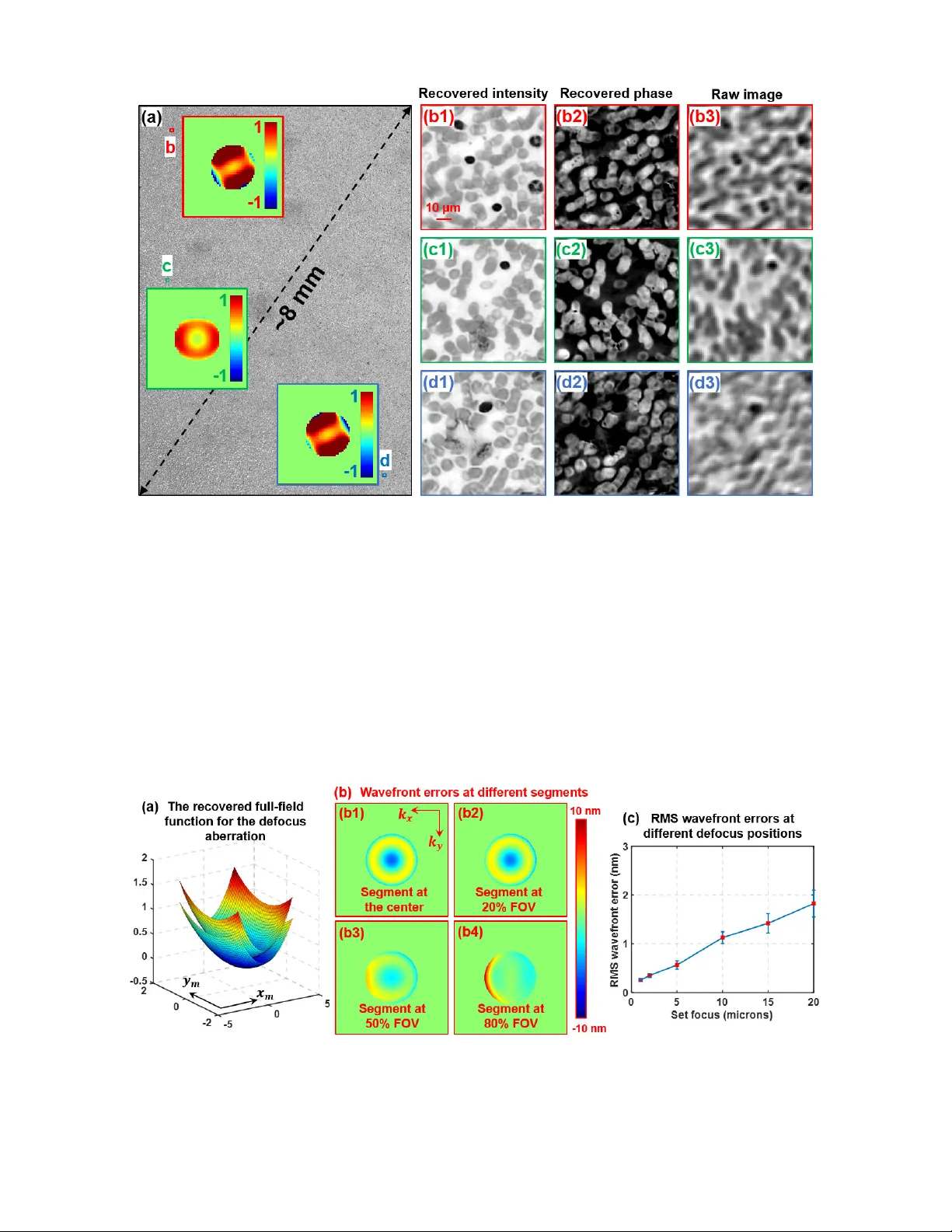
____________ ____________ ___ a) P. Song and S. Jiang contributed equally to this work b) Author to whom correspondence should be addressed. Email: guoan.zheng@uconn.edu. Full-field Fourier pty chography (FFP): spatially varying pupil modeling an d its application for rapid field-dependent aberration metrology Pengming Son g, 1,a) Shaowei Jiang, 2,a) He Zhang, 2 Xizhi Huang, 2,3 Yongbing Zhang, 3 and Guoan Zheng 1,2,b) 1 Department of Electrical and Computer Engine ering, University of Conn ecticut, Storrs, Connecti cut, 06269, USA 2 Department of Biomedical En gineering, University of Conn ecticut, Storrs, Conn ecticut, 06269, USA 3 Shenzhen Key Lab of Broadb and Network and Multimedia , Graduate School at Shenz hen, Tsinghua University, Shenzhen, Guangdong, 518055 , China Abstract : Digital aberration measurement and removal play a prominen t role in computational imaging platforms aimed at achieving simple and compact optical arrange ments. A recent important class of such platforms is Fourier ptychography, which is geared towards efficiently creating gigapixel images with high resolution and large field of view (FOV). In current FP implement ations, pupil a berration is often recovered at each sm all segm e nt of the entire FOV. This reconstruction strategy fails to consider the field-dependent nature of the optical pupil. Given the power series expansion of the wavefront aberration, the spatially varyi ng pupil can be fully characterized by ten s of coefficients ov er the entire FO V. With this observat ion, we report a Full-field Fo urier Ptychogr aphy (FFP) schem e for rapid and robust aberr ation metrology . The meaning of ‘full-field’ in FFP is referred to the recovering of the ‘full-field’ coefficients that govern the field-dependent pupil over the entire FOV. The optimization degrees of freedom are at least two orders of magnitude lower than the previous implem entations. We show that the image acquisition process of FFP can be completed in ~1s and the spatially varying aberration of the entire FOV can be recovered in ~35s using a CPU. The reporte d approach may facil itate the further devel opment of Fourie r p tychography . Since no m oving part or calibration target is needed in this approac h, it may find important applications in aberrat ion metrology. The derivation of the full-field coefficients and its extension for Zernike modes also provide a general tool for analyzing spatially varying aberrat ions in computational im aging systems. 1. Introduction Characterization of spatially varying wavefront aberration is of critical importance in ophthalmology, microscopy, astronomy, photography, and lithography. The kno wledge of system aberr ation allows aberration correction eit her actively through adaptive op tics or passively with post-ac quisition aberration removal. Different aberrat ion chara cterization methods have been rep orted in past years, including interferometry 1, 2 , wavefront sensing 3-5 , phase retrieval 6, 7 , optimization-based spatially-varying pupils recovery 8 , point spread function measurement 9 , calibration masks 10-12 , statistical modeling of weakly scattering object 13 , differential phase contras t imaging 14 , and etc. In ptychography, spat ially varying probe beam can be recove red using a orthogonal relaxation approach 15 . Among these d ifferent implementations, digital aberration measurement and removal play an especially prominent role in computational imaging platforms aimed at achieving simple and compact optical arrangem ents. A recent important class of such platforms is Fourier p tychography 16-27 , which is geared towards efficiently creating gigapixel images with high resolution over a large field-of-view (FOV). In a standard FP system, we illuminate the object with angle-varied plane waves and collect the corresponding images through a low numerical aperture (NA) 2 objective lens. As such, each captured image represents the information of a circular disk in the Fourier domain and its offset from the origin is determined by the illumination angle. We can then apply the phase retrieval process to synthesize the aperture information in the Fourier dom ain. Unlike the conventional synthetic aperture imaging approach, FP requires no phase information to stitch the apertures in the Fourier domain. Instead, the phase information is recovered thanks to the partial aperture overlap between adjacent acquisitions 28, 29 . At the end of the FP reconstruction process, the synthesized information in the Fourier domain generates a higher resolut ion complex object image that retains the original large FOV set by the low-NA objective. Fig. 1 We use (   ,   ) to denote the pupil coordinate at the Fourier plane and (, ) to denote the field coordinate at the image plane. The pupil aberration (  ,   ) is varying at different field coordinate (, ) . Here we use off-axis coma aberration as an example with (  ,   ) =  ·    , wher e ‘ a ’ represents the mount of coma aberration. A s one expects, the amount of coma is 0 at the center and become larger at the edg e of the FOV . The field-dependent coefficient  ( ,  ) follows the form of   and we aim to recover the ‘full-field’ constant ‘ b ’ via Fourier ptychography in this work. Such full-field constants provide a higher-level descri ption of the spatially varying aberration across the entire FO V. In current FP implementations, we need to divide the entire FOV into smaller segments to handle the spatially varying pupil aberrations. At each small segment, the pupil aberration is treated as spatially invariant and can be locally recovered in an optimization process 14, 19, 30, 31 . Such an aberration recovery strategy, however, fails to consider the field-dep endent nature of the optical pupil. Given the power series expansion of the wavefront aberration, the spatial ly varying p upil can be fully ch aracterized using tens of power series coefficients over the entire FOV. As an example, we s how the field-dependent coma aberration in Fig. 1, where we use (, ) to represent the field location of the image plane and (   ,   ) to represent the wavevector location of the pupil (Fourier) plane. For the coma aberration shown in Fig. 1, the wavefront follows the form of    i n the pupil plane and the coefficient ( , ) represents the amount of co ma aberration at the field location (  ,  ) . To the best of our knowledge, most existing aberration recovery schemes aim to recover the pupil or the coefficient  ( , ) for a given field location (  ,  ) . As such, all different segments of the FOV are treated independently and the recovered coefficient  is only related to the local segment. As we will discuss in the next section, the coefficient  (  ,  ) in Fig. 1 follows the form of    in the image plane, where b is a power series constant across the entire FOV. Therefore, 3 it is better to recover such a ‘f ull-field’ constant ‘ b ’ that provides a higher-level description of the spatially varying aberration acro ss the entire FOV. In this work, we report a Full-field Fourier Ptychography (FFP) scheme for rapid and robust aberration metrology. The m eaning of ‘full-field’ in FFP is ref erred to the recovering of the ‘full - field’ power series constants that govern the field-dependent pupil over the entire FOV. We show that the image acquisition process of FFP can be co mpleted in ~1s and the spatially varying aberration of the entire FOV can be recovered in ~35s using a regular CPU. We also demonstrate the reported approach for generating a gigapixel image of a biological sample with a ~8-m m FOV and a 0.5 synth etic NA. Our approach has several advantages over the existing techniques for aberration metrology. First, we recover the ‘full-field’ constants instead of the pupil wavef ront at each small segment. As such, the optimization degrees of freedom are orders of magnitude lower than the previous implementations. The field-dependent power series expansion can also be viewed as a strong constraint for the pupil recovery process, improving the robustness and accelerating the convergence speed. Second, the full-field constants are jointly recovered using segments over the entire FOV. As such, our reconstruction can be viewed as an averaging resul t across the entire FOV. It is, in genera l, more accurate than the localized recov ery in a regular implementation. Third, we require no mechanical scanning in our approach. The only hardware modification is to place a low-cost LED array under the object. Such a simple and low-cost configuration enables aberration metrology in systems where traditional techniques are difficult to apply. Fourth, no pre-known calibration mask is needed in our approach. In the reconstruction process, we jointly recover the pupil aberration and the unknown object simultaneously. We use a low-cost blood smear slide in our demonstrations and any thin section w ould work in our appro ach. This paper is structured as follows. In Section 2, we will discuss the spatially varying pu pil modeling and derive the field-dependent expression for both power series polynomials and Zernike modes. In Section 3, we will dis cuss the forward imaging model and the reconstruction process of the F FP approach. In Section 4, we will present our experimental measurements using the FFP approach and quantify the measurement errors. Finally, we will summarize the results in Section 5. The reported approach may greatly facilitate the development of Fourier ptychographic imaging platforms. Since no moving part or calibration target is nee ded in this approach, it m ay also find important applications in aberrat ion metrology. The derivation of the full-field power series coefficients and its extension for Zernike modes also provide a genera l tool for analyzing spat ially varying aberrations in com putational imaging systems. 2. Spatially va rying pupil aberration mo deling and full-field coefficients It is well-known that the pupil aberration depends on the field location 32 . In this section, we will derive the field-dependent expression via power series expansions and then extend it for Zernike modes. As shown in Fi g. 2, we consider the light wave propagates from the pupil plane with coordinates (   ,   ) t o the image plane with coordinates ( ,  ) . If we fix the field location to be (  ,   ) , the wavefront aberration will be a function of pupil coordinates only, i.e.,    ,    , and it represents the regular treatment of spatially-invariant aberration. To obtain the complete information about the system aberrations, we need to consider wavefront aberration at different field locations and it becomes a function of 4 variables  (  ,   ,  ,  ). These 4 variables are needed for optical systems without rotational sy mmetry. With 4 rotational symmetry assumption, we can simplify it to  (   +    ,   +   ,   +   ) , where three variables are enoug h to describe the s ystem aberrations 32 . Fig. 2 Spatially varying pupil aberration modeling. The wavefront aberration is expanded to a power series, with field-dependence on each term. In Fig. 2, we expand this aberration expression as a power series in three variables. Based on the power series exp ansion, we summarize the aberration exp ressions a nd its f ield-dependent function in Fig. 3. The first term,    +    , represents the defocus aberration and its field dependence is a constant plus a quadratic and a biquadratic term. The second term in Fig. 3,    , represents the astigmatism aberration and its field dependent function has a quadratic and a biquadratic term. Similarly,    represents coma aberration and its field dependence is a cubic function. We note that, t he field-dependent function in Fig. 3 also provide some physical insights on the aberrations. For exam ple, coma aberration is often known as an off-axis aberration and it will vanish at the on-axis position. This point can be verified by the field-dependent function     which equals to 0 at the on-axis position. In our FFP recovery scheme, we aim to recover the power series coefficients,   ,   ,   , etc. We term these coefficie nts as ‘full-field coefficients’, which govern the spatially varying aberrations over the entire FOV. Compare to the recovery of the aberrations of a local segment, the full-field coefficients represent a higher-level description of system aberrations. Tens of such coefficients can fully characterize the aberration ov er the entire FOV. A s such, the optimization degrees of freedom are at leas t two orders of magnitude lower than the previous approaches, enabling a rapid and rob ust aberration metrology schem e. Fig. 3 Pupil-plane wavefront aber rati ons and their field-d ependence. We aim to rec over the power series coeff icients (   ,   ,   , …) in our FFP scheme. These coeffi cients are termed ‘full-field coefficients’, which govern the spatially varying aberra tions over the entire FO V. 5 Zernike aberrations are combinations of different Taylor polynom ials t erms show n in Fig. 3. We also provide the field-dependent functions of Zernike aberrations in Fig. 4, where we ignore the biquadratic terms in the field-dependent function. We also note that, the coefficients in Fig. 4,   ,   ,   …, are not independent with each other. For example,   =   and   =   for a rotational symmetry system. The derivation of their rela tionship is beyond the scope of this work. Fig. 4 Zernike modes and their field-dependence. 3. Full-field Fo urier ptychog raphy (FFP) 3.1 Forward imag ing model and the optimization pro blem In the proposed FFP approach, the fo rward imaging model is similar to the original FP paper 16 . We use J different angle-varied plane waves to illuminate complex object  (  ,  ) and acquire the corresponding intensity images   (  ,  ) ( j = 1,2,3… J ) via a low-NA system. In our implementation, we divide the captured image   (  ,  ) into M different small segments and obtain   (  ,  ) , where m = 1,2,3… M . For each small segment, the wavefront aberration is treated as a spatially invariant pupil and we can obtain the following forw ard imaging model for the m th image segment:   (  ,  ) =   (  ,  )     +     ∗   ( ,  )  , (1) where ‘*’ denotes convolution,   (  ,  ) denotes the m th small segment of the object, and   ( ,  ) denotes the spatially invariant point spread function (PS F) at the m th small segment. The convolution operation in Eq. (1) is typically calculated in the Fourier domain via fast Fourier transform (FFT). We ca n define the following complex exit wave     ,    at the pupil plane using the pupil function     ,    as follows:     ,    =     −   ,   −    ∙     ,    , (2) 6 where     ,    is the Fourier transform of   (  ,  ) and     ,    is the Fourier transform of   ( ,  ) . Based on the definition in Eq. (2), the f orward imaging m odel of Eq. (1) can be rew ritten as   (  ,  ) = ℱ      ,     =   (  ,  )   , (3) where ℱ  denotes inverse Fourier transform . Assuming the central position of the m th image segment is (   ,   ) , the pupil function f or the m th image segment in E q. (2) can be expresse d as follows     ,    =   ⋅    exp  ∙ ∑   (   ,   )   ∙     ,    , (4) where ‘  ’ denotes a circular mask with a radius of  ⋅   and  is the wavelength of the light wave. In Eq. (4), the wavefront aberration is represented by ∑   (   ,   )   ∙     ,    , where   (   ,   ) is the full-field function evaluated at th e (   ,   ) position and     ,    is the corresponding aberration mode. We use 17 aberration modes in our implementation , i.e., T = 17 in Eq. (4). These 17 aberration m odes and their f ull-field functions are listed in Fig. 3. For example,      ,    =    +    and   (   ,   ) =   +   (   +    ) +   (   +    )  ;     ,    =    and   (   ,   ) =      +      (   +    ) . Similarly,     ,    = (   +    )  and   (   ,   ) =   . The goal of the FFP approach is to recover the 13 full-field coefficients {   ,   , … ,   } in 17 field- dependent functions in Fig. 3 (several full-field functions share the same full-field coefficients). We define the following cost f unction   for the m th image segm ent and the j th incident angle:   = ∑   (  ,  )  −    (  ,  )   , (5) The full-field coef ficients can be recov ered by solving the f ollowing optimization pro blem: {   ,   , … ,   } = arg min {   ,  ,…,  ,  } ∑ ∑        (6) Compared with other pupil recovery schemes, the key innovation here is to impose the constraints of the full-field functions. As such, we only need to recover 13 parameters over the entire FOV. The optimization degrees of freedom are even lower than the spatially invariant blind deconvolution of a single image segment. In ou r implementation, we divide the entire FOV into ~320 smaller segm ents and each segm ent has 256 by 256 pixels. Table 1 lists the optimization degrees of freedom for comparison, where we assume a 64 by 64 kernel size f or the blind decon volution at one im age segment. Update the p upil at 320 segm ents Update the 17 aberration modes at 320 s egments Blind deconvol ution at one segm ent Our full-field model Optimization degrees of fre edom 256*256*320 = 20,971,520 17*320 = 5440 64*64 = 4096 13 Table 1: Comparison of th e optimization degrees o f freedom for different approach es. 3.2 Recovering ful l-field coefficien ts via gradient de scent 7 We provide two solutions for solving the optimization problem in Eq. (6). The first solution is an extension of the EP RY (or ePIE) approach 19, 33 . In the r ecovery process , we update the objec t  (  ,  ) via the EPR Y approach and then update the full-field coefficients {   ,   , … ,   } via gradient descent. Different from previous single-segment implem entations, the gradient update for the full-field coefficients is based on the average from M segments over the entire FOV. Fig. 5 Recovering full-field coefficients via gradient d escent. Figure 5 summarizes the recovery process, wher e the subscript ‘ m ’ denotes different image segm ents over the entire FOV, the subscript ‘ j ’ denotes the j th incident angle, and the subscript ‘ t ’ denotes the t th aberration modes in Eq. (4). In this process, we first initial ize the object spectrum     ,    and the 13 full-field coefficients {   ,   , … ,   } . For each iteration n , the im ages   (  ,  ) are addressed according to different segments and di fferent incident angles. We perform the Fou rier magnitude projection as follows:    (  ,  ) =    (  ,  ) ∙  ∙   (  ,  )  (7) 8 The updated complex object is then used to generate the updated spectrum of the exit wave at the pupil plane:      ,    = ℱ    (  ,  )  . We then update the object spectrum using the following equation:     −   ,   −    =     −   ,   −    +     ,  ,  ,       ,  ,  ,     ∙      ,    −     ,    (8) Instead of updating the pupil function as in EPRY, we directly update the full-field coefficients {   ,   , … ,   } . The gradient of the los s function with respect to   ,   are given by: ∂  ∂  = ∂ ∑   (  ,  )  −    (  ,  )   , ∂  = ∂ ∑ ℱ      −   ,   −    ×     ,    −    (  ,  )   , ∂  = −2 ∑   1 −    (, )   ( , )   ∙     (  ,  )  ∙ ℱ      ,    ∙ ,      (   ,   ) ∙     ,    ， (9) ∂  ∂  = ∂ ∑   (  ,  )  −    (  ,  )   , ∂  = ∂ ∑ ℱ      −   ,   −    ×     ,    −    (  ,  )   , ∂  = −2 ∑   1 −    (, )   ( , )   ∙     (  ,  )  ∙ ℱ      ,    ∙ ,      (   ,   ) ∙     ,    ， (10) where      (   ,   ) and      (   ,   ) represent the gradient of   (   ,   ) with respective to   and   , ‘  ’ represents complex conjugate, and ‘  ’ means taking the imaginary part. The gradient of the los s function with respect to other coeff icients can be obtained in a similar manner. F or each full-field coefficient, we calculate the up date ( Δ  , Δ  , …) by taking the grad ient ave rage of all M small segments: Δ  =  ∑         , Δ  =  ∑         , … (11) The gradient descent m ethod for updating the full-field coef ficients is, thus, given by:   =   −  ∙ Δ  ,   =   −  ∙ Δ  , … , (12) where α is the step-size for the updating process. T his process is repeated for n iterations until the so lution converges. In a typical implementation, we use 10-50 loops. With the full-field coefficients, the pupil function at any location of the entire FOV can be obtained v ia Eq. (4). 3.3 Fast impleme ntation via alternating projection 9 The second solution for solving the optim ization problem in Eq. (6) is based on alternating projection. In this case, we first rewr ite the pupil function as     ,    =  ( ∙   ) ∙ exp  ∙ ∑   ∙       ,    , (13) where   represents the aberration coefficient of the t th aberration mode on the m th image segment. In this scheme, we update the coefficients   and then fit these coefficients to the full-field functions   (  ,  ) . Fig. 6 Recovering full-field coefficients via alter nating projection. 10 Figure 6 summarizes the recovery process of this scheme. Based on Eq. (5), the gradient of the loss function with respec t to the aberration coefficient   can be expressed as:       = ∂ ∑   (  ,  )  −    (  ,  )   , ∂  = ∂ ∑ ℱ      −   ,   −    ×     ,    −    (  ,  )   , ∂  = −2 ∑   1 −      ( , )   ∙     (  ,  )  ∙ ℱ      ,    ∙ ,      ,    . (14) Based on the gradi ent in Eq. (14), we then up date the aberrat ion coefficient   via   =   −  ∙     . (15) With the updated   , we fit it to the full-field functions   (  ,  ) to update the full-field coefficients. For example, given  = 1 ,   ( = 1,2, …  ) are fitted to   (   ,   ) =   +   (   +    ) +   (   +    )  . The fitting process c an be considered as the following optim ization problem : {  ,   ,   } = argmin   ,  ,  ∑ |   −   (   ,   )|    (16) Based on Eq. (16), we can get the full-field functions with the updated full-field coefficients   ,   ,   . We then update the aberration coefficient   again by projecting it to the full-field functions, i.e.,   =   (   ,   ) . This process is repeated for n iterations until the solution converges. The full-field functions can be viewed as constrain ts for the optimization problem. The updating p rocess of   can be viewed as a projection operation. This scheme is ideal for parallel processing since different image segments can be processed at the same time. In a typical implementation, we use 10-100 loops for reaching a converged solution. 3.4 Field samp ling and other co nsiderations There are several considerations for the reported FFP approach. First, we do not need to use all image segments in our implementation. Where to choose these image segments is an important conside ration. In Fig. 7, we discuss different sampling strategy 34 for choosing the image s egments: 1) uniform sampling over the entire FOV, 2) a higher sampling density at the center, and 3) a higher sampling density at the edge of the FOV. The ground truth aberration is generated using 320 image segments with 256 by 256 pixels each and with 25 incident angles. To test the three cases listed above, we use 81 segments with 64 by 64 pixels each and with 15 incident angles. We quantify the results via root mean squared error (RMSE). We can see that a higher sam pling density at the ce nter give a higher conv ergence speed. 11 Fig. 7 Three different sampling s trategies for choosing the image segments across the entir e FOV. (a1)-(a3) The sa mpling pattern across the FOV. Each dot represents an image segment of 64 by 64 pixels. (b) The RMSE as a function of the iteration nubmer. A higher sampling density at the center enabl es a faster convergence speed. Other considerations f or the reported approach in clude the number o f image segm ents, the number of pixels for each segment, and the number of incident angle for each segment. In our implementation, we use 81 image segments, 64 by 64 pixels per segment, and 15 incident angles. This choice is a good compromise between the con vergence speed and processing time per iteration. In particular, the acquisition time of the FFP approach is less than 1s (we acquire ~20 brightfield images in total). The spatially varying aberration of the entire FOV can be recovered in ~35s using the alternating projection scheme with paral lel processing of a n Intel i7 CPU. 4. Field-depen dent aberration metrology and full-field FP imag ing In this section, we demonstrate the use of the FFP approach for aberration metrology and full-field FP imaging. In our imaging setup, we illuminate the object using an LED array and acquire images using a Nikon microscope with a 2X, 0.1-NA objective lens. The object is a low-cost blood smear ($6, Carolina, human blood film slide), which has rich features over the enti re FOV. In the first experiment, we use power series (Taylor) polynomials in Fig. 3 as the aberration modes. Figure 8 shows the recovered full-field functions for 7 ab erration modes (out of 17 modes in total). Similarly, we can also use Zernike polynomials in Fig. 4 as the aberration modes. The recovered full-field functions for Zernike modes are shown in Fig. 9. In this case, we have not considered the relationship between different full-field coefficients in Fig. 4. Therefore, we recover all 26 parameters listed in Fig. 4 and assume they are ind ependent with each other. 12 Fig. 8 Spatially varying aberrations of the microscopy imaging system with a 2X 0 .1 NA objective lens. (a)-(g) The recovered field-dependent functions for 7 Taylor-polynomial aberration modes, where (   ,   ) represents the field coordinates in millimeter and the z axis represents the amount of the aberra tion mode. Fig. 9 The recovered field-dependent fun cti ons for 7 Zernike aberration m odes, w here (   ,   ) represent s the field coordinates in millimeter and the z axis represents the am ount of the aberration mode. In a regular FP implementation, one need to recover both the object and the pupil aberration for each segment. Figure 10 shows the comparison between the regular FP implem entations and the reported FFP implementations. Figure 10(a) shows the raw image segment of the blood smear. We choose a region close to the edg e of the FO V in this dem onstration. F igure 10(b1) and 10(b2) show the recovered intensity and phase using the EPRY-FPM approach 19, 33 . Figure 10(c) shows the recovered results using the newly reported ‘rPIE+Momentum’ approach 35 . For both approaches, the recoveries cannot converge to a good solution due to the large pupil aberra tion presented in the system . T o address this problem, a conventional FP im ple mentation needs to recover the segm ents from the center to the edge sequentially. The recovered pupil from the central segment will be used as the initial guess for the adjacent segments. In the reported FFP, we can first recover the full-field functions as shown in Figs. 8-9. We can then obtain the pupil aberration for each segment. Finally, we can reco ver the high- resolution object without updat ing the pupil function. Different image segments can be processed in parallel since sequential pupil updating is not 13 needed. W e also note tha t, both the gradient-desce nt and the alternating projection sch emes can reach the converged solution in Fig. 10(d) and 10(e). The alternating projection scheme is, in general, preferred because it allow s efficient parallel pr ocessing of diff erent image segments at th e same time. Fig. 10 Comparison between the regular FP implementations and the reported FFP implementations. (a) The raw captured low-resolution image. (b) The reconstructed object intensity and phase using the EPRY algorithm. (c) The reconstructed object intensity and phase using the ‘rPIE+Momentum’ approach. (d) The reconstructed object intensity and phase based on the recovered pupil from the gradient-descent- based FFP. (e) The reconstruc ted object intensity and phase based on the recover ed pupil from the alternating-pro jection-based FFP. Based on the pupil recovered from t he FFP approach, we also generate a full FOV, high-resolution image of th e blood smear sample in Fig. 11. In this experiment, the entire area is divided into ~320 segments. We first recover the field-dep endent pupil f unction for each segment via the FFP approach. W e then recover the object without updating the pupil function in the reconstruction process. Figure 11(a) shows the recovered full-FO V gigapixel image of the blood s mear, w ith a synthetic NA of 0.5. The insets in Fig. 11(a) show the wavefront aberration of three regions. The aberration at the edge is much more severe compared to that at the center. Figure 11(b)-(d) show the magnified views of recovered intensity, recovered phase, and the raw images in three locations, where we can see significant resolution improvement and cl ear phase profiles of the blood cells. 14 Fig. 11 Full-FOV, high-resolution reconstruction based on the pupil recovered by the FFP approach. (a) The recovered full-field intensity image of the blood smear section. Insets show the recovered pupils at three different field positions. (b1)-(d1) The magnified view of the reconstructed images at the three positions. (b2)-(d2) The recov ered phase images. (b3)-(d3) The corresponding ra w images. Finally, we quantify the accuracy of the recovered pupil aberration of the reported FFP approach. In this experim ent, we introduce known defocus aberrations by setting the sample to different defocus positions: z = 0  m , 1  m, 2  m, 5  m, 10  m, 15  m, and 20  m . For each position, we acq uire an FFP dataset and recover the full-field functions. Figure 12(a) shows two recovered full-field functions for the defocus aberration mode (i.e., the    +    term in the pupil plane). The bottom and top surfaces in Fig. 12(a) correspond to the cases by placing the object at the 0-  m and 20-  m z-positions, respectively. As such, we have the recov ered pupils at both the 0-  m and 20-  m positions. Fig. 12 Quantifying the accuracy of the recovered pupil aberrations. (a) Two recovered full-field functions for the defocus aberration m ode. The bottom and top surfaces correspond to the cases by placing the object at the 0-µm and 20-µm z -positions, respectively. (b) The residue wavefront errors of recover ed pupil aberrations. (c) Th e RMS wavefront errors of different defocus distan ces. 15 To quantify the accuracy of the recovered pupil aberrat ions, we first generate a standard pupil wavefront with 20-  m defocus distance. We then add this generated 20-  m defocus pupil to the recovered 0-  m pu pil. The result is served a s the ground- truth for 20-  m def ocus pupil. The difference between the ground-truth and the recovered 20-  m pupil is the wavefront error in the reconstruction process. This wavefront error can be quantified at the different regions of the entire FOV, as shown in Fig. 12(b1)- 12(b4). We can see that the wavefront errors are on the nanometer scale and there is no significant difference between different regions. We further quantify the root-mean-square (RMS) wavefront errors with different defocus distances in Fig. 12(c), where the red dots represent the average wavefront errors in all regions and the error bars represent the standard deviation at different regions of the entire FOV. Again, the RMS wavefront errors are on the nanometer scale, validating the accuracy of the recovered pupils. 5. Summary In summary, we report a full-field Fourier ptychography (FFP) scheme for rapid and robust aberration metrology. The power series aberration modes and their field-dependent functions are given for modelling the spatially varying aberration in our optimizatio n scheme. Compared to the regular aberration recover y approaches, we recover the ‘full-field’ coefficients instead of the pupil wavefront at each small segment. As such, the optimization degrees of freedom are orders of magnitude lower than the previous implementations. We show that the image acquisition proce ss of FFP can be completed in ~1s and the spatially varying aberration of the entire FOV can be recovered in ~35s using a regular CPU. We also demonstrate the reported approach for generating a gigapixel im age of a biological sample with a ~8-m m FOV and a 0.5 synthetic numerical aperture. The full-field functions employed in our scheme can be viewed as a strong constraint for the pupil recovery process. It can acc elerate the optimization process and improve the robustness of the reconstruction. Future directions of the reported approach include the testing of other advanced optimization schemes f or redu cing the number of acquired images. O ur on -going effort is to implement the ful l-field model for conventional bl ind deconvolution problems. ACKNOWLED GMENTS This work was in par t supported by NS F 1510077 and NIH R 03EB022144. References: 1. M. P. Rimmer and J. C . Wyant, Applied Optics 14 (1), 142-1 50 (1975). 2. W. J. Bates, Proceeding s of the Physical Soci ety 59 (6), 940 (19 47). 3. J. Beverage, R. S hack and M. Descour, Journal of m icroscopy 205 (1), 61-75 (2002). 4. L. Seifert, J. Liesene r and H. J. Tiziani, Optics Comm unications 216 (4), 313-319 (2003). 5. N. Maeda, T. Fujikado, T. Kuroda, T. Mihashi, Y. Hirohara, K. Nishida, H. Watanabe and Y. Tano, Ophthalmology 109 (11), 1996-2003 (20 02). 6. J. R. Fienup, J. C . Marron, T. J. Schulz and J. H . Seldin, Applied Optics 32 (10), 1747-1767 (1993 ). 7. R. G. Paxm an, T. J. Schulz and J. R. Fienup, JOSA A 9 (7), 1072-1085 (1992). 8. G. Zheng, X. Ou, R. Horstmeyer and C . Yang, Optics Express 21 (13), 15131-15143 (2 013). 16 9. C. Van der Avoort, J. J. M. Braat, P. Dirksen and A. J. E. M. Janssen, Journal of Modern Optics 52 (12), 1695-1728 (2005 ). 10. Y. Shao, M. L oktev, Y. Tang, F. B ociort and H. P. Urbach, O ptics Express 27 (2), 729 -742 (2019). 11. H. Nomura, K. T awarayama and T. Kohno, Applied optics 3 9 (7), 1136-1147 (2000). 12. H. Nomura and T . Sato, Applied opt ics 38 (13), 2800-28 07 (1999). 13. G. Gunjala, S. S herwin, A. Shanker and L . Waller, Optics Express 26 (16), 21054-210 68 (2018). 14. M. Chen, Z. F . Phillips and L. W aller, Optics Express 26 (25), 32888-32 899 (2018). 15. M. Odstrcil, P. Baksh, S. A. Boden, R. Card, J. E. Chad, J. G. Frey and W. S. Brocklesby, Opt. Express 24 (8), 8360-8369 (201 6). 16. G. Zheng, R. H orstmeyer and C. Yang, N ature Photonics 7 (9), 739-745 (2013). 17. S. Dong, R. Horstmeyer, R. S hiradkar, K. Guo , X. Ou, Z. Bian, H. Xin and G. Zheng, Optics Exp ress 22 (11), 13586-1359 9 (2014). 18. S. Dong, R . Shiradkar, P. Nanda and G . Zheng, Biomedical O ptics Express 5 (6), 1757 -1767 (2014). 19. X. Ou, G. Zheng and C. Yang, O ptics Express 22 (5), 4960-4 972 (2014). 20. L. Tian, X. Li, K . Ramchandran and L. Waller, Biom edical optics express 5 (7), 23 76-2389 (2014). 21. A. Williams, J. Chung, X. Ou, G. Zheng, S. Rawal, Z. Ao, R. Datar, C. Yang and R. Cote, Journal of Biomedical Optics 19 (6), 066007-06600 7 (2014). 22. L.-H. Yeh, J. Dong, J. Zhong, L. Tian, M. Chen, G. Tang, M. Soltanolko tabi and L. Waller, Optics express 23 (26), 33 214-33240 (2015). 23. K. Guo, S. Dong and G. Zheng, IEEE Journal of S elected T opics in Quantum Electronics 22 (4), 1-12 (2016). 24. J. Holloway, Y. Wu, M . K. Sharma, O. Cossairt and A. Veeraraghavan, Science advances 3 (4), e1602564 (2017). 25. J. Sun, C. Zuo, L . Zhang and Q. Chen, S cientific reports 7 ( 1), 1187 (2017). 26. R. Horstm eyer, J. Chung, X. Ou, G . Zheng and C. Yang, Optica 3 (8), 827-835 (20 16). 27. H. Zhang, S. Jiang, J. Liao, J. Deng, J. Liu, Y. Zhang and G. Zheng, Opt. Express 27 (5), 7498-7512 (2019). 28. S. Dong, Z. Bian, R . Shiradkar and G. Zheng, Optics Exp ress 22 (5), 5455-54 64 (2014). 29. J. Sun, Q. Chen, Y . Zhang and C. Zuo, Optics Express 24 (14), 15765-15781 (2016). 30. Z. Bian, S. D ong and G. Zheng, Optics E xpress 21 (26), 324 00-32410 (2013). 31. T. Kamal, L. Y ang and W. M. Lee, Optics Express 26 (3), 2708-2719 (201 8). 32. W. T. W elford, Aberrations of optic al systems . (Routledg e, 2017). 33. A. M. Maiden a nd J. M. Rodenburg, Ultramicroscopy 10 9 (10), 1256-1262 (2009). 34. K. Guo, S. Don g, P. Nanda and G. Zhen g, Optics Express 2 3 (5), 6171-6180 (2015). 35. A. Maiden, D . Johnson and P. Li, O ptica 4 (7), 736-745 (20 17).