Vignetted-aperture correction for spectral cameras with integrated thin-film Fabry-Perot filters

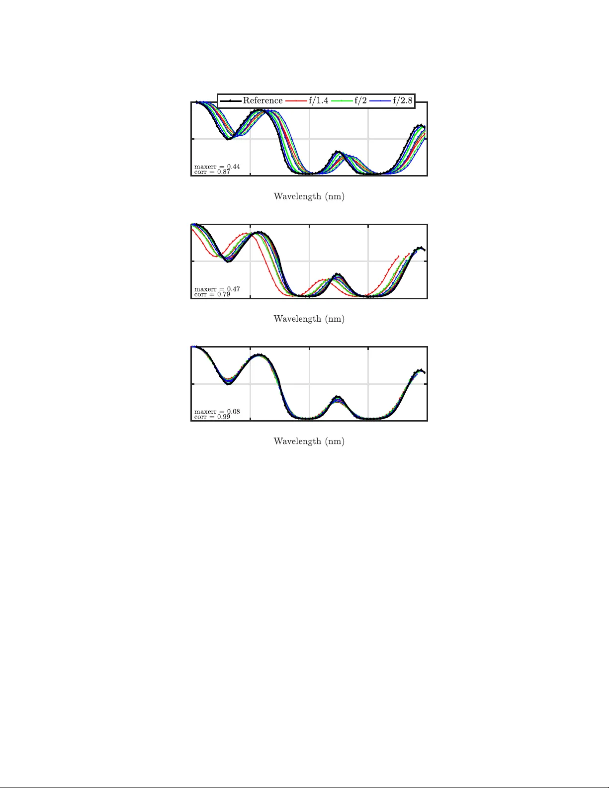
V i g n e t t e d - a p e r t u r e c o r r e c t i o n f or sp ec tr al c a m e r a s wi th in te gr at ed th in -f il m Fab r y- Pé rot f i l t e r s T H O M A S G O O S S E N S 1 , 2 , * , B E R T G E E L E N 2 , A N DY L A M B R E C H T S 2 , C H R I S V A N H O O F 2 , 1 1 Department of Electrical Engineering, KU Leuven, Leuven 3001, Belgium 2 imec vzw, Kapeldr eef 75, 3001 Leuv en, Belgium * contact@thomasgoossens.be https://orcid.org/0000- 0001- 7589- 5038 Abstract: Spectral cameras with integ rated thin-film F abry-Pérot filters ha v e become increas- ingly impor tant in man y applications. These applications often require the detection of spectral f eatures at specific wa v elengths or to quantify small variations in the spectrum. This can be challenging since thin-film filters are sensitive to the angle of incidence of the light. In pr ior w ork w e modeled and cor rected f or the distr ibution of incident angles for an ideal finite aper ture. Man y real lenses ho w e v er e xperience vignetting. Theref ore in this article w e generalize our model to the more common case of a vignetted aperture, which changes the distr ibution of incident angles. W e propose a practical method to estimate the model parameters and cor rect undesired shifts in measured spectra. This is e xperimentally validated for a lens mounted on a visible to near -infrared spectral camera. © 2019 Optical Society of America. https://doi.org/10.1364/A O.58.001789 1. Introduction Spectral imaging is a techniq ue that combines photography and spectroscop y to obtain a spatial image of a scene and f or each point in that scene and also sample the electromagnetic spectr um at many wa v elengths. This spectrum can be used as a ’fingerpr int ’ to identify different materials in the scene. In some applications, small differences in the spectr um hav e to be quantified. Spectral imaging is required if these differences are too small to be detected with RGB color cameras. Other applications require the detection of spectral features at specific wa v elengths [1]. Theref ore, spectral imaging has the potential to increase selectivity in machine lear ning applications. Also, ha ving a spectrum enables phy sical inter pretation of the acquired spectral data (e.g. f or mater ial identification) [2, 3]. In recent years spectral cameras hav e been dev eloped with integrated thin-film F abry-Pérot filters on each pixel of an imag e sensor [4, 5]. T o obtain an imag e, the sensor ar ra y is placed in the image plane of an objective lens which f ocuses light from the scene onto each pixel. Focused light from a finite aperture widens and shifts the transmittance peak of thin-film F abry-Pérot filters because these filters are angle-dependent [6]. This angle-dependent property causes undesired shifts in the measured spectra which limit the accuracy of the spectral imaging technology . Theref ore cor recting these shifts is important f or improving the perf ormance of man y applications including machine lear ning. In pre vious w ork w e proposed a model that w as used to successfully correct the undesired shifts in measured spectra [6]. How ev er , this model is onl y valid f or a lens that sho w s no significant optical vignetting. In this article w e generalize our or iginal model to allo w f or an aperture with optical vignetting. W e also propose a practical algorithm to estimate the model parameters. The results are therefore of g reat practical impor tance since optical vignetting is a common phenomenon. Ev en more so f or very compact and less e xpensiv e lenses. Hence this paper enables the use of suc h lenses and enables spectral imaging f or more price sensitiv e applications. 2. Theory and methods In this section, we discuss ho w a spectral camera can be modeled (Subsection 2.1) and ho w the effect of an ideal finite aper ture was modeled in earlier w ork (Subsection 2.2). W e extend the model to include optical vignetting (Subsection 2.4 and 2.5) and how to correct for it (Subsection 2.6). W e conclude with an algor ithm to estimate the model parameters (Subsection 2.7). 2.1. Spectral imaging model Fig. 1: A schematic representation of ho w an aper ture f ocuses light on the spectral imaging sensor with integrated thin-film optical filters. In the case of vignetting, par t of the exit pupil is cut off. Only the vignetted exit pupil then contr ibutes to focusing the light. The imaging sy stem used in this ar ticle consists of an objectiv e lens with a finite aperture (e xit pupil) which f ocuses the light onto pix els of an imaging sensor with integrated thin-film interference filters (Fig. 1). The output DN (Digital Number) of a pixel with integ rated filters can be modeled as DN = ∫ λ r λ l T ( λ ) · L ( λ ) d λ . (1) Here L ( λ ) is the ir radiance spectrum of the light incident at the pixel and T ( λ ) is the transmittance of the filter measured under or thogonal collimated light conditions. The gain factors are assumed to be equal to 1 and are theref ore omitted [7]. The limits of the integral describe the bandpass rang e of the spectral camera. For a giv en f-number (characterized by half-cone angle θ cone ) and chief ray angle θ CRA , the effect of the aper ture and optical vignetting on the filter with central w a v elength λ cw l is modeled as a con v olution of T ( λ ) with a kernel K θ cone , θ CRA ( λ ) such that DN = ∫ λ r λ l ( K θ cone , θ CRA ∗ T )( λ ) · L ( λ ) d λ, (2) with ∗ being the conv olution operator and the f-number being the ratio of the effectiv e f ocal length to the diameter of the entrance pupil. Belo w in T able 1, the most impor tant symbols are summar ized. T able 1: List of the main symbols and their meaning. Symbol unit Meaning T( λ ) T ransmittance of a filter under orthogonal collimated conditions λ cw l nm central wa v elength of filter f # f-number f # , W w orking f-number x mm distance from pixel to exit pupil plane d mm distance from optical axis θ CRA rad chief ra y angle θ cone rad half-cone angle of the imag e side light cone R mm Radius of the circular e xit pupil P mm Radius of the projected vignetting circle h mm Dis tance of e xit pupil to entrance circle 2.2. Finite aper ture correction In spectral camera designs where interference filters are spatially ar rang ed behind an objectiv e lens, understanding the impact of f ocused light from a finite aperture becomes essential. In this section we discuss the effect of the angle of incidence on thin-film F abry-Pérot filters and the main results of pr ior work on the effect of f ocused light. Thin-film Fabry-Pérot filters are constr ucted b y combining multiple lay ers of a high and a lo w refractiv e index mater ial [8]. The filters appro ximate beha vior of the ideal F abry-Pérot etalon. The transmittance characteristics of inter f erence filters chang e with the angle of incidence of the light. The larg er the angle of incidence, the more the transmittance peak shifts tow ards shorter wa velengths. The angle-dependent behavior of multilay er thin-film filters can be simulated using the transf er -matrix method [8]. Ho w e v er , f or angles up to 40 degrees it was shown that the filter can be modeled as an ideal F abry-Pérot etalon [8, 9]. This idealized etalon has an effectiv e cavity material with an effectiv e refractiv e index n eff which depends on the mater ials used. The shift in central w a v elength of a thin-film F abry-Pérot filter with effectiv e refractive inde x n eff f or an incident angle φ is well approximated b y ∆ ( φ ) which is defined as ∆ ( φ ) = − λ cw l 1 − s 1 − sin 2 φ n 2 eff ! , (3) with λ cw l the central w a v elength of the transmittance peak. W e hav e chang ed the sign con v ention compared to Eq. (3) in [6]. It is natural to consider a negativ e shift because the central wa v elength becomes shor ter . This shift in central wa v elength can also be modeled as a conv olution of the initial transmittance T ( λ ) with a shifted Dirac distribution such that T φ ( λ ) ∼ T ( λ ) ∗ δ ( λ − ∆ ( φ ) ) . (4) T o model the effect of a finite aper ture, f ocused light can be interpreted as a distribution of incident angles c haracterized b y two parameters: the cone angle θ cone (or f-number) and chief ra y angle θ CRA (Fig. 1). The analy sis can be simplified by decomposing the focused beam of light in contributions of equal angles of incidence. In ear lier work w e hav e sho wn that the effect of the aperture can be modeled b y a conv olution of the transmittance of the filter with a kernel K θ cone , θ CRA ( λ ) [6]. The k ernel w as defined as K θ cone , θ CRA ( λ ) ∼ 2 n 2 eff λ cw l · η n eff r − 2 λ λ cw l ! π tan 2 θ cone , (5) as used in Eq. (2) and with η as it will be defined in Eq . (15) . The chang es in the transmittance of the filters cause undesired shifts in the measured spectra. T w o differences to the cor responding Eq. (15) in [6] must be pointed out. Firs t, because of the change in sign conv ention (see Eq. (3) ), there is a sign difference under the square root sign. Second, in this equation, the symbol η is equal to γ as used in Eq. (15) in [6], where it w as used f or the case without vignetting. In this ar ticle, the symbol γ will be reser v ed f or the more general case of vignetting. In pr ior w ork we show ed that the mean value ¯ λ of the k ernel can quantify the shift in central wa velength. The mean value of the kernel w as asymptotically equiv alent to ¯ λ ∼ − λ cw l θ 2 cone 4 n 2 eff + θ 2 CRA 2 n 2 eff ! , f or θ cone , θ CRA → 0 . (6) This formula can be used to cor rect the measured spectra. The wa velength at which the response of each pixel is plotted is updated as λ new cw l = λ cw l + ¯ λ = λ cw l 1 − θ 2 cone 4 n 2 eff − θ 2 CRA 2 n 2 eff ! . (7) In this ar ticle an impor tant e xtension of the abov e analy sis is presented. The model is generalized to include optical vignetting which is a common phenomenon in many real lenses. 2.3. Vignetting Vignetting is the fall-off in intensity that is observed in an imag e that was taken of a unif ormly illuminated scene. There are many types of vignetting that can occur simultaneously . Examples are the cosine-fourth fall-off, optical vignetting, mechanical vignetting, pixel vignetting and pupil aberrations. The ’cosine-fourth ’ fall-off, also called natural vignetting is an effect intrinsic to e v en ideal thin lenses. It is caused b y projected areas of the lens and pixels and the inv erse square law . It implies that, under cer tain assumptions, the intensity of the light will be scaled by a factor cos 4 θ CRA [10]. In wide-angle lenses the effect is more pronounced and is often corrected f or by design [11, 12]. Optical vignetting occurs due to the phy sical length of a lens sys tem or the position of a limiting aper ture somewhere in the optical path [12, 13]. In essence, lens elements can shade other lens elements (F ig. 2). This causes par t of the light beam to be cut off. The amount of optical vignetting depends on the aperture size and is less pronounced f or smaller apertures (high f-numbers). Ob ject Image Lens A Lens B = Ap erture stop Cut off by vignetting Fig. 2: Illustration of optical vignetting. The off-axis point does not receive light from the complete aper ture stop (lens B). This optical vignetting is caused b y the limited diameter of lens A, causing lens B to be par tiall y shaded [12]. In mechanical vignetting part of the scene is e xternally obstructed by for example the lens hood. This can cause the entrance pupil to be par tiall y shaded [13]. In the proposed model there will be no fundamental difference with optical vignetting. Pix el vignetting is an effect in CMOS digital cameras where the photodiode is positioned at the end of a tunnel in the back end of line of the image sensor [14]. Light can onl y reach the photodiode via the tunnel which when illuminated at oblique incidence, casts a shado w on the photodiode. Pix el vignetting beha v es similar to optical vignetting since it also cuts of par t of the light beam. Pupil aber rations descr ibe ho w the aperture is not unif ormly illuminated [15]. Other types of aberrations cause the e xit pupil to mo v e or chang e in size [16, 17]. In the remainder of this article it is assumed that optical and mechanical vignetting are the dominant effects. U nless when specified, we will use the term ’ vignetting’ and ’ vignetted aper ture ’ to imply optical and mechanical vignetting. 2.4. Modeling a vignetted aper ture A vignetted aper ture is an aper ture that is partially cut off as a result of optical or mechanical vignetting. This aper ture will be seen as a differentl y shaped e xit pupil f or each pixel (Fig. 1). In this ar ticle the ’e xit pupil’ is the imag e of the aperture stop (full circle) and the ’vignetted exit pupil’ is the par t of the e xit pupil still focuses light onto the pixel. An insightful approach to understand the shape of a vignetted aper ture is pro vided b y the variable cone model [11]. This model assumes that there is one finite aper ture (e xit pupil) that is encapsulated in a tube with length h and an entrance circle of radius P (Fig. 3). It also assumes that the incident light is collimated. The e xit pupil is the image of the limiting aperture (aper ture stop) some where in the lens sys tem. The second most limiting aperture will be responsible f or most of the vignetting. The image of this second aperture is modeled by the entrance circle of radius P of the tube in Fig. 3. The projection of this entrance circle onto the plane of the e xit pupil is called the projected vignetting circle. Because of its ph y sical dimensions, the tube casts a shado w onto the e xit pupil plane. The part of the e xit pupil that still contr ibutes to focusing the light is then the intersection of the e xit pupil and the projected vignetting circle (red area in Fig. 3). This remaining par t we will call the ’ vignetted e xit pupil’ . The assumption of collimated light simplifies the analy sis. In real lens systems ho w e v er , the light might not be collimated. Y et, e v en in these cases the e xit pupil is still cut off by some circle [12]. The assumption will theref ore only impact the fitted values f or P and h . θ CRA P R h x d | d r | d v Exit pupil Pro jected vignetting circle Vignetted exit pupil Fig. 3: Optical vignetting is modeled with a finite aper ture (exit pupil) encapsulated in a tube illuminated with collimated light. The tube has an opening of radius P at a distance h . The vignetted exit pupil is the ov erlapping area between the exit pupil and the projected vignetting circle. Only the vignetted e xit pupil still f ocuses light. T o calculate the shape of the vignetted e xit pupil, the distances d and d v need to be defined (Fig. 3). The position of a pixel d is characterized by the distance to the optical axis such that d = x tan θ CRA . (8) The position d v of the center of the projected vignetting circle d v = h tan θ CRA . (9) From Eq. (8) and Eq. (9) it f ollo w s that the relativ e size of h and x causes qualitativ e differences. This is discussed in the ne xt section. The variable cone model offers useful intuition about the behavior of optical vignetting. The larg er the radius P relativ e to R , the larg er d v (and hence θ CRA ) needs to become bef ore par t of the e xit pupil is cut off. This intuitiv el y e xplains why for smaller aper tures (small R), there is less optical vignetting. The variable cone model has been used bef ore to model the intensity f all off. Ho w ev er, it has ne v er been used to calculate the distribution of incident angles. Theref ore, in the ne xt section, w e calculate how the shape of the vignetted e xit pupil chang es the distribution of incident angles f or each pixel. W e then calculate how this distribution impacts the transmittance of the integ rated thin-film Fabry-Pérot filters. 2.5. F ocused light from a vignetted aper ture Each filter has a transmittance T ( λ ) when illuminated under or thogonal, collimated conditions. When used with a lens, and because of vignetting, each filter on the sensor ar ra y sees a different distribution of incident angles. The resulting transmittance is defined as ˆ T θ cone , θ CRA ( λ ) . T o anal yze the f ocused light beam from the vignetted aperture, the light beam can be decomposed in contributions of equal angle of incidence φ (Fig. 4). Each contribution can then be treated separatel y using the tilt angle model from Eq. (4). The resulting transmittance is a linear combination of contr ibutions of the f orm of Eq. (4) , each representing a different angle of incidence. The weight of each contribution is the infinitesimal area d A of the aperture that contr ibutes to the same angle of incidence φ (marked by blue in Fig. 4). The transmittance thus becomes ˆ T θ cone , θ CRA ( λ ) = ∬ Vignetted exit pupil T φ ( λ ) d A ∬ Vignetted exit pupil d A , (10) where the normalization is required because of conser v ation of energy . φ Angle of incidence φ Chief ray angle θ CRA 0 Exit pupil Contributions of equal angle of incidence Pro jected vignetting circle Fig. 4: For each θ CRA , the light beam is decomposed in contr ibutions with equal angles of incidence. The weight of a contr ibution is measured by the length of the blue arc within the aperture. Parts of the blue arc can be cut off by the projected vignetting circle. Because of linear ity of the operators, ˆ T θ cone , θ CRA ( λ ) can be wr itten as a conv olution of the transmittance T ( λ ) at orthogonal collimated conditions with a k ernel K θ cone , θ CRA ( λ ) such that ˆ T θ cone , θ CRA ( λ ) = T ( λ ) ∗ ∬ Vignetted exit pupil δ ( λ − ∆ ( φ )) d A ∬ Vignetted exit pupil d A (11) = T ( λ ) ∗ ∬ Vignetted exit pupil δ ( λ − ∆ ( φ )) d A A ( θ cone , θ CRA ) (12) = T ( λ ) ∗ K θ cone , θ CRA ( λ ) . (13) Here A ( θ cone , θ CRA ) is the area of the e xit pupil which, because of vignetting, also chang es with the chief ray angle (see Appendix A). The set of all possible ray s that hav e the same incident angle on a pix el is a hollow cone with half-cone angle φ (the blue cone in Fig. 4). The intersection of this cone with the e xit pupil plane is a circle with radius r = x tan φ . In reality there are only ray s coming from within the e xit pupil. This subset is the par t of the blue circle that lies within the exit pupil (Fig. 4). Its contr ibution is calculated as the infinitesimal area d A of a ring segment (Fig. 5a): d A = 2 γ ( arctan r x ) r d r = 2 γ ( φ ) r d r , (14) with γ ( φ ) being the angle of the arc within the e xit pupil that contributes to the same angle of incidence φ = arctan r x . The angle γ will be defined as a function of tw o other angles: η and ν . The angle η is the angle that describes the contribution in the absence of vignetting (Fig. 5a). It is onl y limited b y the area of the e xit pupil. The effect of vignetting will be that only a subsection of the arc described b y η will be rele vant. This rele v ant par t is calculated using the angle ν . It is the angle that descr ibes what par t of the arc is cut off (Fig. 5a) or k ept (Fig. 5b) by the vignetting circle. T aking into account that r = x tan φ , the angle η ( φ ) is deter mined b y the law of cosines in ∆ XYZ (Fig. 5a) as η ( φ ) = Re  arccos d 2 − R 2 + r 2 2 d r  . (15) By taking the real par t of the in v erse cosine, the case in which there is a complete contr ibuting circle within the aperture is also modeled (Fig. 4) [6]. This is because R e ( arccos z ) = π , f or z ≤ − 1 . Similarl y , ν ( φ ) is defined by applying the law of cosines in ∆ XWV (Fig. 5) such that for h ≥ x , ν ( φ ) = π − Re  arccos d 2 r − P 2 + r 2 2 | d r | r  . (16) By defining d r = d − d v , the abo v e e xpression can be simplified as ν ( φ ) = R e  arccos d 2 r − P 2 + r 2 2 d r r  , (17) which co v ers both h ≥ x and h < x . r R P η r R dA ν d d v | d r | X Y Z V W Exit pupil Pro jected vignetting circle Con tributions of equal angle of incidence Cut off con tribution (a) T op view of the e xit pupil plane f or h ≥ x or equivalentl y d v ≥ d . A part of the contr ibutions of equal angle of incidence is cut off so that only the thick blue line remains. r R P η dA ν d v d | d r | W Y Z V X (b) T op view of the e xit pupil plane f or h < x or equivalentl y d v < d . The part cut off b y the vignetting circle is qualitativ ely different than in Fig. 5a. Fig. 5: Decomposition of the light cone from the aper ture in contr ibutions of equal angle of incidence φ . The w eight of eac h contr ibution is the infinitesimal area d A (blue). Here d is the distance to the pix el from the optical axis. From these definitions and F ig. 5a it follo ws that the resulting contr ibuting arc is defined as γ ( φ ) = ( max ( η ( φ ) − ν ( φ ) , 0 ) h ≥ x min ( η ( φ ) , ν ( φ )) h < x , (18) where ν ( φ ) is the angle that is either cut off or kept, depending on the relativ e size of h and x . In the case h ≥ x , ν represents the angle that is cut off by the vignetting circle (Fig. 5a). Theref ore it must be subtracted from η . The max operator is needed because there is either a positiv e contribution or no contribution. A negativ e angle for γ has no ph y sical meaning. In the case h < x , ν represents the angle of the arc that is not cut off (Fig. 5b). This is modeled b y taking the mininum of η and ν . T o w ork with the angle of incidence φ , r is substituted with r = x tan φ such that d A = 2 x 2 γ ( φ ) tan φ cos 2 φ d φ . (19) The integ ral then becomes K θ cone , θ CRA ( λ ) = ∫ φ max φ min 2 x 2 γ ( φ ) tan φ cos 2 φ δ ( λ − ∆ ( φ )) d φ A ( θ cone , θ CRA ) . (20) Here φ min and φ max are the smallest and larges t incident angles coming from the aperture (See Appendix B). An asymptotic appro ximation of the kernel is K θ cone , θ CRA ( λ ) ∼ 2 n 2 eff λ cw l · γ  n eff r − 2 λ λ cw l  A ( θ cone , θ CRA ) x 2 , (21) as used in Eq. (2). For the derivation see Appendix A. Initially , the kernel in Eq. (21) is equivalent to the kernel in the ideal finite aper ture case (Eq. (5) ). After the onset of vignetting, the kernel is cut-off (Fig. 6). Because the kernel is less wide, the resulting transmittance will be shifted less. In the next section w e der iv e how to calculate this shift. Fig. 6: The shape of the kernel is qualitativ ely sho wn f or different regimes of θ CRA and θ cone . Vignetting causes the kernel to be cut off. The dotted line continues the shape of the k ernel in the absence of vignetting. 2.6. W a velength correction method Each filter has been designed to sense a specific wa v elength. This wa velength is defined as the central wa v elength λ cw l of the transmittance when illuminated in or thogonal collimated conditions. T o plot the spectrum, the response f or each filter is plotted at this central wa v elength λ cw l . As discussed ho we v er, the actual central w a v elength of the filter depends on the angular distribution of the incident light. Thus, to correctly plot a spectr um, the central wa v elength needs to be corrected f or each filter , taking its phy sical position into account. The shift in central w a v elength can be quantified by the mean of the k ernel (when inter preted as a distribution) [6]. The mean is defined as ¯ λ θ cone , θ CRA = ∫ λ max λ min λ K θ cone , θ CRA ( λ ) d λ ∫ λ max λ min K θ cone , θ CRA ( λ ) d λ (normalized) = ∫ λ max λ min λ K θ cone , θ CRA ( λ ) d λ . (22) In Appendix B we explain ho w to numerically appro ximate this integral. T o calculate the ne w central wa v elength of the filter the mean value ¯ λ is added to the original central wa v elength such that λ new cw l = λ cw l + ¯ λ θ cone , θ CRA . (23) The negativ e mean value is added because the shifts are to w ards shor ter wa v elengths. 2.7. Model parameter estimation In this section a practical algor ithm is presented to estimate the model parameters based on the vignetting profile. The vignetting profile can be measured by illuminating the entrance pupil unif ormly with diffuse light from an integrating sphere. The vignetting profile does not only descr ibe optical vignetting. Natural vignetting, pixel vignetting and pupil aber rations might also be present. An algor ithm is theref ore required to isolate the contribution of optical and mechanical vignetting. Optical vignetting is characterized by an abrupt chang e in the vignetting profile [11]. This abrupt chang e is caused by the vignetting circle whic h suddenl y starts cutting off par t of the e xit pupil. This discontinuity can be exploited to isolate optical vignetting from other contributions to the intensity fall-off. The onset of optical vignetting is when the vignetting circle just touches the border of the aper ture. This happens when the the vignetting circle has mov ed a distance equal to the difference in radii such that d v = P − R . (24) Rearranging gives P − d v = P − h tan θ CRA = R = x tan θ cone . (25) For each vignetting profile measured at a different f-number , an equation of the f orm of Eq. (25) can be written do wn. The corresponding chief ray angles are obtained from the vignetting profile at the point where the abr upt chang e starts. The unkno wn model parameters P and h can then be estimated from solving the (possibl y o v erdetermined) linear sys tem         1 − tan ( θ CRA , 1 ) . . . . . . 1 − tan ( θ CRA , n )         P h ! = ©    « R 1 . . . R n ª ® ® ® ¬ . (26) T o deter mine the radius R of the e xit pupil, the w orking f-number f # , W must be used. The w orking f-number is calculated as ( [18]) f # , W ≈  1 + m m P  f # , (27) with m and m P being the linear and pupil magnification respectivel y . The definition of the f-number then implies that R = x tan θ cone = x 2 f # , W . (28) 3. Experimental validation In this section, w e estimate the model parameters and demonstrate that using Eq. (23) the shifted spectra in measurements can be cor rected. 3.1. Experimental setup W e make use of Imec’ s VNIR Snapscan camera [19]. In the Snapscan the image sensor is placed behind the lens and its position can be controlled using an automated translation stag e. This makes the sys tem ideally suited for controlling the chief ray angles. The Snapscan is used with an Edmund Optics 16 mm C Series VIS-NIR fix ed f ocal length lens because it has large chief ray angles and has considerable vignetting. T o efficiently compare different points in the scene, a color filter w as placed in front of the lens. The scene w as filled with a unif orm white ref erence tile (Fig. 7a). The combination of the filter and white reference effectivel y creates a scene-filling uniform spectral tar get. The transmittance of the color filter is calculated using a flat-fielding approach. This requires taking three images: a dark image (no light) and tw o images of the white ref erence tile, one with and one without color filter . Using the notation of the spectral imaging model (Eq. (2) ), the transmittance is then calculated as transmittance = DN filter − DN dark DN white − DN dark . (29) (a) Imec’s Visible Near -Infrared Snapscan cam- era. (b) Integ rating sphere to measure vignetting pro- files. Fig. 7: Experiment al setups. The Edmund Optics 16 mm lens is f ocused at the target sur f ace (approx. 24 mm from the lens). 3.2. Model parameter estimation W e apply the model parameter estimation method from Eq. (26) to an Edmund Optics 16 mm lens. The exit pupil x = 21 mm , linear magnification m = 0 . 06 and pupil magnification m P = 1 . 3 . The filters ha v e an effective refractiv e index of n eff = 1 . 7 . The vignetting fall-off profiles w ere measured using a camera with a panchromatic imag e sensor . The camera was illuminated with unif orm light from an integrating sphere (Fig. 7b). In the vignetting profiles there are sev eral discontinuities, marked by black dots in Fig. 8. T o isolate the discontinuities in the vignetting profile we f ound that they are best visualized when the vignetting profile is divided b y the profile measured f or a high f-number (Fig. 8). Since for this high f-number there is no optical vignetting, this approach seems to cancel out some of the other contr ibutions. This operation is merel y for visualization pur poses and does not impact the fitting procedure since the position of the discontinuities remain unchang ed. From Fig. 8 and Eq. (26) it follo ws that the f ollo wing ov erdeter mined sys tem must be sol v ed:          1 − tan ( 0 . 38 ◦ ) 1 − tan ( 9 ◦ ) 1 − tan ( 13 ◦ ) 1 − tan ( 15 . 4 ◦ )          P h ! = ©     « 7 . 1715 5 . 0201 3 . 5858 2 . 5100 ª ® ® ® ® ¬ . (30) Where each angle corresponds to a blac k dot on Fig. 8. And R i was deter mined using Eq. (28) . The solution of the o v erdeter mined sys tem, using the Moore–Penrose in v erse, is P h ! = 7 . 4236 16 . 991 ! . (31) W e are in the h < x regime because 16 . 99 < 21 mm. The deviations from the model prediction mean that there are other effects that contribute to the vignetting profile. Ne v er theless, the onset of vignetting, as marked b y the black dots, can be predicted very well. The deviations might be due to the f act that natural vignetting chang es with the aper ture size [10] or because of pupil aberrations. How e v er , as w e will see in the results, these deviations hav e little impact on the cor rection of the shifted spectra. 0 5 10 15 0.4 0.5 0.6 0.7 0.8 0.9 1 Fig. 8: Vignetting profile f or Edmund Optics 16 mm lens measured f or different f-numbers. Using the estimated model parameters from Eq. (31) , the vignetting profile is predicted (black line). 3.3. Experiment and data analysis In each e xper iment, transmittance imag es (Eq. (29) ) are taken at different f-numbers using the setup shown in F ig. 7a. For each f-number , the spectr um is plotted at three chosen positions that correspond to chief ray angles of 1 . 9 ◦ , 10 . 3 ◦ and 17 . 4 ◦ . T o plot the spectra, the output (Eq. (29) ) f or each pixel is plotted at the or iginal central wa velength λ cw l of the deposited filter . Because of this, the shifts of the filters tow ards shor ter wa velengths creates the illusion that the spectra mov e tow ards longer wa v elengths. The actual spectrum of the incident light, of course, does not chang e. W e plot three graphs. The first is the uncor rected transmittance f or all the samples. The second is the transmittance cor rected assuming an ideal finite aper ture (Eq. (7) ). The third is the transmittance cor rected using the vignetting model (Eq. (23)). For compar ison, we also simulate the results of the e xperiment. The simulation is done by combining Eq. (2) and Eq. (29). For each plot we also displa y tw o metr ics that quantify the impro v ement: the correlation coefficient and the maximum error . These quantities were calculated for each pair of spectra. Only the w orst values are displa y ed on the graph. 3.4. Results The uncor rected transmittances sho w clear variations compared to the ref erence measured at f / 8 (Fig. 9a). The variations are plotted for each f-number separatel y in (Fig. 10) The different spectra measured at f / 1 . 4 are shifted less compared to the higher f-numbers (Fig. 10). Intuitiv el y one w ould e xpect larger de viations for smaller f-numbers. Without vignetting at f / 1 . 4 , the spread betw een the measured spectra for filters centered at 700 nm should be about 11 nm while the measured spread is about 2 nm. Theref ore, if one ignores the presence of optical vignetting and uses Eq. (7) to correct the central wa v elengths, the shifts are significantly o v ercorrected (Fig. 9b and 10b). Because optical vignetting is more pronounced f or smaller f-numbers, these are o v ercorrected the most. If the vignetting model is used to cor rect the central wa v elengths using Eq. (23) , the different spectra align v ery w ell, as desired (Fig. 9c). In the simulation, v ery similar results are obtained (Fig. 11). This sho ws that the model can also be used to predict the impact of a lens with optical vignetting on the measurements. It also sho w s that ev en in simulation some variation remains after correction (Fig. 11c). This is because the kernel does not onl y shift the filters but also chang es their shape (Fig. 6). The differences between Fig. 9b and Fig. 9c can be better understood by compar ing E q . (6) and E q . (22) visuall y (Fig. 12). This figure summar izes the effect of vignetting on the shift of the filters. It show s that after the onset of vignetting, Eq. (6) starts to o v erestimate the shift. The near constant v alue of the red cur v e also explains wh y the spread in shift f or f / 1 . 4 is only about 2 nm. 650 700 750 800 850 0 0.5 1 (a) Measured transmittance (uncorrected) 650 700 750 800 850 0 0.5 1 (b) Cor rected using Eq. (7) 650 700 750 800 850 0 0.5 1 (c) Cor rected using vignetting model Eq. (23) Fig. 9: Edmund Optics 16 mm lens . The uncor rected reflectance values demonstrate position and f-number dependent shifts. The spectr um is plotted at three chosen positions that correspond to chief ra y angles of 1 . 9 ◦ , 10 . 3 ◦ and 17 . 4 ◦ . Without consider ing vignetting, the model o v ercorrects the shifts (Fig. 9b). Using Eq. (23) with the estimated model parameters, the correction is significantly improv ed. 700 750 0 0.5 1 700 750 0 0.5 1 700 750 0 0.5 1 (a) Measured transmittance (uncorrected) 700 750 0 0.5 1 700 750 0 0.5 1 700 750 0 0.5 1 (b) Cor rected using Eq. (7) Fig. 10: Close-up of a region in Fig. 9 for each separate f-number . The spread of the spectra for f / 1 . 4 is smaller than f or larg er f-numbers. The cor rection with Eq. (23) is not shown here. 650 700 750 800 850 0 0.5 1 (a) Measured transmittance (uncorrected) 650 700 750 800 850 0 0.5 1 (b) Cor rected using Eq. (7) 650 700 750 800 850 0 0.5 1 (c) Cor rected using vignetting model Eq. (23) Fig. 11: Simulated Edmund Optics 16 mm lens . This is a simulation of the e xper imental conditions of Fig. 9. The shifts in the uncor rected and cor rected spectra (Eq. (23) ) are near ly identical to the real measurements. 0 5 10 15 -20 -15 -10 -5 Fig. 12: N umer ical approximation of the mean v alue compared to the asymptotic appro ximation Eq. (6) . The asymptotic appro ximation remains valid until the onset of optical vignetting. Simulated for λ cw l = 700 nm at f-numbers f / 1 . 4 (red), f / 2 (green) and f / 2 . 8 (blue). 4. Discussion The results demonstrate that the proposed method can be used to cor rect undesired shifts in measurements in the presence of optical or mechanical vignetting. Correcting these position-dependent shifts is impor tant f or improving the per f or mance of machine learning applications. And because vignetting is a common phenomenon, our method will be rele vant for many practical applications. The method is po w erful since it can treat a lens as a black -box. This is impor tant since often a complete phy sical model of the lens is una vailable. But e v en when a full model is a v ailable, it is still unpractical to get an idea of the dominant effects and ho w to cor rect for them. Our method offers a v ery practical wa y to isolate the effect of optical vignetting and estimate the model parameters to predict and cor rect it. T o mak e the effect of optical vignetting more understandable, more analytical studies on the subject are needed. Cur rentl y , the mean of the kernel is calculated numer icall y . An anal ytical appro ximation of the mean in the vignetting regime w ould be useful f or intuitiv e understanding and quick calculations. The vignetting model presented in this paper successfully generalizes the model from pr ior w ork [6]. Ho w e v er , the model also has some potential limitations which are discussed belo w . Firs t, there is the assumption that the vignetting circle mov es propor tional to tan θ CRA (Eq. (9) ). This might not be a good approximation for some lenses. The equation how e v er can be easily substituted without ma jor changes to the cor rection method. Second, pupil aberrations might cause changes in the radii of the exit pupil and projected vignetting circle. Pupil aber rations will be the topic of future w ork. Third, theoretically there can multiple projected vignetting circles simultaneously present in the system. This means that the aperture is cut off in more complex w ay s. One e xample is pix el vignetting, which also limits the cone of light that can reach the photodiode. This effect was not studied in this ar ticle. How e v er , in Fig. 8, f or f/1.4, there is arguabl y a second discontinuity around θ CRA ≈ 11 ◦ . The e xtension to multiple vignetting circles could be in v estig ated fur ther . Ho w e v er , in our e xperiments the additional g ains would be negligible. 5. Conclusion In many applications it is impor tant that the measured spectra are independent of the lens and the position of the targ et in the scene. Shifts in the measured spectra are caused b y the sensitivity of the filters to the angle of incidence and must be corrected f or . In previous w ork we demonstrated this for real lenses that e xhibited no vignetting. Vignetting, ho w e v er , is a common phenomenon in real lenses and must be tak en into account f or accurate cor rection. Thus, in this ar ticle w e generalized our model for a vignetted aper ture. W e demonstrated that this generalization is vital f or cor recting the observed shifts in measured spectra. Because vignetting is so common, our method has the potential to impro v e the per f or mance of man y spectral imaging applications. These will mostl y be applications that use fast lenses (large aperture) or low cost lenses but still require high spectral accuracy . Appendix A. Closed-form solution of the kernel In this section w e der iv e a closed-f orm solution of the kernel and derive the anal ytical approxi- mation given in Eq. (21). The der iv ation of the closed-form solution is identical to der iv ation presented in prior w ork (see [6]) up to a fe w minor modifications. First, the shape of the e xit pupil chang es and theref ore also the distr ibution of incident angles. Thus γ is defined by Eq. (18) instead of γ ( φ ) = η ( φ ) . Second, the area of the vignetted e xit pupil chang es. Theref ore the kernel should be nor malized accordingly . Theref ore K θ cone , θ CRA ( λ ) = ∫ φ max φ min 2 x 2 γ ( φ ) tan φ cos 2 φ δ ( λ − ∆ ( φ )) d φ ∬ Vignetted exit pupil d A , = ∫ φ max φ min 2 x 2 γ ( φ ) tan φ cos 2 φ δ ( λ − ∆ ( φ )) d φ A ( θ cone , θ CRA ) , (32) with ∆ ( φ ) defined in Eq. (3) and A ( θ cone , θ CRA ) being the area of the vignetted e xit pupil which is defined as [11] A ( θ cone , θ CRA ) = P 2 ( α − sin ( α ) cos ( α )) + R 2 ( β − sin ( β ) cos ( β )) , (33) with α = Re  arccos P 2 − R 2 + d 2 v 2 P d v  (34) β = Re  arccos R 2 − P 2 + d 2 v 2 R d v  , (35) and d v = h tan θ CRA and R = x tan θ cone . The integral in Eq. (32) can be re written using the Hea viside function H (· ) . If we define Π ( φ ) = H ( φ − φ min ) − H ( φ − φ max ) , then K θ cone , θ CRA ( λ ) = ∫ ∞ −∞ 2 x 2 γ ( φ ) tan φ cos 2 φ δ ( λ − ∆ ( φ )) Π ( φ ) d φ A ( θ cone , θ CRA ) . (36) T o proceed w e use the same steps as described in Appendix A of [6], the only difference being the difference in sign con v ention f or shift. The closed-f or m analytical solution to Eq. (36) can be f ormulated as K θ cone , θ CRA ( λ ) = g ( λ ) γ ( ∆ − 1 ( λ )) A ( θ cone , θ CRA ) x 2 Π  ∆ − 1 ( λ )  , (37) with γ as defined in Eq. (18) and the function g ( λ ) containing all remaining terms: g ( λ ) = 2 n 2 eff λ cw l ·  1 + λ λ cw l  1 + 2 n 2 eff λ λ cw l + n 2 eff λ 2 λ 2 cw l ! 2 (38) = 2 n 2 eff λ cw l + O  λ λ cw l  , f or λ λ cw l → 0 . (39) The notation O (·) is the Big O notation which descr ibes the limiting behavior of the er ror ter m of the approximation. Combining the appro ximation in Eq. (38) with ∆ − 1 ( λ ) = arcsin n eff s − λ λ cw l  2 + λ λ cw l  ! = n eff r − 2 λ λ cw l + O λ 3 / 2 λ 3 / 2 cw l ! , f or λ λ cw l → 0 , (40) the kernel can be appro ximated as K θ cone , θ CRA ( λ ) ∼ 2 n 2 eff λ cw l · γ n eff r − 2 λ λ cw l ! A ( θ cone , θ CRA ) x 2 . (41) The only difference with the result from earlier w ork (Eq. (21) ) is the value of γ and that the area of the vignetted exit pupil no w also varies with θ CRA . B. Calculating the mean of the kernel The mean ¯ λ is required in the central wa v elength cor rection f ormula of Eq. (23) . The mean is defined by the integ ral ∫ λ max λ min λ K θ cone , θ CRA ( λ ) d λ . (42) In this ar ticle we numer icall y appro ximated the mean value and used this value for cor rection. For this, the limits λ min and λ max of the integral need to be known. By constr uction γ ( φ ) becomes zero where needed (Eq. (18) ). Because of this and the f act the shift is alwa y s less than or equal to zero, the upper limit can alwa y s be taken zero in numer ical integration. Theref ore λ max = 0 . The low er integration limit ho w e v er should be kno wn ex actly since there is no theoretical limit to its neg ativ e value. For each case, there are tw o options. The maximal radius is constrained by either the exit pupil or the projected vignetting circle. If it is constrained by the exit pupil, r max = R + d . If it is constrained b y the vignetting circle, the result depends on whether h ≥ x or h < x . In the case that h > x , the kernel becomes zero if η = ν . The maximal radius if f ound by equating Eq. (15) and Eq. (17) and solv e to r such that r = ± p ( d − d r )[ d ( P 2 − d 2 r ) + d r ( d 2 − R 2 )] d − d r , (43) of which only the positive solution is meaningful. For h < x , the maximal radius is r = P + d r . The maximal radius r max f or all cases can be f ormulated compactly as r max =        min ( R + d , P + d r ) h < x min  R + d , √ ( d − d r )[ d ( P 2 − d 2 r ) + d r ( d 2 − R 2 )] d − d r  h ≥ x . (44) The min function models that either the exit pupil or the projected vignetting circle is the limiting circle. From r max , the maximal incident angle φ max can be calculated. By definition, φ max = arctan r max x . And finally , using Eq. (3), λ min = ∆ ( φ max ) . (45) Using the chosen integration limits, the solution is then appro ximated using a left Riemann sum. A step size = 0.01 nm was used. Ho w e v er f or small values of θ cone , the kernel will conv erge to a Dirac distribution. Theref ore a much smaller step size might be required. Instead it is advised to use the asymptotic appro ximation Eq. (6) . In the presence of optical vignetting the asymptotic approximation is valid f or d v < P − R . Or alter nativ el y , θ CRA < arctan P − R h . (46) This condition specifies the onset of vignetting, after which the numer ical solution should be used. The numerical solution and the asymptotic appro ximation are both plotted in F ig. 12. This method is implemented in Code 1. A usage ex ample is giv en in Code 2. Ackno wledgements W e thank Nick Spooren f or proofreading the manuscript. References 1. P . Shipper t, “Why Use Hyperspectral Imagery?” Earth Sci. 70 , 377–379 (2004). 2. G. Lu and B. Fei, “Medical h yperspectral imaging: a revie w .” J. biomedical optics 19 , 10901 (2014). 3. A. Go wen, C. O’Donnell, P . Cullen, G. Downe y , and J. Fr ias, “Hyperspectral imaging – an emerging process analytical tool f or food quality and safety control, ” Trends Food Sci. & T echnol. 18 , 590–598 (2007). 4. B. Geelen, N. T ack, and A. Lambrechts, “A compact snapshot multispectral imager with a monolithically integrated per -pix el filter mosaic,” Proc. SPIE 8974 , 89740L (2014). 5. N. T ack, A. Lambrechts, P . Soussan, and L. Haspeslagh, “A compact, high-speed, and lo w-cos t hyperspectral imager, ” Proc. SPIE 8266, Silicon Photonics VII 32 , 82660Q (2012). 6. T . Goossens, B. Geelen, J. Pichette, A. Lambrechts, and C. V an Hoof, “Finite aper ture correction f or spectral cameras with integ rated thin-film F abry-Perot filters, ” Appl. Opt. 57 , 7539–7549 (2018). 7. J. R. Janesick, Photon transfer (SPIE press San Jose, 2007). 8. H. A. Macleod, Thin-film optical filters (CR C press, 2001). 9. C. R. Pidgeon and S. D. Smith, “Resol ving Po wer of Multilay er Filters in Nonparallel Light, ” J. Opt. Soc. Am. 54 , 1459 (1964). 10. I. C. Gardner, “V alidity of the cosine-fourth-pow er law of illumination, ” J. Natl. Bureau Standards 39 , 213–219 (1947). 11. N. Asada, A. Amano, and M. Baba, “Photometr ic calibration of zoom lens sys tems, ” Proc. - Int. Conf. on Pattern Recognit. 1 , 186–190 (1996). 12. W . J. Smith, Moder n Optical Engineering (2000). 13. S. F. Ray , Applied Photogr aphic Optics: Lenses and Optical Systems for Photog raphy , Film, Video, Electronic and Digital Imaging (Focal, 2002). 14. P . B. Catrysse and B. a. W andell, “Optical efficiency of image sensor pixels.” J. Opt. Soc. Am. A, Opt. image science, vision 19 , 1610–1620 (2002). 15. M. Aggarwal, H. Hua, and N. Ahuja, “On cosine-fourth and vignetting effects in real lenses, ” Int. Conf. on Comput. Vis. 1 , 472–479 (2001). 16. L. Hazra, “Introduction to Aberrations in Optical Imaging Systems by José Sasián, ” J. Opt. 42 , 293–294 (2013). 17. J. Sasian, “Interpretation of pupil aberrations in imaging sys tems, ” Proc. SPIE 6342 , 6342 – 6342 – 4 (2006). 18. R. Kingslake, Optics in Photogr aphy , vol. 6 (SPIE Press Monog raph, 1992). 19. J. Pichette, W . Charle, and A. Lambrechts, “Fas t and compact inter nal scanning CMOS-based hyperspectral camera: the Snapscan,” Proc. SPIE 10110 , 1011014 (2017).