Semantic Segmentation of Seismic Images

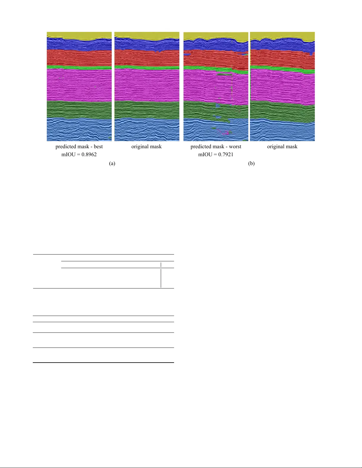
Semantic Segmentation of Seismic Images Daniel Civitar ese 1 ∗ , Daniela Szwarcman 1 , 2 , Emilio V ital Brazil 1 and Bianca Zadrozny 1 1 IBM Research 2 PUC-Rio { sallesd, daniszw , e vital, biancaz } @br .ibm.com Abstract Almost all work to understand Earth’ s subsurface on a large scale relies on the interpretation of seismic surveys by experts who se gment the sur- ve y (usually a cube) into layers; a process that is very time demanding. In this paper , we present a ne w deep neural network architecture specially designed to semantically se gment seismic images with a minimal amount of training data. T o achie ve this, we make use of a transposed residual unit that replaces the traditional dilated con v olution for the decode block. Also, instead of using a prede- fined shape for up-scaling, our network learns all the steps to upscale the features from the encoder . W e train our neural netw ork using the Penobscot 3D dataset; a real seismic dataset acquired of fshore Nov a Scotia, Canada. W e compare our approach with two well-kno wn deep neural network topolo- gies: Fully Conv olutional Network and U-Net. In our e xperiments, we sho w that our approach can achiev e more than 99% of the mean intersection ov er union (mIOU) metric, outperforming the ex- isting topologies. Moreover , our qualitative results show that the obtained model can produce masks very close to human interpretation with very little discontinuity . 1 Introduction Seismic surveys are the most used data to understand the sub- surface nowadays, which is an indirect measure that has a long and complex chain of computational processing. In one of the crucial steps in seismic interpretation, the ex- pert must find the separation between two bodies of rock hav- ing dif ferent physical properties; this separation (the contact between tw o strata) can be called horizons. T o be able to mark the horizons the geoscientist analyzes slices (images) of the seismic cube (survey) looking for visual patterns that could indicate the strata [ Randen et al. , 2000 ] . This task is time-consuming and it o verloads human interpreters as the amount of geophysical information is continually increasing. T ypically the expert must analyze more than 20% of all lines ∗ Contact Author of the seismic cube, which can mean thousands of images in some recent surve ys. Both industry and academia hav e been adv ancing the per- formance of automated and semi-automated algorithms to e x- tract features from seismic images [ Randen et al. , 2000 ] . In the past, most of the previous attempts to automate parts of the seismic facies analysis process relied mainly on tradi- tional computer vision (CV) techniques. For instance, [ Gao, 2011 ] studied the application of gray level co-occurrence ma- trix (GLCM) methods; some more recent work introduced other imaging processing techniques like phase congruency [ Shafiq et al. , 2017 ] , the gradient of te xture (GoT) [ W ang et al. , 2016 ] , local binary patterns (LBP) [ Mattos et al. , 2017 ] or ev en combining more than one method [ Ferreira et al. , 2016 ] . In the last tw o years, the interest in applying machine learn- ing techniques to process seismic data has increased, and last year there was ev en a workshop at NeurIPS called Machine Learning for Geophysical & Geochemical Signals . [ Chevitarese et al. , 2018d ] present a study about seis- mic facies classification using con volutional neural networks. They test the models on two real-w orld seismic datasets [ Ba- roni et al. , 2018a; Baroni et al. , 2018b ] with promising re- sults. In [ Chevitarese et al. , 2018b ] , the authors show ho w transfer learning may be used to accelerate and impro ve train- ing on seismic images, and in [ Chevitarese et al. , 2018a ] they applied the transfer technique to semantically segment rock layers. Howe v er , all these articles lack a detailed discussion about the effect of different network topologies, training proce- dures, and parameter choices, being focused on the domain application rather than on the machine learning aspects. T o address this lack of detail, [ Chevitarese et al. , 2018c ] present deep learning models specifically for the task of classification of seismic facies along with a detailed discussion on how dif- ferent parameters may af fect the model’ s performance. In this work, the y present four different topologies: Danet1, Danet2, Danet3, and Danet4, that are able to reach 90% of classifica- tion accuracy with less than 1% of the a v ailable data. 1.1 Semantic segmentation of seismic images Seismic facies segmentation consists of generating dense pixel-wise predictions that delineates the horizons in seismic images. T o the best of our knowledge, [ Chevitarese et al. , 2018a ] presented the first study on applying deep learning models to seismic facies segmentation. The authors in [ Alau- dah et al. , 2019 ] presented a similar work using the same dataset based on decon volutional neural networks, but show- ing not so good results in the final segmentation. Additionally to the stratigraphic interpretation of an entire seismic cube, other works have demonstrated how CNN can successfully segment fragments of seismic data. In [ W alde- land et al. , 2018; Shi et al. , 2018; Zeng et al. , 2018 ] , a CNN is used to identify an entire salt structure where the output image is very close to the ground truth. The authors in [ Zeng et al. , 2018; Karchevskiy et al. , 2018 ] uses a segmentation process to delineate salt domes in a giv en seismic. [ Chevitarese et al. , 2018a ] introduces a deep neural net- work topology for segmentation showing good results on seismic data based on existing work on fully conv olutional networks [ Long et al. , 2015 ] . Howe ver , they do not discuss the topology nor the training parameters. Furthermore, there is no performance comparison with network topologies in the literature used for semantic segmentation. Here, we develop deep neural models specifically for the semantic segmentation task using state-of-the-art concepts and tools to train and predict seismic facies efficiently . Our goal is to reduce the amount of labeled data the geoscien- tist has to produce to have all the slices in one cube correctly segmented. In other words, with a minimum number of anno- tated images, we want to produce efficient and good quality segmentation in the rest of the cube. W e explore the network topology to reduce the number of parameters and operations but yet improve the performance of test data. Additionally , we analyze the performance im- pact of dif ferent input sizes and number of training e xamples. Finally , we compare our results to those obtained by using well-known topologies applied to the seismic facies segmen- tation task in the literature. W e divide this paper into fiv e sections. In the following section, we present the dataset and the pre-processing proce- dure. Next, in the Network Architectures section, we present the techniques used to design our models and discuss the net- work topologies. In the Experiments section, we describe training parameters and the experimental results. Finally , we present the conclusions and future work in the last section. 2 Dataset In this section, we describe the dataset used in our experi- ments and the data preparation process. 2.1 Penobscot Seismic Dataset The generation of seismic images is a sophisticated process which comprises many steps. The first one is data acqui- sition, which requires an intense sound source, such as an air gun, to direct sound wav es into the ground. These waves pass through different layers of rock (strata) and are reflected, returning to the surface, where geophones or hydrophones record them. This signal is then processed in an iterati ve pro- cedure to generate the seismic images. Finally , interpreters analyze the resulting images and discriminate the different categories – or facies [ Mattos et al. , 2017 ] . These categories represent the ov erall seismic characteristics of a rock unit that reflect its origin, differentiating this unit from the other ones around it [ Mattos et al. , 2017 ] . Penobscot 3D Surv ey [ Baroni et al. , 2018b ] is the publicly av ailable dataset used in this work. It consists of a horizon- tal stack of 2D seismic images ( slices ), creating a 3D vol- ume as depicted in Figure 1. The v ertical axis of this vol- ume represents depth. The remaining axes define the inline and cr ossline directions – red arrows in Figure 1. The inline slices are the images in the cube perpendicular to the inline direction, indicated by the blue blocks in Figure 1. The same idea applies to the crossline slices, which are images along the depth axis and perpendicular to the crossline axis. The Penob- scot dataset contains 481 crossline and 601 inline slices, with dimensions 601 × 1501 and 481 × 1501 pixels, respectiv ely . It is important to mention that we used only inline slices in this work and we removed corrupted or poor-quality images, as indicated by an expert. After removing these images, we ended up with 459 inline slices. depth inline crossline train validation Figure 1: 3D seismic volume with the di vision highlighted in blocks of inline slices. The red arrows indicate inline, crossline and depth directions. In each block, the first slices go to the training set and the rest to the validation set. Geoscientists interpreted and annotated the slices generat- ing a label mask for each one. The experts interpreted sev en horizons: H1, H2, H3, H4, H5, H6, and H7, numbered from the lowest depth to the highest. They di vide the seismic cube into eight interv als with different pattern configurations. Fig- ure 2 b shows the 7 interpreted horizons, creating 8 classes. The geoscientists based their interpretation on configuration patterns that indicate geological factors like lithology , strati- fication, depositional systems, etc. [ Brown Jr , 1980 ] . In the following list we explain briefly the seismic facies of each of the horizon intervals based on the amplitude and continuity of reflectors. 0. ocean. 1. the facies unit is composed of high-amplitude reflectors. Although most of the reflectors are continuous, some hav e diving angles and others are truncated, evidencing a high energy en vironment. 2. the package consists mostly of parallel, high-amplitude reflectors. 3. reflectors are predominantly subparallel and present varying amplitude. 4. reflectors between these horizons are continuous but hav e low amplitude, which makes it difficult to identify them. 5. facies unit containing parallel to subparallel reflectors, like the pre vious interv al, but less continuous. 6. the facies unit is characterized by parallel to subparallel, continuous, high-amplitude reflectors. 7. the facies unit below the 7 th horizon is characterized pri- marily by parallel, concordant, high-amplitude reflec- tors. 0 1 2 5 6 4 3 7 tile label tile label (80 x 120) (128 x 128) (a) (b) (c) Figure 2: (a) Example of an inline slice (we cropped the bottom of the image). (b) The corresponding mask for the input image, showing the eight categories. (c) T ile examples with their respectiv e label masks. For better visualization, the tiles are not on the same scale as (a) and (b). 2.2 Dataset preparation As discussed in [ Mattos et al. , 2017; Chopra and Alex eev , 2006 ] , here we assume that one may identify different cate- gories by their textural features. Therefore, a model that can distinguish textures in an image can be used to separate seis- mic facies. In our segmentation task, we chose to break the seismic im- ages into smaller tiles (Figure 2 (c)), as the original ones are large and would require a more complex model to deal with such a big input size. Also, the original images have a float range around [-30.000, 33.000] and we decided to rescale them to the grayscale range of [0, 255]. Our dataset preparation comprises the following steps: 1. remove corrupted images (indicated by a domain ex- pert); 2. split image files into training, validation and test sets; 3. process images removing outliers, and rescale v alues be- tween 0-255; 4. break processed images into tiles using a sliding windo w mechanism that allows o verlap; As we want to simplify the interpreter job, we must create training, validation and test sets that correspond to the nature of this task, i.e., we should use only data from a single seis- mic cube. W e acknowledge that adjacent slices can be similar since they represent seismic characteristics of neighboring re- gions. F or the same reason, we also expect slices located far from each other in the volume to be less correlated. Howe ver , different cubes represent dif ferent regions that usually do not hav e interchangeable classes or characteristics. Then, for our application, we could not use data from other cubes to test ov erfitting. Keeping that in mind, we used the following scheme to split the cube into training, validation and test sets (see Fig- ure 1): 1. divide the cube into n blocks; 2. in each block, select the first 70% slices for the training set and the remaining 30% for the validation set; 3. (optionally) limit the total number of training slices to be x and randomly select x / n slices in each block so we can simulate limited data scenarios; Follo wing the work in [ Baroni et al. , 2018b ] we merged classes 2 and 3, as class 3 represents a very thin layer (about 20 pixels of depth). Therefore, the final number of classes is sev en. 3 Network architectur es In this paper , we present two new topologies b uilt explicitly for the semantic segmentation of seismic data, Danet-FCN2 and Danet-FCN3. As mentioned before, this kind of image can be very different from common texture images, such as the images in the DTD dataset mentioned in the introduction, where tiles representing textures are larger and have colors that make classes more separable. The proposed architectures use residual blocks [ He et al. , 2016 ] to extract features (encoder), and a novel transposed unit of the same structure to reconstruct the original image with its respectiv e labels (decoder). Contrarily to the previ- ously dev eloped Danet-FCN [ Chevitarese et al. , 2018a ] , these newer models do not have additional fused connections be- tween the encoder and the decoder . In [ Long et al. , 2015 ] , the authors incorporated skip connections in the topology to com- bine coarse, high layer information with detailed, low layer information. On the other hand, He and his colleagues show that shortcut connections and identity after-addition acti v a- tion make information propagation smooth [ He et al. , 2016 ] . In this sense, we merge FCN and ResNet ideas by remo v- ing the shortcuts as in FCN, and U-Net, and by replacing the contracting path with residual units. For the expansiv e part, howe v er , we had to create the in verse operation that we called transposed residual since it was inexistent. In addition to a gain in performance, our new architecture, composed of residual blocks, already implements shortcut paths along with the skip connection, what mak es fuse (FCN and U-Net) oper- ations unnecessary . In Figure 3 we compare all three Danet-FCN topologies, where c stands for a con volution layer , s is the stride, and ru stands for a residual unit. So, an entry c 5 s 2 64 stands for a con volution with 64 filters of size 5 × 5 and stride 2 . The residual configuration we use in this work is the same one Danet FCN2 rest 128 rest 64 c5 s2 32 ct5 s2 32 score res 64 res 128 Danet FCN3 rest 512 c5 s2 64 rest 256 rest 128 ct5 s2 64 score res 128 res 256 res 512 Danet FCN c5 s2 64 convt 256 convt 128 fuse 3 fuse 2 ct5 s2 64 score conv 128 conv 256 rut3 s1 #ch rut3 s1 #ch rut3 s2 #ch rest #ch ct3 s1 #ch ct3 s1 #ch ct3 s2 #ch convt #ch c3 s2 #ch c3 s1 #ch c3 s1 #ch conv #ch res #ch ru3 s2 #ch ru3 s1 #ch ru3 s1 #ch Figure 3: These are the topologies of the three models. On the right, we present the description of each block, where #ch is the number of channels (filters) used in all operations inside it. presented in [ Chevitarese et al. , 2018c ] , described by Equa- tion 1: x ← h ( x ) + F ( x , θ ) y ← f ( x ) (1) where h ( x ) is an identity mapping, and f ( x ) is a ReLU [ Krizhevsk y et al. , 2012 ] function. 3.1 Danet-FCN [ Chevitarese et al. , 2018a ] introduced this model that is based on the VGG-FCN topology presented by [ Long et al. , 2015 ] . In [ Long et al. , 2015 ] , the authors con v ert the fully connected layers at the end of the network structure into 1 × 1 con volu- tions, and append a transposed conv olution to up-sample its input features to the input image size. W e decided to re visit this network not only to compare it with the ones proposed here b ut also to e xtend the discussion about it. The main idea behind Danet-FCN is to hav e a simpler network – instead of using VGG-size structures – that leads to faster training times, and less memory usage. In contrast to its relativ e, VGG- FCN, Danet-FCN only performs conv olutions, and strides in its operations replace pooling to reduce data dimensionality . W e believ e that this is one of the reasons that made Danet- FCN perform remarkably well on the datasets in which it was tested. 3.2 Danet-FCN2 In this work, we propose the use of transposed con volutions to create transposed residual units producing a “mirror” struc- ture similar to the one in U-Net [ Ronneberger et al. , 2015 ] . Figure 4 Although this operation can be more expensi ve com- paring to dilated con volutions, we noticed that it can produce smoother results. The fact that the upscale is learned instead of being predefined by the user may be one explanation for that. Another nice feature we obtained with this ne w residual structure is the creation of links between the encode layers and decode ones, similar to the fuse we have in FCN-16 and FCN-8. Those links improve the segmentation results sub- stantially , as discussed in [ Long et al. , 2015 ] . conv + BN conv + BN + F(x) convt + BN convt + BN + F(x) ReLU Figure 4: On the left we hav e the regular residual structure. On the right, we hav e the proposed transposed residual unit. Figure 3 shows the entire structure of Danet-FCN2. It has a very compact topology allowing it to learn from a minimal number of examples – see T able 2. Also, we noticed that this model is the fastest to train in most of the configurations too. Danet-FCN3 Our biggest topology is similar to Danet-FCN2, b ut compris- ing more residual units with more filters. Comparing to U- Net it has more parameters on one hand, but less operations to compute on the other hand. It is expected a deterioration of the results for smaller datasets since Danet-FCN3 has much more parameters compared to its relati ves Danet-FCN and Danet-FCN2. 4 Experiments Follo wing the idea presented in [ Chevitarese et al. , 2018c ] , we want to inv estigate whether the proposed topologies are useful in a limited data context, which is similar to analyze the influence of the number of slices av ailable for training in the models’ performance. Also, there are only a few small datasets publicly av ailable for training in the Oil and Gas in- dustry . It is important to highlight that the process of annotat- ing seismic images is e xpensi ve and time-consuming. Hence, finding the minimum number of labeled images required to train a model successfully , is valuable for the O&G industry . In this section, we describe the experiments we conducted to accomplish our goals. W e generated different tile datasets from the seismic im- ages by varying the number of slices for the training set: 100, 13, 9 and 5 slices. This allows us to simulate the limited dataset scenarios and analyze models’ performance with a decreasing number of e xamples for training. Based on the results presented in [ Chevitarese et al. , 2018a ] , we selected a tile size of 80 × 120 pixels. In addition, we generated tiles of 128 × 128 pixels so we could compare our netw orks with rel- ev ant models in the literature of semantic segmentation, such as U-Net [ Ronneberger et al. , 2015 ] , which e xpects lar ger in- put images. For both tile sizes, we let 50% of o verlap in each direction. This means that the sliding window skips, for ex- ample, 60 pixels horizontally and 40 pixels vertically in the 80 × 120 tile case. T able 1 summarizes all the generated tile datasets and shows the number of training examples in each one. W e compare our models with slightly modified networks from the literature: FCN16, FCN8 [ Long et al. , 2015 ] and U- Net [ Ronneberger et al. , 2015 ] . In their original applications, the models were designed to handle input images larger than our tiles, but considerably smaller than an entire seismic im- age. Therefore, to fairly compare our models with FCN and U-Net, we decided to make minor changes in their architec- ture to accommodate the smaller or non-square tiles. For the FCN networks, we added a crop mechanism to correct shapes of feature maps in the upsampling part. For the selected tile sizes, we cropped at most 1 pixel from the feature maps, which we can consider that will not af fect the results. For the U-Net, we changed the unpadded con volutions to padded con v olutions, keeping intact the rest of the structure. It is important to mention that, from the selected models in the literature, we only trained FCN-8 using both tile sizes. The other ones would require further changes, or cropping a significant number of pixels in order to comply with the input size of 80 × 120 . 4.1 T raining parameters In all experiments, we fixed the mini-batch as 64 , the weight decay coefficient as 5 × 10 − 4 and the maximum number of epochs as 200 . W e also used the RMSProp optimization al- gorithm [ T ieleman and Hinton, 2012 ] with ν = 0 . 9 , ϕ = 0 . 9 and ε = 1 . 0 in all training sessions. The Xavier method [ Glo- rot and Bengio, 2010 ] of initialization was used in all con vo- lutional kernels while the biases were initialized with zeros. The Danet models hav e batch normalization layers and we chose their parameters  = 1 × 10 − 5 and µ = 0 . 997 . W e also used a learning rate (lr) schedule for the Danet models, to take advantage of the batch normalization benefits. Starting with a relativ ely high lr of 0 . 01 , we performed a stepwise decrease: • epoch = 50 , lr = 0 . 001 • epoch = 100 , lr = 5 × 10 − 4 • epoch = 150 , lr = 1 × 10 − 5 For the FCN and U-Net models, we used a constant learn- ing rate of 1 × 10 − 4 , and dropout with ρ = 0 . 5 , as indicated in the original papers. Also, for the FCN models, we used the same scheme of loading the weights of a V GG16 network previously trained with the ImageNet dataset [ Russakovsk y and others, 2015 ] . W e trained the models using T ensorflo w 1.9, 4 or 2 GPUs K80 (depending on the number of examples) in a Power8 node. Also, we adopted the mean intersection ov er union (mIOU) in the validation dataset as the metric to select the best model during training. One should notice that we calcu- lated the mIOU by averaging the IOU ov er all classes, with the same weights, ev en though they are not balanced. 5 Results and discussion T o compare the trained models, we used the 40 images se- lected for the test set, as mentioned before. Our test procedure for all trained models consists of the following steps: 1. For each image, we break it into non-overlapping tiles of the same size the model was trained with; T able 1: Datasets generated for the experiments 80 × 120 Images 100 13 9 5 T iles 15392 2000 1376 768 128 × 128 Images 100 13 9 5 T iles 7792 1008 688 384 2. we predict the tile masks with the trained model; 3. the entire mask for that image is assembled by uniting the predicted mask tiles; 4. once the entire predicted mask is formed, we calculate the IOU for each class in that image and a verage the results to get the mIOU for the image; 5. finally , when we have the mIOU for all 40 images, we av erage the results to get the o verall response on the test set, which we named here mmIOU. The test procedure enables us to compare the models both quantitativ ely (mmIOU) and qualitativ ely (predicted masks). T able 2 summarizes the mmIOU for all the experiments. T able 2: Experiments results. Image size Model Number of slices (mmIOU) 5 9 13 100 80 × 120 DanetFCN 0.9180 0.9592 0.9700 0.9877 DanetFCN2 0.8932 0.9609 0.9616 0.9874 DanetFCN3 0.8385 0.9689 0.9764 0.9900 FCN8 0.5819 0.7196 0.7389 0.9364 128 × 128 DanetFCN 0.8150 0.8366 0.8272 0.9413 DanetFCN2 0.7618 0.8800 0.8513 0.9360 DanetFCN3 0.7989 0.8484 0.8622 0.9485 FCN8 0.4497 0.5790 0.6605 0.9057 FCN16 0.1524 0.4997 0.5950 0.9369 U-Net 0.1397 0.1431 0.1371 0.1880 For the tile size of 80 × 120 pixels, all Danet models pre- sented a mmIOU higher than 80%, even in the very limited dataset of 5 slices. One can notice that the results deteriorate with the decrease in the number of examples, b ut this ef fect is stronger in the FCN8 and FCN16. In the non-limited context (100 slices in the training set), both FCN8 and FCN16 have a performance similar to the Danet models, but Danet-FCN3 beats them for both tile sizes. On the other hand, we were not able to ef fectiv ely train the U-Net model with our datasets, as shown in the last line of T able 2. The training loss did not con ver ge and the results were poor . Further in vestigation is required to understand the reason for that. A first assumption would be that the input size is still too small for this netw ork. The qualitati ve results for Danet-FCN3 can be seen in Fig- ure 5 and Figure 5. In the 100 slices case, the predicted mask is almost identical to the original one and, in the limited data context, the result is still very close to the mask generated by a human expert. T able 3 complements Figures 5 and 5 as it shows the IOU for each class separately . From these v al- ues, we can see that the classes most affected by the reduced (a) (b) predicted mask - best predicted mask - worst original mask original mask mIOU = 0.8962 mIOU = 0.7921 Figure 5: Masks generated by Danet-FCN3 on the test set, for tiles of size 80 x 120. (a) Best results for the 5 slices case. (b) W orst results for the 5 slices case. amount of examples are classes 1, 3 and 5, b ut the other ones still maintain an IOU higher than 80%. The predicted masks along with the high values of mIOU are a strong indication that our topologies are well suited for the semantic segmenta- tion of seismic images ev en with a restricted number of train- ing examples a v ailable. T able 3: IOU per class Danet-FCN3 and tiles 80 × 120 . IOU per class slices case 0 1 2 3 4 5 6 mIOU 5 best 0.888 0.531 0.983 0.887 0.997 0.989 0.998 0.896 worst 0.889 0.350 0.897 0.596 0.968 0.855 0.989 0.792 100 best 0.991 0.991 0.999 0.990 1.000 0.998 1.000 0.995 worst 0.970 0.983 0.994 0.981 0.999 0.995 0.995 0.988 T able 4: Computational resources. Model name DanetFCN DanetFCN2 DanetFCN3 FCN8 FCN16 UNET Millions of parameters 4.46 6.66 39.2 134.31 134.34 31.03 Millions of operations 3213 1880 10572 9032 - - tile = 80 x 120 Millions of operations 5477 3140 17675 14094 14093 24133 tile = 128 x 128 T able 4 compares the models by the number of parameters and operations. Danet-FCN has the lo west number of param- eters and, at the same time, is the best performing model for the 5 slices training case for both tile sizes. Danet-FCN3 and U-Net have parameters in the same order of magnitude, but U-net has significantly more operations. In this case, we were able to take advantage of the deep residual network and get excellent results while keeping the number of operations sim- ilar to what we find in FCN and U-Net. Comparing T able 4 with T able 2 we can conclude that Danet-FCN2 can be seen as the model with the best balance between performance and efficiency . It has the lowest num- ber of operations and almost 5 times less parameters than U- net while presenting mmIOU above 89% for all cases with 80 × 120 tiles. 6 Conclusion In this work, we designed and compared deep neural models specifically for the task of semantic segmentation of seismic images, which hav e different characteristics than standard im- ages. Our proposed networks combine different features from existing architectures and a novel feature which is the use of a transposed conv olution to create transposed residual units producing a ”mirror structure”. T o the best of our knowledge this feature is novel and could be tested as part of neural mod- els for other types of images and ev en for other tasks. Our experiments sho w that our proposed models lead to significantly better results than the semantic segmentation neural models designed for standard images. Furthermore, we ev aluated these models under the realistic condition that there would be very few examples for training (as few as 5 slices) and showed that we can still achiev e high v alues in the intersection o ver union metric and, through visual inspection, see a good reproduction of the original masks. For future work we want to test the proposed topologies on new seismic datasets. Also, it is important to experiment with more seismic layers being considered by the model, and then increasing the number of facies (classes) recognized by the network. Finally , we want to include to the current data (texture only) the geophysical properties (e.g., v elocity). References [ Alaudah et al. , 2019 ] Y . Alaudah, P . Michalowicz, M. Al- farraj, and G. AlRe gib . A machine learning benchmark for facies classification. , 2019. [ Baroni et al. , 2018a ] L. Baroni, R. M. Silva, R. S. Fer- reira, D. Chevitarese, D. Szwarcman, and E. V ital Brazil. Netherlands f3 interpretation dataset, September 2018. [ Baroni et al. , 2018b ] L. Baroni, R. M. Silva, R. S. Ferreira, D. Chevitarese, D. Szwarcman, and E. V ital Brazil. Penob- scot interpretation dataset, July 2018. [ Brown Jr , 1980 ] L. F . Bro wn Jr . Seismic stratigraphic inter- pretation and petroleum exploration. Course Notes AAPG , 1(16):181p, 1980. [ Chevitarese et al. , 2018a ] D. Chevitarese, D. Szwarcman, R. M. D Silv a, and E. V ital Brazil. Seismic facies seg- mentation using deep learning. In American Association of P etr oleum Geologists (AAPG) , 2018. [ Chevitarese et al. , 2018b ] D. Chevitarese, D. Szwarcman, R. M. D Silva, and E. V ital Brazil. Transfer learning ap- plied to seismic images classification. In AAPG , 2018. [ Chevitarese et al. , 2018c ] D. S. Chevitarese, D. Szwarc- man, E. V . Brazil, and B. Zadrozny . Efficient Classification of Seismic T extures. In IJCNN , jul 2018. [ Chevitarese et al. , 2018d ] D. S. Chevitarese, D. Szwarc- man, R. M. Gama e Silva, and E. V ital Brazil. Deep learn- ing applied to seismic f acies classification: a methodology for training. In Eur opean Association of Geoscientists and Engineers (EA GE) , 2018. [ Chopra and Alex eev , 2006 ] S. Chopra and V . Alexee v . Ap- plications of texture attribute analysis to 3d seismic data. The Leading Edge , 25(8):934–940, 2006. [ Ferreira et al. , 2016 ] R. D. S. Ferreira, A. B. Mattos, E. V i- tal Brazil, R. Cerqueira, M. Ferraz, and S. Cersosimo. Multi-scale ev aluation of te xture features for salt dome de- tection. In IEEE ISM , pages 632–635, 2016. [ Gao, 2011 ] Dengliang Gao. Latest dev elopments in seismic texture analysis for subsurface structure, facies, and reser- voir characterization: A revie w . Geophysics , 2011. [ Glorot and Bengio, 2010 ] X. Glorot and Y . Bengio. Under- standing the difficulty of training deep feedforward neural networks. In 13th International Conference on Artificial Intelligence and Statistics , volume 9 of PMLR , pages 249– 256, May 2010. [ He et al. , 2016 ] K. He, X. Zhang, S. Ren, and J. Sun. Deep residual learning for image recognition. In CVPR , pages 770–778, 2016. [ Karchevskiy et al. , 2018 ] M. Karchevskiy , I. Ashrapov , and L. Kozinkin. Automatic salt deposits segmentation: A deep learning approach. , 2018. [ Krizhevsk y et al. , 2012 ] A. Krizhevsky , I. Sutske ver , and G. E. Hinton. Imagenet classification with deep conv olu- tional neural networks. In Advances in Neural Information Pr ocessing Systems 25 , pages 1097–1105. Curran Asso- ciates, Inc., 2012. [ Long et al. , 2015 ] J. Long, E. Shelhamer , and T . Darrell. Fully con volutional networks for semantic segmentation. In CVPR , pages 3431–3440, 2015. [ Mattos et al. , 2017 ] A. B. Mattos, R. S. Ferreira, R. M. Silva, M. Riv a, and E. V ital Brazil. Assessing texture de- scriptors for seismic image retriev al. In 30th SIBGRAPI , pages 292–299, Oct 2017. [ Randen et al. , 2000 ] T . Randen, E. Monsen, C. Signer, A. Abrahamsen, J. O. Hansen, T . Sæter , and J. Schlaf. Three-dimensional te xture attrib utes for seismic data anal- ysis. In SEG T echnical Pr ogr am Expanded Abstracts 2000 , pages 668–671. 2000. [ Ronneberger et al. , 2015 ] O. Ronneberger , P . Fischer, and T . Brox. U-net: Conv olutional networks for biomedical image segmentation. In International Confer ence on Med- ical image computing and computer-assisted intervention , pages 234–241. Springer , 2015. [ Russakovsk y and others, 2015 ] Olga Russako vsky et al. ImageNet Large Scale V isual Recognition Challenge. IJCV , 115(3):211–252, 2015. [ Shafiq et al. , 2017 ] M. A. Shafiq, Y . Alaudah, G. AlRegib, and M. Deriche. Phase congruency for image understand- ing with applications in computational seismic interpreta- tion. In IEEE ICASSP , pages 1587–1591, 2017. [ Shi et al. , 2018 ] Y . Shi, X. W u, and S. Fomel. Automatic salt-body classification using a deep con volutional neural network. In SEG T echnical Pr ogr am Expanded Abstracts 2018 , pages 1971–1975. 2018. [ T ieleman and Hinton, 2012 ] T . T ieleman and G. Hinton. Lecture 6.5—RmsProp. COURSERA: Neural Networks for Machine Learning, 2012. [ W aldeland et al. , 2018 ] A. U W aldeland, A. C. Jensen, L. Gelius, and A. H. S. Solberg. Conv olutional neural net- works for automated seismic interpretation. The Leading Edge , 37(7):529–537, 2018. [ W ang et al. , 2016 ] Z. W ang, Z. Long, and G. AlRegib . T ensor-based subspace learning for tracking salt-dome boundaries constrained by seismic attributes. In IEEE ICASSP , pages 1125–1129, 2016. [ Zeng et al. , 2018 ] Y . Zeng, K. Jiang, and J. Chen. Auto- matic seismic salt interpretation with deep con volutional neural networks. , 2018.