Accurate Tissue Interface Segmentation via Adversarial Pre-Segmentation of Anterior Segment OCT Images

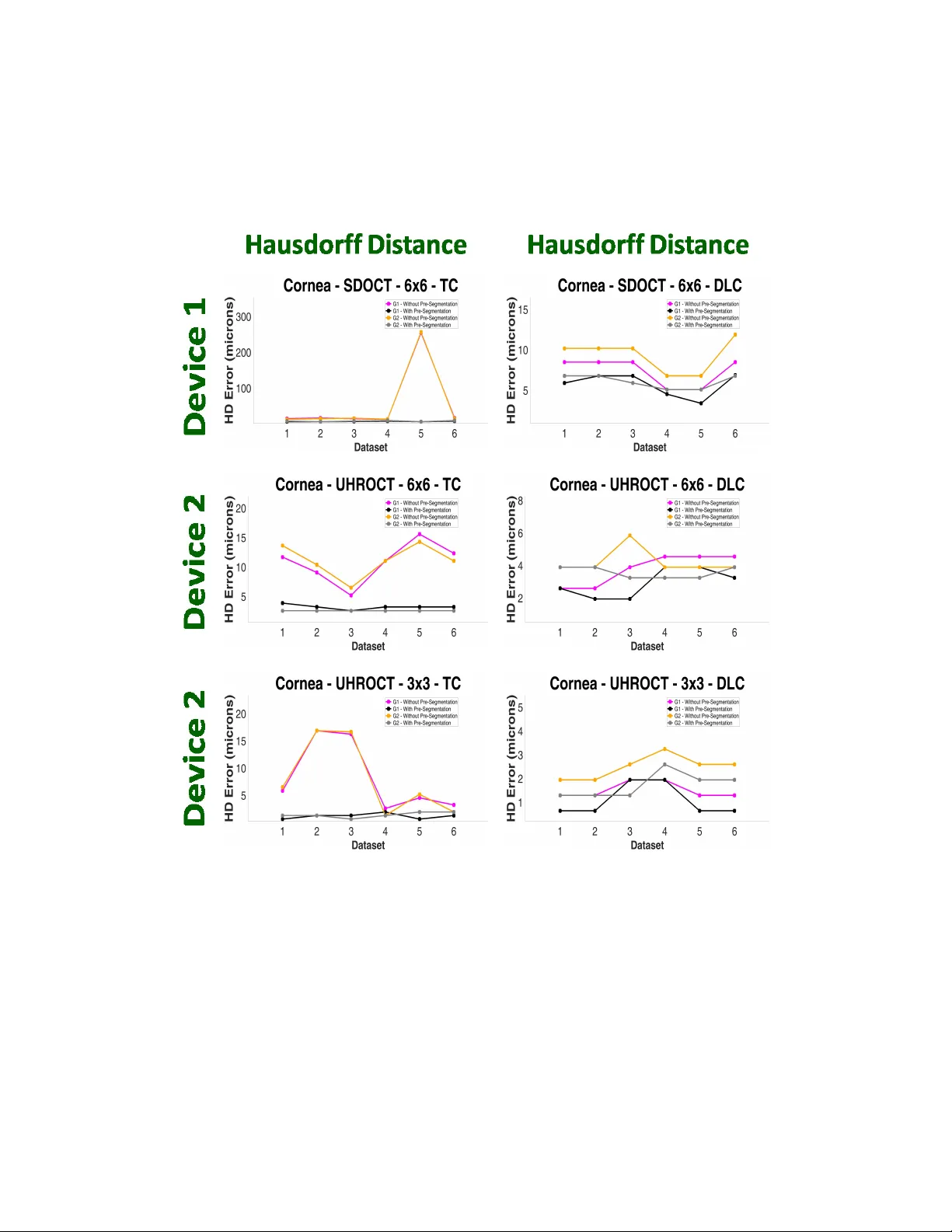
A c c u r a t e T i s s u e I nt er fa ce Se gm en ta ti on vi a A d v e r s a r i a l Pr e- Se gm en ta ti on of An te ri or S e g m e n t OC T I m ag e s J I A H O N G O U Y A N G 1 ∗ , T E J A S S U D H A R S H A N M AT H A I 1 ∗ , K I R A L AT H R O P 2 , 3 , J O H N G A L E O T T I 1 , 2 1 The Robo tics Institute, Carnegie Mellon U niv ersity , USA 2 Department of Bioengineering, Univ er sity of Pittsburgh, USA 3 Department of Ophthalmology, U niv er sity of Pittsburgh, USA ∗ Equal contribution {jiahongo, tmat hai}@andr ew .cmu.edu, lathr opkl@upmc.edu, jgaleo tti@cmu.edu Abstract : Optical Coherence T omography (OCT) is an imaging modality that has been widely adopted f or visualizing corneal, retinal and limbal tissue structure with micron resolution. It can be used to diagnose pathological conditions of the e y e, and f or de veloping pre-operative surgical plans. In contras t to the posterior retina, imaging the anterior tissue s tructures, suc h as the limbus and cornea, results in B-scans that e xhibit increased speckle noise patterns and imaging ar tif acts. These ar tif acts, such as shado wing and specularity , pose a c hallenge dur ing the anal ysis of the acquired volumes as they substantially obfuscate the location of tissue inter f aces. T o deal with the ar tif acts and spec kle noise patterns and accuratel y segment the shallo w est tissue inter f ace, we propose a cascaded neural netw ork frame w ork, which comprises of a conditional Generative A dv ersarial Netw ork (cG AN) and a Tissue Inter f ace Segmentation Netw ork (TISN). The cGAN pre-segments OCT B-scans b y remo ving undesired specular ar tif acts and spec kle noise patterns just abo v e the shallow est tissue interface, and the TISN combines the or iginal OCT image with the pre-segmentation to segment the shallow est interf ace. W e sho w the applicability of the cascaded frame w ork to cor neal datasets, demonstrate that it precisely segments the shallo w est corneal interface, and also sho w its generalization capacity to limbal datasets. W e also propose a h ybr id frame w ork, wherein the cGAN pre-segmentation is passed to a traditional imag e anal ysis-based segmentation algor ithm, and describe the impro ved segmentation per f or mance. T o the best of our know ledge, this is the ﬁrst approach to remo ve sev ere specular ar tif acts and speckle noise patterns (prior to the shallo w est interface) that aﬀects the inter pretation of anterior segment OCT datasets, thereby resulting in the accurate segmentation of the shallo w est tissue interf ace. © 2019 Optical Society of Amer ica under the ter ms of the OS A Open Access Publishing Agreement OCIS codes: (110.4500) Optical coherence tomography; (100.4996) Pattern recognition, neural networks. References and links 1. D. Huang et al., “Optical Coherence T omography”, Science 254 , 1178-1181 (1991). 2. J. Fujimoto et al., “Optical coherence tomography (OCT) in Ophthalmology : Introduction”, Opt. Express 17 (5), 3978-3979 (2009). 3. J. Izatt et al., “Micrometer -Scale R esolution Imaging of the Anterior Eye In Viv o With Optical Coherence T omography”, Arch Ophthalmol. 112 (12), 1584-1589 (1994). 4. K. Lathrop et al., “Optical Coherence T omography as a Rapid, Accurate, Noncontact Method of Visualizing the Palisades of V ogt”, In v est. Ophthalmol. Visual Sci. 53 (3), 1381-1387 (2012). 5. A. Kuo et al., “Cor neal Biometry from V olumetric SDOCT and Compar ison with Existing Clinical Modalities”, Biomed. Opt. Express 3 (6), 1279-1290 (2012). 6. N. V enkateswaran et al., “Optical Coherence T omography for Ocular Surface and Corneal Diseases: A Re view”, Ey e and Vision 5 (1), 1-13 (2018). 7. B. Keller et al., “Real-time Corneal Segmentation and 3D Needle Trac king in Intrasurgical OCT”, Biomed. Opt. Express 9 , 2716-2732 (2018). 8. K. Bizhev a et al., “In Viv o V olumetr ic Imaging of the Human Corneo-Scleral Limbus with Spectral Domain OCT”, Biomed. Opt. Express 2 (7), 1794-1802 (2011). 9. K. Bizhe va et al., “In- Viv o Imaging of the Palisades of V ogt and the Limbal Crypts with Sub-Micrometer Axial Resolution Optical Coherence T omography”, Biomed. Opt. Express 8 (9), 4141-4151 (2017). 10. M. Haagdorens et al., “ A method f or quantifying limbal stem cell niches using OCT imaging”, Br. J. Ophthalmol., 101 (9), 1250-1255 (2017). 11. F . LaRocca et al., “Robus t Automatic Segmentation of Corneal La y er Boundaries in SDOCT Images using Graph Theory and Dynamic Programming”, Biomed. Opt. Express 2 (6), 1524-1538 (2011). 12. L. Ge et al., “ Automatic Segmentation of the Central Epithelium Imaged With Three Optical Coherence T omography Devices ”, Eye & Contact Lens, 38 (3), 150-157 (2012). 13. D. Williams, Y . Zheng, F . Bao, and A. Elsheikh, “ Automatic segmentation of anter ior segment optical coherence tomography imag es ”, J. Biomed. Opt. 18 , 056003 (2013). 14. Y . Li et al., “Cor neal Pac h ymetry Mapping with High-speed Optical Coherence T omography”, Ophthalmology 113 , 792-799 (2006). 15. D. Williams et al., “Reconstruction of 3D Surface Maps from Anter ior Segment Optical Coherence T omography Images using Graph Theory and Genetic Algor ithms ”, Biomed. Sig. Proc. Cont., 25 , 91-98 (2016). 16. H. Rabbani et al., “Obtaining Thickness Maps of Corneal La y ers Using the Optimal Algor ithm f or Intracor neal La yer Segmentation ”, Int. J. Biomed. Imag., 2016 , (2016). 17. M. Jahromi et al., “ An A utomatic Algor ithm for Segmentation of the Boundaries of Cor neal Lay ers in Optical Coherence T omography Imag es using Gaussian Mixture Model”, J. Med. Signals Sensors, 4 , 171-180 (2014). 18. T . Schmoll et al., “Precise thickness measurements of BowmanâĂŹs la y er , epithelium, and tear ﬁlm”, Optom. & Vis. Sci. 89 , 795-802 (2012). 19. T . Zhang et al., “ A No v el T echnique f or Robus t and Fas t Segmentation of Cor neal La yer Interfaces Based on Spectral-Domain Optical Coherence T omography Imaging”, IEEE Access, 5 , 10352-10363 (2017). 20. T . Mathai et al., “Visualizing the Palisades of V ogt: Limbal Registration by Sur f ace Segmentation ”, IEEE International Symposium on Biomedical Imaging, 1327-1331 (2018). 21. B. Davidson et al. “ Application of optical coherence tomography to automated contact lens metrology”, J. Biomed. Opt., 15 , 15-24 (2010). 22. M. Shen et al. “Extended scan depth optical coherence tomog raph y f or ev aluating ocular surface shape”, J. Biomed. Opt., 16 (5) (2011). 23. D. Fernandez et al., “ Automated detection of retinal lay er str uctures on optical coherence tomog raph y images ”, Opt. Express 13 , 10200-10216 (2005). 24. H. Ishikaw a et al., “Macular Segmentation with Optical Coherence T omography”, In vest. Ophthalmol. Visual Sci. 46 (6) (2005). 25. T . F abritius et al., “ Automated segmentation of the macula b y optical coherence tomography”, Opt. Express 17 , 15659-15669 (2009). 26. K. Li et al., “Optimal sur f ace segmentation in volumetric images-a graph-theoretic approach ”, IEEE Trans. Pattern Anal. Mach. Intell. 28 (1), 119-134 (2006). 27. A. P . Duf our et al., “Graph-based multi-sur f ace segmentation of OCT data using trained hard and soft constraints ”, IEEE T rans. Med. Imaging 32 (3), 531-543 (2013). 28. A. Shah et al., “Multiple Sur f ace Segmentation Using T r uncated Conv e x Pr iors ”, in Medical Image Computing and Computer Assisted Intervention 97-104 (2015). 29. J. Tian et al., “Real-time automatic segmentation of optical coherence tomograph y volume data of the macular region ”, PloS One 10 (8), e0133908 (2015). 30. S. J. Chiu et al., “ Automatic segmentation of sev en retinal lay ers in SDOCT images congr uent with expert manual segmentation ”, Opt. Express 18 (18), 19413-19428 (2015). 31. Y . Boyk o v et al., “Graph cuts and eﬃcient and image segmentation”, Int. J. Comp. Vis. 70 (2), 109-131 (2006). 32. M. K. Gar vin et al., “ Automated 3D intraretinal lay er segmentation of macular spectral-domain optical coherence tomography images ”, IEEE Trans. Med. Imag. 28 (9), 1436-1447 (2009). 33. F . Shi et al., “ Automated 3D retinal lay er segmentation of macular optical coherence tomography images with serous pigment epithelial detachments ”, IEEE Trans. Med. Imag. 34 (2), 441-452 (2015). 34. K. Lee et al., “Segmentation of the optic disc in 3-d oct scans of the optic nerve head”, IEEE T rans. Med. Imag. 29 (1), 159-168 (2010). 35. Q. Song et al., “Optimal multiple sur f ace segmentation with shape and context pr iors ”, IEEE T rans. Med. Imag. 32 (2), 376-386 (2013). 36. A. Shahet al., “ Automated surface segmentation of internal limiting membrane in spectral-domain optical coherence tomography v olumes with a deep cup using a 3D range expansion approach ”, IEEE Inter national Symposium on Biomedical Imaging, 1405-1408 (2014). 37. A. Y azdanpanah et al., “Intraretinal lay er segmentation in optical coherence tomog raph y using an active contour approach ”, in Medical Image Computing and Computer Assisted Inter v ention, 649-656 (2009). 38. S. Niu et al., “ Automated geographic atrophy segmentation for SD-OCT images using region-based CV model via local similar ity factor”, Biomed. Opt. Express 7 (2), 581-600 (2016). 39. L. de Sisternes et al., “ Automated intraretinal segmentation of SD-OCT images in nor mal and age-related macular degeneration ey es ”, Biomed. Opt. Express 8 (3), 1926-1949 (2017). 40. A. Lang et al., “Retinal lay er segmentation of macular OCT images using boundary classiﬁcation”, Biomed. Opt. Express 4 (7), 1133-1152 (2013). 41. Z. Ma et al., “ A review on the current segmentation algorithms for medical images ”, Inter national Conference on Imaging Theor y and Applications, (2009). 42. R. Kaﬁeh et al., “ A revie w of algor ithms for segmentation of optical coherence tomography from retina ”, J. Med. Sig. Sens. 3 (1), 45 (2013). 43. B. J. Antony et al., “ A combined machine learning and graph-based framew ork f or the segmentation of retinal surfaces in SD-OCT volumes ”, Biomed. Opt. Express 4 (12), 2712-2728 (2013). 44. L. F ang et al., “ Automatic segmentation of nine retinal lay er boundar ies in OCT images of non-e xudativ e AMD patients using deep learning and graph search ”, Biomed. Opt. Express 8 (5), 2732-2744 (2017). 45. M. Chen et al., “ Automated segmentation of the choroid in edi-oct images with retinal pathology using conv olution neural networks ”, in Fetal, Infant and Ophthalmic Medical Image Analysis, 177-184 (2017). 46. X. Sui et al., “Choroid segmentation from optical coherence tomography with g raph edge weights learned from deep conv olutional neural netw orks ”, J. Neurocomp. 237 , 332-341 (2017). 47. F . V enhuizen et al., “R obust total retina thickness segmentation in optical coherence tomography images using conv olutional neural netw orks ”, Biomed. Opt. Express 1 (8), 3292-3316 (2017). 48. A. G. R o y et al., “R elaynet: Retinal lay er and ﬂuid segmentation of macular optical coherence tomog raph y using fully conv olutional network”, Biomed. Opt. Express 8 , 3627-3642 (2017) 49. A. Shah et al., “Simultaneous multiple surface segmentation using deep lear ning”, in Deep Lear ning in Medical Image Analysis and Multimodal Learning f or Clinical Decision Suppor t, 3-11 (2017). 50. C. S. Lee et al., “Deep-learning based, automated segmentation of macular edema in optical coherence tomography”, Biomed. Opt. Express 8 , 3440-3448 (2017) 51. T . Mathai et al., “Learning to Segment Cor neal Tissue Inter f aces in OCT Images ”, arXiv:1810.06612 (2018). 52. V . Santos et al., “CorneaNet: fast segmentation of cornea OCT scans of healthy and keratoconic ey es using deep learning”, Biomed. Opt. Express 10 , 622-641 (2019). 53. M. Szkulmow ski et al., “Eﬃcient reduction of speckle noise in Optical Coherence T omog raph y”, Opt. Express 20 , 1337-1359 (2012). 54. A. E. Desjardins et al., “ Angleresolv ed optical coherence tomog raph y with sequential angular selectivity f or speckle reduction ”, Opt. Express 15 (10), 6200-6209 (2007). 55. M. Hughes et al., “Speckle noise reduction in optical coherence tomog raph y of paint lay ers ”, Appl. Opt. 49 (1), 99-107 (2010). 56. M. Pircher et al., “Measurement and imaging of water concentration in human cornea with diﬀerential absor ption optical coherence tomog raph y”, Opt. Express 11(18), 2190-2197 (2003). 57. J. Rogo wska et al., “Image Processing T echniques for Noise Remo v al, Enhancement and Segmentation of Car tilag e OCT Images ”, Ph ys. Med. Bio. 47 (4), 641-655 (2002). 58. D. C. A dler et al., “Speckle reduction in optical coherence tomography images by use of a spatiall y adaptive wa velet ﬁlter”, Opt. Lett. 29(24), 2878-2880 (2004). 59. A. Ozcan et al., “Speckle reduction in optical coherence tomog raph y images using digital ﬁltering”, J. Opt. Soc. Am. A 24(7), 1901-1910 (2007). 60. P . Puvanathasan et al., “Speckle noise reduction algor ithm for optical coherence tomog raph y based on inter v al type II fuzzy set”, Opt. Express 15(24), 15747-15758 (2007). 61. M. Garg esha et al., “Denoising and 4D visualization of OCT images ”, Opt. Express 16(16), 12313-12333 (2008). 62. S. Chitchian et al., “Denoising dur ing optical coherence tomography of the prostate ner v es via wa velet shr inkag e using dual-tree complex wa velet transf orm”, J. Biomed. Opt. 14(1), 014031 (2009). 63. A. W ong et al., “General Bay esian Estimation for Speckle Noise Reduction in Optical Coherence T omography Retinal Imagery”, Opt. Express 18 (8), 8338-8352 (2010). 64. R. Bernardes et al., “Improv ed A daptive Complex Diﬀusion Despeckling Filter ”, Opt. Express 18 (23), 24048-24059 (2010). 65. Z. Hongwei et al., “ Adaptiv e W av elet T ransf ormation f or Speckle Reduction in Optical Coherence T omography Images ”, IEEE International Conference on Signal Processing, Communications and Computing, 1-5 (2011). 66. S. Moon et al., “Ref erence Spectr um Extraction and Fix ed-pattern Noise Remo val in Optical Coherence T omography”, Opt. Express 18 (24), 395-404 (2010). 67. S. V ergnole et al., “ Ar tif act Remo val in Fourier-domain Optical Coherence T omog raph y with a Piezoelectr ic Fiber Stretc her”, Opt. Lett. 33 (7), 732-734 (2008). 68. D. Marks et al., “Speckle Reduction by I-diverg ence Regularization in Optical Coherence T omography”, J. Opt. Soc. Am. B 22 (11), 2366-2371 (2005). 69. I. Goodfello w et al., “Generative Adv ersar ial Nets ”, in Adv ances in Neural Information Processing Sys tems, 2672-2680 (2014). 70. P . Isola et al., “Image-to-Imag e T ranslation with Conditional A dv ersarial Networks ”, IEEE Computer Vision and Pattern Recognition (2017). 71. A. Radford, L. Metz, and S. Chintala. “Unsupervised Representation Learning with Deep Conv olutional Generative Adv ersar ial Networks ”, in International Conference on Machine Learning (2016). 72. Y . Ma et al., “Speckle noise reduction in optical coherence tomography images based on edge-sensitiv e cGAN”, Opt. Express 9 (11), 5129-5146 (2018). 73. S. Apostolopoulos et al., “Pathological OCT Retinal Lay er Segmentation Using Branch Residual U-Shape Netw orks”, in Medical Image Computing and Computer Assisted Intervention, 10435 (2017). 74. L. Gondara, “Medical Imag e Denoising Using Con v olutional Denoising Autoencoders ”, IEEE IEEE Inter national Conf erence on Data Mining W orkshops, 241-246 (2016). 75. O. Ronneberg er et al., “U-Net: Conv olutional Netw orks f or Biomedical Image Segmentation”, in Medical Image Computing and Computer Assisted Inter v ention, 9351 (2015). 76. A. Shah et al., “Multiple Surface Segmentation using Conv olution Neural Nets: Application to Retinal Lay er Segmentation in OCT Imag es ”, Biomed. Opt. Express 9 , 4509-4526 (2018). 77. V . Koltun et al., “Multi-Scale Context Aggreg ation by Dilated Conv olutions”, in Inter national Conf erence on Machine Learning (2016). 78. S. Devalla et al., “DR UNET : a Dilated-Residual U-Net Deep Learning N etw ork to Segment Optic Nerv e Head Tissues in Optical Coherence T omography Images ”, Opt. Express 9 (3), 244-265 (2018). 79. S. Ioﬀe and C. Szegedy , “Batch Normalization: A ccelerating Deep Netw ork T raining b y Reducing Internal Co variate Shift”, arXiv:1502.03167 (2015). 80. C. Szegedy et al., “Going Deeper with Con v olutions ”, IEEE Computer Vision and Pattern Recognition (2015). 81. K. He et al., “Deep Residual Learning f or Image Recognition ”, IEEE Computer Vision and Pattern Recognition (2016). 82. G. Huang et al., “Densely Connected Conv olutional Netw orks ”, IEEE Computer Vision and Pattern Recognition, 2261-2269 (2017). 83. S. Jegou et al., “ The One Hundred Lay ers Tiramisu: Fully Conv olutional Densenets for Semantic Segmentation”, IEEE Computer Vision and Pattern Recognition W orkshops, 1175-1183 (2017). 84. N. Khosravan et al.,“S4ND: Single-Shot Single-Scale Lung Nodule Detection”, in Medical Image Computing and Computer Assisted Intervention, 11071 (2018). 85. A. Odena et al., “Decon v olution and Checkerboard Ar tifacts ”, Distill (2016). 86. H. Noh et al., “Lear ning Decon v olution Netw ork for Semantic Segmentation ”, IEEE International Conf erence on Computer Vision (2015). 87. J. Long et al., “Full y Con volutional Netw orks for Semantic Segmentation”, IEEE Computer Vision and Pattern Recognition (2015). 88. B. W ang et al., “Gold N anorods as a Contrast Ag ent for Doppler Optical Coherence T omographys ”, PLoS ONE 9 (3) (2014). 89. V . Sr iniv asan et al., “High-Deﬁnition and 3-Dimensional Imaging of Macular Pathologies with High-Speed Ultrahigh- Resolution Optical Coherence T omog raph y”, Ophthalmology 113 (11), 1-14 (2014). 90. Leica En visu C2300 sys tem speciﬁcations, https://www.leica- microsystems.com/fileadmin/ downloads/Envisu%20C2300/Brochures/Envisu_C2300_EBrochure_2017_en.pdf . 91. O. Russak o vsky et al.,“ImageN et Larg e Scale Visual Recognition Challenge ”, in Inter national Jour nal of Computer Vision, 115 (3), 211-252 (2015). 92. D. Patrice et al., “Best Practices f or Conv olutional Neural Networks Applied to Visual Document Anal ysis ”, IEEE International Conf erence on Document Analysis and R ecognition, 958-963 (2003). 93. D. Kingma et al., “ Adam: a Method f or Stochas tic Optimization ”, in International Conference on Machine Lear ning (2015). 94. F . Milletar i et al., “V -Net: Fully Conv olutional Neural Networks for V olumetr ic Medical Imag e Segmentation”, Int. Conf. 3D Vision, 565-571 (2016). 95. T .S. Mathai et al., “Graphics Processor Unit (GPU) Accelerated Shallow T ransparent Lay er Detection in Optical Coherence T omographic (OCT) Images for Real- Time Cor neal Surgical Guidance”, in Medical Image Computing and Computer Assisted Inter v ention W orkshops, 8678 (2014). 96. W . Cle v eland, “LO WESS: A Prog ram for Smoothing Scatter plots by Robus t Locally W eighted Regression ”, The American Statis tician, 35 (1) (1981). 97. M. Felsberg and G. Sommer, “The Monog enic Signal”, IEEE T ransactions on Signal Processing, 49 (12), 3136-3144 (2001). 1. Introduction Optical coherence tomography (OCT) is a non-in vasiv e and non-contact imaging technique that has been widely adopted for imaging sub-sur f ace tissue s tructures with micrometer depth resolution in clinical ophthalmo logy [1, 2]. OCT is a popular method to visualize str uctures in the e y e, especially those in the retina [1], cor nea [3], and limbus [4]. Speciﬁc to the anter ior segment of the e y e, OCT has been clinically used to characterize the chang es that occur during the prog ression of K eratoconus [5, 6], diagnose benign and malignant conjunctival and cor neal pathologies, such as Ocular Sur f ace Squamous Neoplasia [4, 6], and monitor potential complications for man y anterior segment sur gical procedures, such as Deep Anterior Lamellar Keratoplas ty (D ALK) [7] and Descemet Membrane Endothelial Keratoplas ty (DMEK) [6]. Further more, OCT has been used to image the limbus [4, 8, 9], and enabled the analy sis of the P alisades of V ogt (PO V) [10]. In all these applications, accurate estimation of the corneal or limbal tissue boundar ies is required to determine a quantitativ e parameter f or diagnosis or treatment. F or ex ample, in [5], the cor neal tissue interfaces were identiﬁed to estimate cor neal biometr ic parameters. In [10], the shallo wes t limbal interface was ﬁrst identiﬁed, and then the tissue str ucture visualized in the image w as “ﬂattened” [10, 11, 20] to enable the measurement of the palisade density . How ev er, precise estimation of the cor neal and limbal tissue interface location is challenging in anterior segment OCT imaging. The low signal-to-noise ratio (SNR), increased speckle noise patter ns, and predominant specular artifacts pose barr iers to wards automatic delineation of the tissue inter f aces (see F ig. 1). Further more, datasets are typicall y acquired in a clinical setting using diﬀerent OCT scanners (including custom-built OCT scanners f or clinical research) from diﬀerent vendors as sho wn in Fig. 1. The scan settings of these OCT mac hines are usually diﬀerent, thereb y resulting in datasets with diﬀerent image dimensions, SNR, speckle noise patterns, and specular artifacts. (a) (b) (c) (d) (e) (f ) Fig. 1: Or iginal B-scans from (a) a 6 × 6mm cor neal v olume acquired by a custom SD-OCT scanner , (b) a 6 × 6mm corneal volume and (c) a 3 × 3mm corneal volume acquired by a UHR -OCT scanner , (d) a 4 × 4mm limbal volume acquired b y a hand-held Leica SD-OCT scanner , and (e)-(f ) 4 × 4mm limbal v olumes acquired b y a UHR -OCT scanner . Specular ar tif acts in (a)-(d) and poor visibility in (e)-(f ) aﬀect the precise delineation of the tissue inter f aces. Speckle noise patter ns and specular ar tif acts are major f actors that inﬂuence the cor rect interpretation of anter ior segment OCT images. T o mitigate these degradations, there are man y hardw are- and softw are-based approac hes that process each B-scan bef ore they are anal yzed in a segmentation pipeline. Hardw are-based spec kle noise reduction techniques [53 – 55] rely on the acquisition of multiple tomograms with decor related speckle patter ns, such that the y can be av eraged to obtain images with low er speckle contrast. These techniques usuall y require modiﬁcation of the OCT sys tem’ s optical conﬁguration and/or its scanning protocols. Softw are-based methods include wa velet transf ormations [58 – 62, 65], local a v eraging and median ﬁltering [56, 57], percentile and bilateral ﬁltering [20], regularization [68], local Ba y esian estimation [63], and diﬀusion ﬁltering [64]. Eﬀor ts were also made to remo ve ar tif acts by using the reference spectrum [11, 66], and piezoelectr ic ﬁber stretc hers [67] in the Fourier domain. Ho w e v er , these methods only work when a ﬁxed type of ar tif act is encountered, such as the horizontal artifacts in [11, 66], and the y do not generalize to datasets where the assumption of the artifact presence is violated [51] as seen in F ig. 2. F ur thermore, all the prior w ork are not robust when the SNR dropoﬀ is substantial, which is typicall y the case while imaging the limbus; the anatomic curv ature (and thus orientation to ward the OCT scanner) c hanges when mo ving a wa y from the cornea and to w ards the limbus, thereby causing a signiﬁcant decrease in visibility of tissue boundaries as seen in Figs. 1(d) - 1(f ). Particularl y in our case, datasets w ere acquired b y OCT scanners that imaged the limbal junction; the OCT scanner commenced scanning at the limbus and crossed ov er to the cornea, thereb y incorporating the limbal junction dur ing imag e acq uisition. At the limbus, often onl y the shallo wes t inter f ace is visible, and as the scanner crosses the limbal junction to image the cornea, diﬀerent interfaces are graduall y seen, such as the Bo wman ’ s La yer etc. In this w ork, w e f ocus on delineating the shallo w est tissue interface in all cor neal and limbal datasets. T o w ards the goal of mitigating these image deg rading factors, a recent learning-based method f eaturing a conditional Generativ e A dversarial N etw ork (GAN) [69, 70] w as proposed to remo ve the spec kle noise patterns in retinal OCT images [71, 72]. It also generalized to datasets acq uired from multiple OCT scanners. Although q ualitativ el y good results were obtained, the central premise in their approach was based on limited (little to none) ey e motion betw een frames during imaging. The ground truth data was generated using a compounding technique; the same tissue area was imaged multiple times, and individual v olumes w ere registered yielding a v eraged B-scans for training, whic h cor responded to the gold standard despeckled images. Ho w e v er , in our case, this methodology to generate ground truth data f or training is not f easible as cor neal datasets e xhibit lar g e motion when acquired in-viv o, whic h makes regis tration and compounding challenging. In addition, e xisting research databases, from which cor neal datasets can be extracted f or use in algor ithmic dev elopment, rarel y contain multiple scans of the same tissue area for compounding. Moreo v er , the authors in [72] opined that it was diﬃcult to judge the eﬃcacy of a despeckling algorithm using exis ting metr ics, such as SNR or Contras t-to-Noise Ratio (CNR), as an y one metr ic is not a good deter mining factor of the quality of the denoised image. The y sugg ested that an alter nate wa y to analyze the utility of a despeckling method w as to estimate the impro v ement in segmentation accuracy follo wing denoising. T o deal with these c hallenging scenar ios, it is desirable f or a tissue-interface segmentation algorithm to possess the follo wing c haracteristics: 1) R obustness in the presence of speckle noise and ar tif acts, 2) Generalization capacity across datasets acq uired from multiple OCT scanners with diﬀerent scan settings, and 3) Applicability to diﬀerent (anter ior segment) anatomical regions. Cur rentl y , there are a myriad of pr ior approaches that directl y segment corneal and retinal tissue interfaces. The y can be broadl y grouped into f our categories: 1) T raditional image analy sis-based segmentation algorithms, 2) Graph-based segmentation methods, 3) Contour modeling-based segmentation methods, and 4) Machine lear ning-based (including deep lear ning- based) segmentation algorithms. T raditional image analy sis-based approaches ﬁlter the individual B-scans to enhance the contrast of tissue interfaces, and then threshold the imag e to segment the corneal [20 – 22] and retinal [23 – 25] inter f ace boundar ies. These ﬁlters are typicall y hand-tuned and chosen f or the e xplicit purpose of reducing spec kle noise patterns and enhancing edges in the imag e f or easier segmentation. Graph-based methods [26 – 28, 31 – 36] pose the segmentation of the inter f aces as an optimization problem, wherein tissue inter f aces are detected subject to surface smoothness pr iors and the distance constraint betw een inter f aces. Other graph-based methods [29, 30] in v ol ve posing the boundar y segmentation problem as a shor tes t-path ﬁnding approach, wherein the shor tes t path betw een a source node and sink node is deduced, giv en cos ts assigned to the nodes betw een them. Contour modeling approac hes utilize activ e contours that dynamically chang e their shape based on shape metr ics, such as de viation from a second order polynomial [37, 38], edg e gradients [39] underl ying the contour etc. Machine learning techniques e xpress the segmentation problem as a classiﬁcation task; f eatures related to the tissue interfaces to be segmented are extracted, and then classiﬁed as belonging to the tissue boundary or bac kground [40 – 42]. In other cases, lear ning-based methods are an element of a hybrid system [43, 44], wherein the generated output, or the intermediate lear ned f eatures, impro ve/assis t the performance of traditional/graph-based/contour modeling approaches. Currently , deep neural networks are the state-of-the-art algor ithms [44 – 50] of choice for the segmentation task as the y can lear n highly discr iminativ e multi-scale features from training data, thereb y outper f orming all other segmentation approaches. These neural netw ork models are alluring because ke y algor ithm parameters are learned from the training data, whic h are often manually tuned in other approac hes - f or ex ample, hand-crafted parameters in traditional imag e analy sis-based [20–25] and activ e contour -based approaches [37–39]. The y can also be applied to pathological patients if appropriate datasets were introduced during the training procedure. (a) (b) (c) (d) (e) (f ) Fig. 2: (a),(d) Original B-scans from a 4 × 4mm limbal dataset acquired using a hand-held SD-OCT scanner and from a 3 × 3mm corneal dataset acquired using a UHR -OCT scanner respectiv ely . As proposed in pre vious algorithms [5, 7, 11 – 19], v ertical lines (magenta) denote the division of the image into three regions in order to deal with specular artifacts. (b),(e) Segmentation of the shallo w est interface (cyan contour) by these algorithms failed due to presence of specular ar tif acts in diﬀerent regions in the image. (c),(f ) Segmentation result (red curv e) from the proposed cascaded framew ork that accurately deter mined the location of shallo west tissue interface. Ho w e v er, among all the af orementioned methods, the majority of traditional methods [27 – 30, 32 – 36] and lear ning-based methods [44 – 50, 73] are f ocused on retinal inter f ace segmentation. Cor neal interface segmentation algor ithms are predominatel y based on traditional approaches [5, 7, 11 – 19], with limited learning-based approaches [51, 52] being proposed. Similarl y , prior w ork on limbal interface segmentation is limited to a traditional image analy sis-based approac h [20]. Moreo ver , most of the pr ior w ork is suited tow ards the task of segmenting tissue inter f aces of only one particular type of anatom y , suc h as retina or cornea, and these prior approaches are not easily generalizable across diﬀerent types of anatom y . As shown in Fig. 2, most of the traditional approaches were not resilient when the methodology was transf er red to our datasets obtained from diﬀerent OCT scanners, which contained bulk tissue motion, se vere specular artifacts and speckle noise patterns. As seen in F igs. 2(b) and 2(e), previous segmentation approac hes w ould divide (A-scan-wise) the OCT image into three sections, and assume that the location of the central specular ar tif act was limited to the center of the OCT image (region betw een the vertical mag enta lines) [5, 7, 11 – 19]. But as seen in Fig. 2, this assumption can be violated when the central ar tif acts are located in diﬀerent imag e regions [51]. In such cases, pr ior approaches f ailed to accurately segment the tissue inter f ace as sho wn in Figs. 2(b) and 2(e). From our experiments, w e pos tulated that most traditional algor ithms are conf ounded by the presence of these strong specular ar tif acts and speckle noise patter ns. Y et, once the shallow est inter f ace is identiﬁed, these traditional approaches w ere able to delineate other interf aces, suc h as Bo wman’ s Lay er, Endothelium etc. Further more, there w ere tw o independent and concur rentl y published deep lear ning-based corneal interface segmentation approaches [51, 52]. One of these approaches [52] acquired data from a single OCT scanner , and f ocused only on the region centered around the corneal ape x in these OCT sequences as the drop in SNR w as g reater when mo ving a wa y from this region. The other approach is our recent publication [51], where we utilized the entire OCT sequence from multiple scanners containing strong specular artifacts and low SNR regions, and successfully segmented three tissue interfaces. Y et, our previousl y proposed approac h did not readil y pro vide intermediate outputs, wherein the specular ar tif acts and speckle noise patterns w ere ameliorated, which could be used as input to the traditional approaches [5, 7, 11–20] f or segmentation. T o this end, in this paper , w e propose the ﬁrst approach (to the best of our kno w ledg e) to accuratel y identify the shallow est tissue interface in OCT images by mitigating speckle noise patterns and se v ere specular artifacts. W e propose the creation of an inter mediate OCT image representation that can inﬂuence the perf ormance of a segmentation approach. Our major contributions in this paper are three-f old: 1. Cascaded Frame w ork : W e present a cascaded neural netw ork frame w ork, whic h com- prises of a conditional Generativ e A dv ersarial Netw ork (cGAN) and a Tissue Interface Segmentation Netw ork (TISN). The cGAN pre-segments OCT imag es by remo ving un- desired specular artifacts and spec kle noise patterns just pr ior to the shallo wes t tissue interface. The pre-segmentation output of the cGAN is an inter mediate output. F ollo wing pre-segmentation, the TISN predicts the ﬁnal segmentation using both the or iginal and pre-segmented images, and the shallo wes t interface is e xtracted and ﬁtted with a curve. 2. Hybrid Framew ork : The inter mediate pre-segmentation output yielded b y the cG AN is used as the image input to another tissue-interface segmentation algorithm, e.g. [20]. In g eneral, the pre-segmentation can be used by any segmentation algorithm, but in the Hybrid Frame w ork the second-stage segmentation algor ithm does not hav e access to the original OCT image. 3. cGAN W eighted Loss : W e propose a task -speciﬁc weighted loss f or the cGAN , which enf orces the preservation of details related to the tissue s tructure, while remo ving specular artifacts and speckle noise patter ns just pr ior to the shallo wes t interface in a context-a ware manner . Our cascaded framew ork w as ﬁrst applied to cor neal datasets, which were acquired using tw o diﬀerent OCT sy stems and diﬀerent scan protocols. Encourag ed by our cascaded framew ork’ s performance on corneas, we div ersiﬁed our training to also include limbal datasets (also acquired with diﬀerent OCT sy stems). It seemed reasonable to seek g eneralized lear ning since the characteristics of limbal datasets are similar to corneal datasets in terms of low SNR, spec kle noise patterns, and specular artifacts. In all these datasets, w e segmented the shallo wes t inter f ace that could be e xtracted in each B-scan. A ke y motivation for the proposed h ybr id framew ork w as to directly integrate the output of the cGAN into the image acquisition pipeline of cus tom-built OCT scanners. As w e postulated earlier , the varying degrees of specular ar tif acts and speckle noise patterns conf ound traditional segmentation algor ithms. If the cGAN w ere integ rated into the imaging pipeline and OCT B-scans were pre-segmented after acquisition, then w e hypothesized that pre viously proposed segmentation algorithms should beneﬁt from the remo val of specular artifacts and spec kle noise patterns just abo v e the shallow est inter f ace. Thus, our goal with the de velopment of the h ybrid frame w ork was to sho w that the pre-segmented OCT imag e enabled one of these segmentation algorithms [20] to g enerate lo wer segmentation errors. T o quantify the performance of our proposed framew orks, w e compared the results of the f ollowing baselines: 1) A traditional imag e analy sis-based algor ithm [20] that directly segmented the tissue interface, 2) The h ybr id framew ork, 3) A deep lear ning-based approach [51] that directly segmented the tissue interface, and 4) The cascaded frame work. W e pro vide a summar y of the major results belo w: 1. W e sho w that our approach is generalizable to datasets acquired from multiple scanners displa ying varying degrees of specular noise, ar tif acts, and bulk tissue motion. 2. Our proposed frame w orks segment the shallow est interf ace in datasets where the scanner starts b y imaging the limbus, crosses o ver the limbal junction, and images the cornea. 3. By ex ecuting a traditional imag e anal y sis-based algor ithm on the pre-segmentation, the segmentation er ror w as alw a y s reduced. 4. W e alwa ys accuratel y segmented the shallo w est interface in cor neal datasets using our proposed framew orks. 5. In a majority of limbal datasets (15/18), w e w ere able to precisely delineate the shallow est interface with our proposed frame w orks. 2. Methods 2.1. Problem Statement Giv en an OCT imag e I , the task of a conditional Generative Adv ersar ial Netw ork (cG AN) is to ﬁnd a function F G : {I , z } → P that maps a pix el in I using a random noise vector z to a pre-segmented output imag e P . The pix els in P just pr ior to the tissue inter f ace are mapped to 0 (blac k), while those at and below the interf ace are retained. P can then be used in a hybrid frame w ork by any other segmentation algor ithm. Ne xt, the task of the Tissue Interface Segmentation Netw ork (TISN) is to deter mine a mapping F O : {I , P } → S , wherein ev er y cor responding pixel in I and P is assigned a label L ∈ { 0 , 1 } in the ﬁnal segmentation S . In this paper , w e onl y segment the shallow est tissue inter f ace in the image, and thus assign pix els in S as: (0) pix els jus t abov e the tissue interface, (1) pix els at and belo w the tissue inter f ace. Our frame w orks are pictorally shown in Fig. 3. 2.2. Architecture W e ﬁrst describe the neural netw ork architecture that was used as the base f or both the cGAN (generator), and the TISN. As mentioned in Sec. 1, images of the anter ior segment of the e y e acquired using OCT contain low SNR, strong specular artifacts, and f aintly discer nable interfaces that are cor rupted by speckle noise patterns. In our pre vious work [51], we hav e sho wn that the CorNet architecture captures faintl y visible f eatures across multiple scales. It produced state-of-the-ar t results on cor neal datasets acquired using diﬀerent OCT sys tems and using diﬀerent scan protocols. The errors were 2 × lo w er than non-proprietar y state-of- the-art segmentation algor ithms, including traditional image anal ysis-based [11, 19] and deep learning-based approaches [48, 73, 75]. The CorNet architecture was built upon the BR UNET [73] architecture, and enhanced the reuse of features generated in the netw ork through residual connections [81], dense connections [82], and dilated conv olutions [77, 78, 80]. It alle viated the vanishing gradient problem, and pre v ented the holes in the segmentation generated by cur rent deep learning-based approac hes [48, 73, 75]. It could accuratel y e xtract poor ly deﬁned corneal interfaces, such as the Endothelium, which is v ery common in anterior segment OCT imaging [51]. As shown in F ig. 4, the CorNet arc hitecture compr ised of contracting and e xpanding branc hes; each branch consisted of a building block, which was inspired b y the Inception block [80], follo wed b y a bottleneck bloc k. The building block e xtracted features related to edges and boundar ies at diﬀerent resolutions. The bottlenec k block compactl y represented the salient attr ibutes, and these properties (e ven from ear lier lay ers) w ere encourag ed to be reused throughout the netw ork. Thereb y , faint tissue boundaries essential to our segmentation task w ere distinguished from speckle noise patterns, and pix els cor responding to the tissue interface and those belo w it w ere correctly predicted. In addition, e xtensiv e e xper iments were conducted in [51] to deter mine the right f eature selection mechanisms [48, 84 – 87] for segmentation, suc h as max-pooling [84] f or do wnsampling and nearest neighbor interpolation + 3 × 3 con volution [85] f or upsampling. Fig. 3: Our proposed approac h contains tw o framew orks: a cascaded frame work (pur ple) and a h ybrid frame w ork (orange). First, a conditional Generativ e Adv ersarial N etw ork (cG AN) takes an input OCT image, and produces an inter mediate pre-segmentation image. In the pre-segmentation, pix els just prior to the shallow est tissue interface are set to 0 (blac k), while others are retained. In the cascaded framew ork, the pre-segmentation, along with the input imag e, are passed to a T issue Interface Segmentation Netw ork (TISN). The TISN predicts the location of shallow est interface b y generating a binar y segmentation mask (o v er laid on the or iginal image with a false color o v erla y ; red - f oreground, turquoise - background). In the h ybrid frame w ork, the pre-segmentation can be utilized b y other segmentation algorithms. Ultimatel y , both frame works ﬁt a cur v e to the interface to produce the ﬁnal segmentation. 2.3. Conditional Generativ e Adversarial Network (cGAN) 2.3.1. Original cGAN Conditional Generative Adv ersarial Netw orks [70] are cur rentl y popular c hoices for image-to- image translation tasks, such as image super -resolution and painting s ty le transf er . In these tasks, the cGAN lear ns to g enerate an output b y being introduced to (conditioned on) an in put image. The cG AN frame work consists of tw o entities: a Generator (G) and a Discr iminator (D). The generator G takes an input image x and a random noise v ector z , and g enerates a prediction y f that is similar to the desired gold standard output y t . Ne xt, the input x is paired with y t and y f , thereb y creating tw o pairs of images respectivel y; the true gold standard pair ( x , y t ) and the predicted pair ( x , y f ). Then, the discr iminator D recognizes the pair that most accuratel y represents the gold standard output desired. These tw o entities are trained in conjunction, such that the y compete with each other; G tries to f ool D by producing an output that closel y resembles the gold standard, while D tr ies impro v e its ability to distinguish the tw o pairs of imag es. Initially , G g enerates a prediction y f that poor ly resembles y t . It learns to produce more realistic predictions b y minimizing an objective function sho wn in Eq. (1) . On the other hand, D tries to maximize this objectiv e b y accurately distinguishing the g enerated prediction y f from the true gold s tandard y t . The objectiv e function compr ises of tw o losses: L c G AN in Eq. (2) , and L 1 Fig. 4: The CorN et model is the base architecture used f or training both the cG AN and TISN . The input to the cG AN is a two-c hannel image, the input OCT imag e and binary mask w (see Sec. 3.1.2), and the output is a pre-segmented OCT image (orange bo x). The TISN gets a tw o-channel input (mag enta and orang e bo x es), and the output is a binary mask (y ellow box). The dark green bloc ks in the contracting path represent downsampling operations, while the blue blocks constitute upsampling computations. This model uses residual and dense connections to eﬃcientl y pre-segment the OCT image, and predict the location of the shallo w est inter f ace in the ﬁnal output. The light blue module at the bottom of the model did not upsample f eature maps, instead it functioned as a bottleneck to create outputs with the same size as those from the last la y er . in Eq. (3) , with λ being a hyper -parameter. The L 1 loss penalizes regions in the generated output that diﬀer from the ground truth image pro vided, thereby making the loss a “structured” loss [70]. It f orces the output of the generator to be close to the ground truth in the L 1 sense. This loss pro v ed to result in less blurr y outputs as opposed to the original G AN f or mulation [69], which utilized an L 2 loss. The Patc hGAN [70] discriminator w as emplo yed to output the probability of a pair of imag es being real or fak e. G ∗ = ar g min G max D L c G AN ( G , D ) + λ L 1 ( G ) (1) L c G AN ( G , D ) = E x , y t  l o g D ( x , y t )  + E x , z  l o g ( 1 − D ( x , G ( x , z ))  (2) L 1 = E x , y t , z    y t − G ( x , z )   1  (3) Directly transf er ring the full cGAN implementation with the cGAN loss in Eq. (1) to our OCT datasets resulted in check erboard ar tif acts [85] in the generated predictions. Moreo v er , as sho wn in Fig. 5, parts of the tissue boundar y that needed to be preser v ed w ere remo ved instead. From our experiments, we made tw o empirical observations: 1) The U-Net g enerator architecture [75] that was utilized in the cG AN paper [70] created check erboard artifacts in the generated pre-segmentation and did not preserve tissue boundaries correctly ; it has been shown in prior work [51, 73, 85] that the original U-Net implementation is not the optimal choice; 2) The L 1 loss in Eq. (3) penalizes all pix els in the imag e equall y . (a) (b) (c) (d) (e) (f ) (g) (h) Fig. 5: Comparing g enerated pre-segmentations between the U-N et arc hitecture used in the original cGAN implementation [70] agains t those generated b y the CorNet architecture [51]. Original B-scans f or tw o diﬀerent limbal datasets are shown in (a) and (e) respectiv ely , while the g enerated pre-segmentations for the cG AN U-Net is sho wn in (b) and (f ), and the g enerated pre-segmentations for the CorN et are sho wn in (c) and (g). N ote that in (b) and (f ), the U-Net did not remo ve the spec kle patterns abo ve the shallow tissue interface, while also encroaching upon the tissue boundar ies without preser ving them accurately . (d) and (h) sho w heat maps of the diﬀerence between or iginal and pre-segmented OCT B-scans by CorNet. 2.3.2. Modiﬁed cGAN with W eighted Loss The req uired output of the cG AN is a pre-segmented OCT imag e, wherein the back ground pix els just pr ior to the shallo w est tissue interface are to be eliminated, and the region at and below the interface is to be preserved. As mentioned bef ore, the L1 loss in Eq. (3) equall y penalized all pix els in the imag e without impar ting a higher penalty to the background pixels, which contains specular artifacts and spec kle noise patterns hindering segmentation, abov e the shallow est tissue interface. T o mitig ate this problem, a no v el task -speciﬁc w eighted L 1 loss, deﬁned in Eq. (4), is proposed in this paper . In Eq. (4) , ◦ denotes the pixel-wise product, and α is the hyper -parameter that impar ts higher w eight to the bac kground pix els ov er the foreground pixels. L w 1 = E x , y , z  α w ◦   y t − G ( x , z )   1 + ( 1 − w ) ◦   y t − G ( x , z )   1  (4) As the preservation of pix els at and below the inter f ace is paramount, our loss function incor porated a binar y mask w , which impar ted diﬀerent w eights to the f oreg round and background pix els. This mask was generated from the gold standard annotation of an e xper t grader f or each imag e in the training dataset, and its design is fur ther descr ibed in Sec. 3.1.2. W e replaced the L 1 loss in Eq. (1) with our w eighted L 1 loss in Eq. (4) , and it eliminated the speckle patter ns and specular ar tifacts just pr ior to the shallo w est inter f ace. 2.4. Tissue Interf ace Segmentation Network (TISN) As mentioned in Sec. 2.2, the CorN et arc hitecture w as used as the base model in order to segment the shallo w est tissue interface. The intermediate pre-segmented OCT image from the cG AN, along with the or iginal OCT imag e, is passed to the TISN to delineate the shallow est tissue interface. The output of the TISN is a binary mask, wherein pixels cor responding to the tissue interface and those belo w it w ere labeled as the f oreground (1) and those abo ve the inter f ace w ere labeled as the bac kground (0). As sho wn in Figs. 3 and 4, the shallow est interf ace w as e xtracted from this binary mask [95] and ﬁtted with a curve [96]. 3. Experiments and Results 3.1. Data 3.1.1. Acquisition 25 corneal datasets and 25 limbal datasets, totaling 50 datasets, were randomly selected from an exis ting research database [51]. These datasets were acquired using diﬀerent scan protocols from three diﬀerent OCT scanners: a custom Bioptig en Spectral Domain OCT (SD-OCT) scanner (Device 1) that has been descr ibed before [88], a high-speed ultra-high resolution OCT (hsUHR -OCT) scanner (Device 2) [89], and a Leica (f ormerly Bioptigen) Envisu C2300 SD-OCT sys tem (Device 3) [90]. De vice 1 had a 3 . 4 µ m axial and 6 µ m lateral spacing, and it w as used to scan an area of size 6 × 6 mm on the cor nea. De vice 2 was used to scan tw o areas of sizes 6 × 6mm and 3 × 3mm respectiv ely . This sys tem had a 1.3 µ m axial and a 15 µ m lateral spacing while interrogating the 6 × 6mm tissue area. It had the same axial spacing, but a diﬀerent lateral spacing of 7.5 µ m while imaging the 3 × 3mm area. Device 3 had a ∼ 2.44 µ m axial and 12 µ m lateral spacing when ﬁtted with the 18mm anterior imaging lens. De vices 1 and 2 were solely used to scan the cornea, with the f or mer producing datasets of dimensions 1024 × 1000 × 50 pixels, and the latter generating datasets of dimensions 400 × 1024 × 50 pix els. De vices 2 and 3 w ere used to scan the limbus, resulting in volumes that had varying dimensions; the number of A-scans across all limbal datasets v ar ied between 256 and 1024, with a constant 1024 pix els axial resolution, and the number of B-scans across all datasets varied between 25 and 375. 3.1.2. Data Preparation From the 50 datasets, w e had a total of 1250 corneal imag es and 4437 limbal images respectiv el y . Of the 50 corneal and limbal datasets, 14 datasets were randomly chosen f or training the cG AN, and the remaining were used f or tes ting. These datasets were chosen such that the y came from both ey es; the number of patients that were imaged could not be ascer tained as the database contained deidentiﬁed datasets. From the total set, w e chose the training set to compr ise of a balanced number of limbal and cor neal datasets (7 each) that e xhibited diﬀerent magnitudes of specular artifacts, shadowing, and spec kle. The training set contained 350 cor neal and 1382 limbal images respectivel y , and the remaining were set aside in the testing set. Considering the v arying dimensions of the OCT imag es acquired from three OCT sys tems that w ere used in this w ork, along with the limited GPU RAM a vailable for training, it w as challenging to train a framew ork using full-width imag es while preserving the pix el resolution. Similar to pre vious approaches [48, 51], w e sliced the in put images width-wise to produce a set of images of dimensions 256 × 1024 pix els, and in this w ay , w e preserved the OCT image resolution. W e used the same datasets that were selected in the training set f or training both the cG AN and the TISN . An e xample annotation by an e xper t grader is shown in Fig. 6(a). T o generate the gold standard pre-segmentation images for training, w e eliminated the spec kle noise and specular artifacts by setting the region jus t abo v e the annotated surface to 0 (black), and kept the same pix el intensities cor responding to the tissue structure at the annotation contour and f or all pix els belo w it - see Fig. 6(b). The binary mask w that was used in the Eq. (4) is shown in F ig. 6(c). Using the imag e in Fig. 6(d) as reference, w e detail the process of obtaining w . In Fig. 6(d), the or iginal annotation of the tissue inter f ace boundary b y the grader is sho wn in red, and this red annotated contour w as shifted down by 50 pixels to the position of the magenta contour . The mag enta contour, along with the blue region belo w the contour , was considered the f oreground, while all pixels abov e the mag enta contour belong to the back ground. The background in the binar y mask w as set to 1 and the foreground was set to 0, with the bac kground being weighted α times higher than the f oreg round. In order to understand the eﬀect of the proposed mask design, let us consider an alter nate binary mask design w ∗ . Let w ∗ represent the mask of the e xper t annotation in F ig. 6(a), wherein the pixels abov e the annotation (without shifting it do wn/up) are the bac kground and those at and belo w the annotation are the foreground, with the background w eighted α times higher than the f oreg round. When the cG AN used this mask w ∗ , it mistakenl y eroded the tissue interface and regions belo w it similar to the image in Fig. 5(b). In such a scenar io, there is no larg e penalty applied to the erosion of pix els as detailed in Eq. (4) . In order to cor rect this mistak e, it w ould be necessary to impar t a higher penalty to the region that was eroded. T o do so, w e measured the maximum e xtent of structural erosion (at the tissue interface and/or pixels belo w it) from the shallo w est interface in the UNET pre-segmentation outputs. Using this value (rounded up to a nearest multiple of 10), w e shifted expert annotation do wn (b y 50 pixels) in our binary mask w , and conferred the same w eight α to the regions (g reen + red + gra y) to a v oid the erosion of the tissue inter f ace. (a) (b) (c) (d) Fig. 6: (a) Exper t annotation of an or iginal B-scan in a 6 × 6mm limbal volume acquired b y De vice 3, (b) Gold s tandard pre-segmentation image f or training, (c) Binar y mask w used in Eq. (4) f or training the cGAN , (d) Label map detailing the process of g enerating w (see Sec. 3.1.2). 3.1.3. Data A ugmentation As our training datasets were smaller in number in contrast to those from datasets typically a v ailable in computer vision tasks, such as image recognition [91], we augmented our datasets to increase the v ariety of the imag es that w ere seen during the training. These augmentations [92] included hor izontal ﬂips, g amma adjustment, elastic def ormations, Gaussian blur ring, median blurr ing, bilateral blurr ing, Gaussian noise addition, cropping, and aﬃne transf or mations. The full set of augmented images w as used to train the TISN as it required substantiall y larg er amounts of data to g eneralize to ne w test inputs. On the other hand, the cGAN can be trained with smaller quantities of input training data as it has been sho wn to perf orm well on small training datasets [70]. F or the cGAN , augmentation was done b y simply ﬂipping each input slice horizontally along the X -axis. 3.2. Experimental Setup 3.2.1. cGAN T r aining T raining of the cG AN commenced from scratch using the architecture shown in Fig. 4. The input to the generator was a two-c hannel image; the ﬁrst channel corresponds to the input OCT image, and the second c hannel cor responds to the binar y mask w . W e used λ = 100, and α = 10 in ﬁnal objective function, and optimized the netw ork parameters using the AD AM optimizer [93]. W e used 90% of the input data f or training, and the remaining 10% for validation. W e trained the netw ork for 100 epoc hs with the learning rate set to 2 × 10 − 3 . In order to prev ent the netw ork from ov er -ﬁtting to the training data, ear ly stopping was applied when the validation loss did not decrease f or 10 epochs. At the last lay er of the g enerator, a conv olution operation, f ollow ed b y a T anH activation, was used to conv er t the ﬁnal f eature maps into the desired output pre-segmentation with pix el v alues mapped to the rang e of [− 1 , 1 ] . A NVIDIA T esla V100 16GB GPU w as used f or training the cG AN with a batch size of 4. During test time, the input OCT image is replicated to produce a tw o-channel input to the cG AN. 3.2.2. TISN T r aining The same datasets from cGAN training w ere used f or training the TISN from scratch. The input to the TISN is a tw o-channel image; the ﬁrst channel corresponds to the or iginal input imag e, and the second c hannel cor responds to the predicted pre-segmentation obtained from the cGAN . The tw o-channel input allo wed the TISN to f ocus on the high frequency regions, corresponding to the interface, in the image. The Mean Squared Er ror (MSE) loss, along with the AD AM optimizer [93], w as used f or training. In this work, w e used MSE loss to be consis tent with the original CorNet implementation [51], but the MSE loss can easily be subs tituted for the cross entrop y loss [75] or the dice loss [94]. The batch size used f or training was set to 2 slices as w e fully wanted to utilize memor y on a NVIDIA Titan Xp GPU . V alidation data comprised of 10% of the training data. W e trained the netw ork for a total of 150 epoc hs with the learning rate set to 10 − 3 . When the v alidation loss did not improv e f or 5 epoc hs, the learning rate w as decreased b y a factor of 2. Finall y , in order to prev ent o ver -ﬁtting, the training of the TISN was halted through earl y stopping when the validation loss did not impro ve f or 10 consecutive epochs. The f eature maps in the ﬁnal lay er of the netw ork are activated using the softmax function to produce a tw o-channel output. Once the netw ork was trained, it w as used to segment the shallo w est inter f ace in our testing datasets. A t tes t time, the TISN yielded a two-c hannel output; the ﬁrs t c hannel corresponded to the foreground tissue segmentation, and the second channel corresponded to the background pixel segmentation (abo v e the tissue inter f ace). The f oreground pix els cor responded to the boundar y of the inter f ace and those pixels below it, while the pix els abo v e the tissue boundary denoted the background. Finall y , the predicted segmentation w as ﬁtted with a curve [96] after the tissue interf ace was identiﬁed using a f ast GPU-based method [95]. W e sho w our ﬁnal results in F igs. 7, 8 and 15 along with the supplementary video visualizations. 3.3. Baseline Comparisons Extensiv e ev aluation of the per f or mance of our approach was conducted across all the testing datasets. First, we w anted to in v estig ate the accuracy of a traditional image anal ysis-based algorithm [20] that directl y segmented the inter f ace in our test datasets. Brieﬂy , this algor ithm ﬁltered the OCT imag e to reduce speckle noise and artifacts, extracted the monog enic signal [97], and segmented the tissue interface. W e denote this baseline in the rest of the paper b y the acron ym: T raditional W ithOut Pre-Segmentation (TW OPS). Second, we designed a hybrid frame w ork, where the pre-segmented OCT image from the cGAN is used b y the traditional image analy sis-based algor ithm [20] to segment the shallo w est interface. W e wanted to deter mine the improv ement in segmentation accuracy when the traditional (a) (b) (c) (d) Fig. 7: Corneal interface segmentation results f or datasets acquired using Devices 1 and 2. Columns from left to r ight: (a) Or iginal B-scans in cor neal OCT datasets, (b) Pre-segmented OCT images from the cGAN with the specular artifact and speckle noise patter ns remov ed jus t prior to the shallo w est tissue interface, (c) Binary segmentation from the TISN o ver laid in false color (red - f oreground, turq uoise - background) on the original B-scan, (d) Cur v e ﬁt to the shallo w est interface (red contour). algorithm used the pre-segmentation instead of the or iginal OCT image. Going f orward, we denote this baseline b y the acronym: T raditional With Pre-Segmentation (TWPS). Third, we trained a CorNet architecture [51] to directly segment the f oreground in the input OCT image, without including the cGAN pre-segmentation as an additional input channel. W e compared the direct segmentation result against our cascaded framew ork. Hencef orth, in the remainder of the paper , w e ref er to the direct deep learning-based segmentation approach b y the acron ym: Deep Learning WithOut Pre-Segmentation (DL W OPS). Finall y , w e call our cascaded frame w ork as: Deep Lear ning With Pre-Segmentation (DL WPS). T o summar ize, the f ollowing baseline methods were considered f or perf or mance ev aluation: 1. TW OPS - A traditional imag e analy sis-based algor ithm [20] that directly segmented the (a) (b) (c) (d) Fig. 8: Limbal inter f ace segmentation results f or datasets acquired using Devices 2 and 3. Columns from left to r ight: (a) Or iginal B-scans in the limbal OCT datasets, (b) Pre-segmented OCT images from the cG AN with the specular ar tif act and speckle noise patterns remo ved abo v e the shallo w est tissue inter f ace, (c) Binary segmentation from the TISN o v erlaid in false color (red - f oreground, turquoise - bac kground) on the or iginal B-scan, (d) Cur v e ﬁt to the shallow est interface (red contour). tissue inter f ace. 2. TWPS - The h ybrid frame w ork. 3. DL W OPS - A deep learning-based approach [51] that directl y segmented the tissue interface. 4. DL WPS - The cascaded frame w ork. 3.4. Evaluation 3.4.1. Annotation Each cor neal dataset w as annotated by an e xper t g rader (G1; Grader 1) and a trained grader (G2; Grader 2). Ho we ver , onl y e xper t annotations were av ailable f or the limbal datasets in the research database. The graders were ask ed to annotate the shallow est interface in all test datasets. For each dataset, the graders annotated the interface using a 5-pixel width band with an admissible annotation error of 3 pix els. All the annotations w ere ﬁtted with a curv e for compar ison with the diﬀerent baselines. W e also estimated the inter -grader annotation variability f or the cor neal datasets, and ref er to it in the rest of the paper by the acron ym: IG. 3.4.2. Metrics In order to compare the segmentation accuracy across the diﬀerent baselines, we calculated the f ollowing metr ics: 1) Mean Absolute Diﬀerence in Lay er Boundary P osition (MADLBP) and 2) Hausdorﬀ Distance (HD) between the ﬁtted cur v es. These metric v alues were deter mined o v er all testing datasets, and only f or the shallo west interface. In Eqs. (5) and (6) , the sets of points that represent the gold standard annotation and the segmentation to which it is compared (each ﬁtted with curves) are denoted b y G and S respectiv el y . W e denote by y G ( x ) the Y -coordinate (rounded do wn after cur v e ﬁtting) of the point in G whose X -coordinate is x , and y S ( x ) is the Y -coordinate (rounded down) of the point in S . d S ( p ) is the distance of a point p in G to the closest point in S , and similarl y f or d G ( p ) . W e chose MADLBP in Eq. (5) as one of our error metr ics since it was used in [20] to compare the segmentation accuracy between the a utomatic segmentations and g rader annotations. Although MADLBP quantiﬁes er ror in pix els, it did not measure the Euclidean dis tance er ror; instead, it simpl y measured the positional distance betw een the detected boundar y location and the annotation along the same A-scan. On the other hand, the Hausdor ﬀ distance in Eq. (6) captured the greatest of all distances between the points in the segmentation and annotation. Theref ore, it quantitativ ely descr ibes the w orst segmentation er ror in microns as it is more clinically relev ant (e.g. to detect s tructural chang es o v er time). In this w ork, w e did not compute Dice similarity as it did not pro vide segmentation er ror in microns. MADLBP = 1 X X − 1 Õ x = 0   y G ( x ) − y S ( x )   (5) HD = max  max p ∈ G d S ( p ) , max p ∈ S d G ( p )  (6) In Fig. 9, the HD er ror and the MADLBP error across all baselines f or the corneal datasets acquired from de vices 1 and 2 were compared. In Fig. 10, the beneﬁt of pre-segmenting the OCT image w as v er iﬁed b y ﬁrst grouping the baselines into tw o categories - T raditional Compar ison (TC; T W OPS vs T WPS) and Deep Learning Comparison (DLC; DL W OPS v s DL WPS) - and then contrasting the maximum HD er ror per dataset f or each category and for each grader . W e also determined the HD and MADLBP error across the limbal datasets in Figs. 11 and 14. Ag ain in F ig. 12, w e es timated the beneﬁt of pre-segmenting limbal datasets b y grouping baselines into tw o categor ies, TC and DLC, and compar ing maximum HD er ror per dataset for each categor y . Moreo v er, we f ound a fe w instances where our cascaded frame work failed to correctly segment the tissue interface as seen in Fig. 12 (results after the red v er tical line). 4. Discussion 4.1. Segmentation Accuracy of Cor neal Interf ace From the HD and MADLBP errors in Figs. 9, the error is w orse f or the TW OPS baseline method, where the traditional algor ithm [20] used the original OCT image (without the pre-segmentation) to directly segment the interface. The hand-crafted f eatures in this baseline algorithm failed to handle sev ere specular artifacts and noise patterns as seen in F ig. 2. In contrast, the TWPS baseline (hybrid frame work), which uses the pre-segmented imag e instead of the original OCT image, produced a lo wer segmentation er ror . T o quantify these observations, a paired t-test (a) (b) (c) (d) (e) (f ) Fig. 9: (a)-(c) HD er ror and (d)-(f ) MADLBP er ror compar ison f or the cor neal datasets acquired with De vices 1 and 2 respectiv el y . In the boxplots, the segmentation results obtained f or each baseline method are contras ted ag ainst e xper t grader (blue) and trained grader (red) annotations, while the Inter -Grader (IG) variability is shown in y ellow . betw een the TW OPS and T WPS baselines was computed f or eac h er ror metr ic, and we estimated that the results were statis tically signiﬁcant ( p HD = 4.2747e-05, p MADLBP = 1.2859e-05). From these results, w e concluded that the traditional algorithm f ared better in the h ybr id framew ork (a) (c) (e) (b) (d) (f ) Fig. 10: Quantitativ e estimation of the beneﬁt of pre-segmenting the cor neal OCT imag e. All the baselines were g rouped into two categor ies: T raditional Comparison (TC; T W OPS v s T WPS), and Deep Learning Comparison (DLC; DL W OPS v s DL WPS). The ﬁrs t column corresponds to the former , and the second column cor responds to the latter . For each corneal tes t dataset, the image with the maximum HD error w as found o v er all imag es in the sequence, and the imag e location in the sequence was stored. This was done onl y for the TW OPS and DL W OPS baselines respectiv el y . The stored location indicies w ere then used to retr ie ve the corresponding HD errors from the T WPS and DL WPS baselines respectiv ely . This procedure w as repeated f or each grader and plotted. G1 : without pre-segmentation (pur ple cur v e), with pre-segmentation (blac k cur v e). G2 : without pre-segmentation (y ello w curve), with pre-segmentation (gray cur v e). (a) (b) (c) (d) Fig. 11: (a)-(b) HD error and (c)-(d) MADLBP error comparison f or the limbal datasets acquired with De vices 2 and 3 respectivel y . F or the limbal datasets, the segmentation results obtained f or each baseline method w ere contrasted ex clusivel y ag ainst the e xper t annotations (G1). This graph plots the er rors across all limbal datasets, including the f ailure cases. In contrast to Fig. 14, note the increased segmentation error in the DL WPS baseline due to imprecise pre-segmentations. when the pre-segmented OCT image was used to segment the corneal tissue inter f ace. The DL W OPS baseline in F ig. 9 had low er HD and MADLBP errors than the TWPS baseline f or the expert grader annotations. Ho w e v er, the errors w ere higher f or the trained grader especially on the 3 × 3mm datasets from De vice 2, as seen in Figs. 9(c) and 9(f ), due to the larg e inter -g rader variability . On the other hand, our DL WPS baseline approach, whic h used the pre-segmented image, fared better in contrast to the other three baselines. A gain, w e computed paired t-tests between the DL WPS approach and all other baselines to deter mine the improv ement in segmentation accuracy f or each error metric. From the p -values in T able. 1 and F ig. 9, the cascaded framew ork g enerated results that were an impro vement upon the other baselines, and indicated statisticall y signiﬁcant results across all corneal datasets (p < 0.05). T able 1: Statis tical signiﬁcance betw een our cascaded framew ork (DL WPS) ag ainst each baseline method for all the cor neal datasets from Devices 1 and 2. TW OPS TWPS DL W OPS p HD 5.1929e-06 2.2079e-04 5.1454e-04 p MADLBP 2.6848e-06 1.9264e-04 2.0734e-04 W e also wanted to deter mine the improv ement in segmentation accuracy on an per -imag e basis in eac h of the corneal test datasets. T o do so, w e ﬁrst grouped the baselines into tw o categories: onl y traditional imag e anal ysis-based approaches (T W OPS v s. T WPS), and only deep learning-based approaches (DL W OPS vs. DL WPS). Ne xt, w e searched f or the image in each corneal dataset that had the maximum HD er ror o v er all images in that dataset, and noted its inde x in the seq uence. This was done onl y for the TW OPS and DL W OPS baselines respectiv el y , and w e plotted these maximum HD er rors f or each grader in Fig. 10 (purple and yello w colored curves). Then, w e quer ied the errors f or the same images (using the imag e indicies) in the TWPS and DL WPS baseline approaches respectiv ely , and plotted the cor responding HD errors f or each grader in Fig. 10 (black and gray curv es). From Fig. 10, we noted that the baselines incorporating the pre-segemented OCT imag e per f or med better than one that did not include the pre-segmentation. The pre-segmentation alw a ys impro v ed the segmentation performance of the traditional image-anal ysis based approac h when incor porated into a h ybrid frame w ork, and also improv ed the accuracy of a deep lear ning-based approach in a ma jor ity of corneal datasets when used in the cascaded frame w ork. This quantitativ ely attests to the beneﬁt of utilizing the (a) (c) (b) (d) Fig. 12: Quantitativ e estimation of the beneﬁt of pre-segmenting the cor neal OCT imag e. All the baselines were g rouped into tw o categories: TC (TW OPS vs T WPS), and DLC (DL W OPS vs DL WPS). The ﬁrst column cor responds to the f ormer, and the second column corresponds to the latter . F or each test dataset, the image with the maximum HD error w as f ound o v er all imag es in the sequence, and the image location in the sequence w as stored. This w as done only f or the TW OPS and DL W OPS baselines respectiv el y . The stored location indicies w ere then used to retriev e the cor responding HD errors from the TWPS and DL WPS baselines respectiv ely . This procedure was done for only the e xpert g rader and plotted. G1 : without pre-segmentation (pur ple curve), with pre-segmentation (black cur v e). Errors sho wn after red v er tical line correspond to the failure cases of our approach. pre-segmented OCT image as part of a segmentation frame w ork. 4.2. Segmentation Accuracy of Limbal Interface W e plotted the segmentation er ror f or the baseline methods e x ecuted on limbal datasets in F igs. 11, 12 and 14. In Fig. 11, we plotted the errors across all limbal tes t datasets, including the instances when the cascaded and h ybr id framew orks f ailed to accuratel y segment the shallo w est interface. In Fig. 14, w e plot the er rors onl y f or the successful instances of inter f ace segmentation. From F igs. 11 and 14, the error f or the T W OPS baseline is the wors t amongs t all baselines as it failed to handle s trong specular artifacts and sev ere spec kle noise. On the other hand, the TWPS baseline fared better with low er er rors than the T W OPS baseline. Similar to Sec. 4.1, w e also assessed the improv ement in segmentation accuracy on a per-imag e basis f or eac h of the 18 limbal datasets. W e plotted these errors in Fig. 12. From the er rors (after the red v er tical dashed line) in F igs. 12(a) and 12(c), the h ybrid frame w ork (T WPS baseline) w as able to reduce the segmentation er ror ev en with an incorrect OCT image pre-segmentation. Theref ore, the incorporation of the pre-segmented OCT image in the h ybr id framew ork lead to lo w er er rors f or the traditional image analy sis-based approach. The DL W OPS baseline had lo wer er rors as sho wn in Figs. 11 and 14 as compared to the TW OPS and TWPS baselines. But, at an imag e le vel, it sometimes yielded higher segmentation errors as seen in F igs. 12(b) and 12(d). On the other hand, the DL WPS baseline (cascaded frame w ork) impro v ed the segmentation er ror in a ma jor ity of the datasets, with the e xception of three datasets, which are our f ailure cases. As sho wn in Fig. 13, tw o datasets presented with saturated tissue regions, which w ere w ashed out b y specular ar tif acts. Another dataset contained regions where the inter f ace w as barely visible due to being obfuscated by speckle noise of the same amplitude. Due to these reasons, the incor rect pre-segmented OCT image degraded the segmentation per f ormance of the TISN . Consequentl y , the segmentation error of the TWPS (h ybrid frame w ork) and DL WPS (cascaded frame work) baselines w as increased. As seen in F ig. 12 (after the red vertical dashed line), the DL W OPS baseline perf or med the best among all other baselines for these datasets. W e expound on the aforementioned reasons for segmentation failure. First, the contextual inf or mation av ailable to the cG AN to remov e the speckle noise patter ns and specular ar tif acts is hindered when the pix el intensities on the tissue inter f ace are either w ashed out due to saturation of the line scan camera [11, 20, 51] as sho wn in Fig. 13(a) (top two ro w s), or blend in with the back ground and specular artifacts of the same amplitude [11] as seen in Fig. 13(a) (bottom). In such outlier cases, the boundar y becomes diﬃcult to delineate across multiple scales through do wnsampling and upsampling operations in the encoder and decoder blocks, such that ev en the dilated conv olutions and dense connections emplo y ed in the network are insuﬃcient to recov er conte xt from surrounding boundary regions when localizing the interface. Second, the TISN o ver -relied on the pre-segmentation in order to g enerate the ﬁnal segmenation. During training of the TISN, the or iginal image was coupled with the gold s tandard pre- segmentation output (see Fig. 6) into a tw o-channel input. The TISN learned that the tissue boundary in the gold standard pre-segmentation was the location of the s tart of the tr ue boundar y . Ho w e v er, the TISN w as not trained with gold standard pre-segmented imag es that were ar tiﬁciall y induced to be cor rupted and noisy , such as the images shown in Fig. 13(b). Hence, the per f or mance of the TISN on such incor rectl y pre-segmented OCT images is poor . One wa y to address this issue is to re-train the framew ork with gold standard pre-segmentations that ha v e corr upted boundar ies. In this pilot w ork, we did not introduce an y corr uption to the gold standard pre-segmentation used dur ing training as w e wanted to directly measure the per f or mance of the TISN when pro vided with a pre-segmentation from the cGAN (without regard to an y imprecise pre-segmentation). Another option is to exploit the temporal correlation betw een B-scans in the dataset through recurrent neural networks, which retain long-term inf ormation in memory in order to deal with such challenging datasets. W e intend to pursue these ideas in our future work. In this w ork, w e set aside these three challenging failure cases, and estimated the impro v ement in segmentation accuracy across the remaining 15 limbus datasets. W e conducted a paired t-tes t betw een the TW OPS and TWPS baselines f or eac h er ror metric, and determined that our er rors w ere statisticall y signiﬁcant ( p HD = 0.0471, p MADLBP = 0.0313). W e also calculated paired t-tests betw een the DL WPS baseline and all other baselines to determine the statistical signiﬁcance of our results f or each er ror metr ic. As seen in T able. 2, our DL WPS cascaded framew ork g enerated statis ticall y signiﬁcant results (p < 0.05). T able 2: Statis tical signiﬁcance betw een our cascaded framew ork (DL WPS) ag ainst each baseline method for 15 (out of 18) limbal datasets acquired from Devices 2 and 3. TW OPS TWPS DL W OPS p HD 0.0240 0.0014 1.0335e-04 p MADLBP 0.0126 0.0012 0.0344 (a) (b) (c) (d) Fig. 13: Failure cases of our cascaded frame w ork on three challenging limbal OCT datasets. Columns from left to r ight: (a) Or iginal B-scans in the limbal OCT v olumes, (b) cGAN pre- segmentation results that imprecisel y remo v ed speckle noise patter ns and specular ar tif acts abov e the shallo wes t tissue inter f ace, (c) The binary segmentation masks from the TISN o ver laid in f alse color (red - f oreground, turquoise - background) on the or iginal B-scans, (d) Curv e ﬁt to the shallo w est interface (red contour). (a) (b) (c) (d) Fig. 14: (a)-(b) HD error and (c)-(d) MADLBP error comparison f or the limbal datasets acquired with De vices 2 and 3 respectivel y . F or the limbal datasets, the segmentation results obtained f or each baseline method w ere contrasted e x clusiv el y agains t the e xper t annotations (G1). These graphs plot er rors f or the successful segmentation results on 15 limbal test datasets. 4.3. Interf ace Segmentation at Limbal Junction During imaging of the limbal region, it is v er y common to acquire B-scans of the cornea and the limbus in the same dataset. This is because the scan pattern of the OCT scanner that is used to acquire the dataset will sometimes encompass sections of the limbus and the cornea. Bulk tissue motion between B-scans in a dataset is also customary during image acquisition. Theref ore, it is crucial to capture the shallo w est tissue interface of the limbus and the cornea as it enables distinguishing betw een these tw o distinct regions. By correctly locating these interfaces, a registration algor ithm can be used to potentially align regions at and belo w these inter f aces, while compensating for bulk tissue motion. T o the bes t of our know ledge, we believ e our approach is the ﬁrs t to accurately detect the shallow est corneal and limbal interface in OCT images acquired at the limbal junction ev en in the presence of se vere speckle noise patterns and specular ar tif acts. Results of our approach are sho wn in Fig. 15, wherein the shallow est inter f ace is identiﬁed in B-scans that par tiall y o ver lap both the cor nea and the limbus. 4.4. Choice of F rame work Design In this w ork, we proposed to generate an intermediate representation of the OCT image, i.e. the cG AN pre-segmentation, that can inﬂuence the perf ormance of a segmentation algorithm. T o this end, we proposed a cascaded and hybrid segmentation frame w ork. Ho w e v er, we theorized that there are other frame work designs that can be implemented instead of the proposed approac hes. Amongst other approac hes, f or example, w e could ha v e utilized a GAN directly for segmenting (a) (e) (b) (f ) (c) (g) (d) (h) Fig. 15: Segmenting the shallo wes t tissue interface in OCT datasets, wherein the OCT scanner commenced imaging from the limbus and crossed o v er into the cor nea, thereby encompassing the limbal junction. (a),(b) B-scans #1 and #300 in an OCT dataset cor responding to the limbus and the cornea respectiv ely . (c),(d) B-scans #1 and #220 in a diﬀerent OCT dataset cor responding to the limbus and the cor nea respectivel y . (e),(f ),(g),(h) Segmentation (red cur v e) of the shallo w est tissue interface in imag es shown in (a),(b),(c) and (d) respectiv ely . N ote the par tial ov erlap of the limbal (left) and corneal (r ight) region in the B-scan in (d), and the cor rect identiﬁcation of the shallo w est interface in (h). the tissue interface from the OCT image, or trained a multi-task neural netw ork frame w ork (CNN, GAN, etc.) to provide both the pre-segmentation and the ﬁnal inter f ace segmentation. W e reiterate our motiv ations next that laid the groundw ork f or the proposed frame w orks ov er the af orementioned design choices. As mentioned bef ore, our motiv ations w ere: 1) T o g enerate a pre-segmentation that could be utilized in a hybrid frame w ork, 2) Integrate the pre-segmentation into the image acquisition pipeline of custom-built OCT scanners, and 3) Incorporate the pre- segmentation in a cascaded framew ork and compare its segmentation perf ormance ag ainst that of a state-of-the-ar t CNN-based segmentation method [51]. Utilizing the GAN to directly yield the ﬁnal inter f ace segmentation does not provide an intermediate output, which can be integrated in a h ybrid framew ork. Similarl y , the multi- task frame w ork w ould pro vide both the pre-segmented OCT image and the ﬁnal inter f ace segmentation. The pre-segmentation can be directly used in the h ybr id framew ork and imaging pipeline respectivel y . How ev er , the ﬁnal segmentation may only be inﬂuenced by the shared w eights of the multi-task netw ork, and not by the pre-segmentation, which will be diﬀerent from the ﬁnal segmentation. Thus, if the pre-segmentation must inﬂuence the ﬁnal inter f ace segmentation (as it should), it may be necessary to train a new framew ork ag ain (in a cascaded fashion with the multi-task frame w ork) that w ould include the pre-segmentation. For these reasons and in line with our motiv ations, we believ e that our choice of framew ork design was warranted. 5. Conclusion In this paper , w e generated an intermediate OCT image representation which can inﬂuence the performance of a segmentation algorithm. The inter mediate representation is a pre-segmentation, generated b y a cG AN, wherein spec kle noise patter ns and specular ar tif acts are eliminated jus t prior to the shallo w est tissue interface in the OCT image. W e proposed two frame w orks that incorporate the intermediate representation: a cascaded frame work and a hybrid frame work. The cascaded frame w ork comprised of a cGAN and a TISN; the cGAN pre-segmented the OCT image b y remo ving the undesired specular ar tif acts and speckle noise patterns that confounded boundary segmentation, while the TISN segmented the ﬁnal tissue inter f ace by combining the original imag e and the pre-segmentation as inputs. The hybrid frame work contained an imag e analy sis-based segmentation method, among other state-of-the-art methods, that e xploited the cGAN pre-segmentation to generate the ﬁnal tissue inter f ace segmentation. The framew orks w ere trained on cor neal and limbal datasets acquired from three diﬀerent OCT scanners with diﬀerent scan protocols. The y w ere able to handle v ar ying deg rees of specular ar tif acts, speckle noise patter ns, and bulk tissue motion, and deliv er consis tent segmentation results. W e compared the results of our frame works against those from the state-of-the-art imag e analy sis-based and deep learning-based algorithms. T o the bes t of our kno w ledg e, this is the ﬁrst approach f or OCT -based tissue interf ace segmentation that integrated the cGAN component of our framew ork in a h ybr id f ashion. W e ha v e sho wn the beneﬁt of pre-segmenting the OCT image through the low er segmentation er rors that were yielded. Finall y , we hav e sho wn the utility of our algorithm in being able to segment the tissue inter f ace at the limbal junction. W e belie ve that the cGAN pre-segmentation output can be easily integrated into the imag e acquisition pipelines of custom-built OCT scanners. Ackno wledgments W e thank our funding sources: NIH 1R01EY021641, Core Grant f or V ision R esearch EY008098- 28, DOD aw ards W81XWH-14-1-0371 and W81XWH-14-1-0370, CMU GSA. W e thank NVIDIA Cor poration f or their GPU donations. Disclosures The authors declare that there are no conﬂicts of interes t related to this article.

Accurate Tissue Interface Segmentation via Adversarial Pre-Segmentation of Anterior Segment OCT Images

Original Paper

Comments & Academic Discussion

Leave a Comment

Original Paper

Related Papers

Comments & Academic Discussion

Leave a Comment