LCuts: Linear Clustering of Bacteria using Recursive Graph Cuts

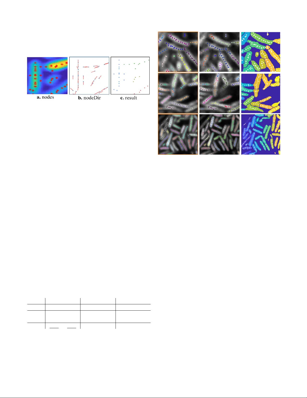
LCUTS: LINEAR CLUSTERING OF B A CTERIA USING RECURSIVE GRAPH CUTS J . W ang † , T . Batabyal † , M. Zhang ‡ , J . Zhang ‡ , A. Aziz ‡ , A. Gahlmann ‡ and S. T . Acton † † Department of Electrical & Computer Engineering and ‡ Department of Chemistry Uni versity of V irginia, Charlottesville, V A 22904, USA ABSTRA CT Bacterial biofilm segmentation poses significant challenges due to lack of apparent structure, poor imaging resolution, limited contrast between conterminous cells and high density of cells that o verlap. Although there e xist bacterial segmenta- tion algorithms in the existing art, they fail to delineate cells in dense biofilms, especially in 3D imaging scenarios in which the cells are growing and subdividing in a complex manner . A graph-based data clustering method, L Cuts, is presented with the application on bacterial cell segmentation. By con- structing a weighted graph with node features in locations and principal orientations, the proposed method can automatically classify and detect differently oriented aggregations of lin- ear structures (represent by bacteria in the application). The method assists in the assessment of sev eral facets, such as bacterium tracking, cluster growth, and mapping of migra- tion patterns of bacterial biofilms. Quantitativ e and qualita- tiv e measures for 2D data demonstrate the superiority of pro- posed method over the state of the art. Preliminary 3D results exhibit reliable classification of the cells with 97% accuracy . Index T erms — Segmentation, bacterial biofilm, cluster- ing, graph cut, point cloud data 1. INTR ODUCTION Analyzing cellular beha vior of indi vidual bacteria in a biofilm is a key for biologists and biochemists to understand biofilm growth, in div erse applications such as electrical power and public health research [1]. Lack of knowledge in macroscopic biofilm properties (e.g. size, shape, cohe- sion / adhesion) that emer ge from the behaviors of individual bacteria in different micro-en vironment is a major barrier in biofilm studies. T o make up for the deficiency , an advanced image analysis toolkit for segmenting indi vidual cells is in high demand along with ef ficient image acquisition methods, such as using super-resolution technology [2][3] that over - come the diffraction limit of traditional optical microsc opy techniques. The segmentation of indi vidual bacterial cells in dense bacterial biofilms is a challenging problem. One of the ma- jor challenges to the state of the art comes from the presence of inhomogeneous fluorescence intensity within a single cell Fig. 1 : Performance of L Cuts on 3D point cloud data comparing with manually grouped ground truth. The counting accuracy is 97% and grouping accuracy is 90% . Three viewpoints from left to right: 3D view , xy -plane and y z -plane. or across multiple cells. When using standard lev el set seg- mentation methods [4] and le vel sets using Legendre poly- nomials as basis functions [5], the segmentation fails where the contrast between the cells and background is weak. The watershed algorithm [6][7] uses the gradient flow to identify the morphological changes along segment contours, whereas [8] [9] separate large segments at the concavities. With both approaches, situations where the intensity of the regions of in- terest is non-homogeneous often lead to segmentation errors. Other edge-based parametric methods [10][11]are insufficient giv en the subtle and often absent boundaries between cells that are densely packed in three dimensions. T o achie ve 3D cell segmentation, the authors in [12] pre- sented a technique to track bacteria in a dense mono-layer by way of 3D time-lapse images. This solution employs an iterativ e threshold-based approach, which is heavily depen- dent on high contrast between the signal and background in the images. Y an et al . [13] proposed a single cell tracking toolkit based on marker controlled watershed and threshold techniques. This method allows tracking of bacterial growth in multi-layered biofilms when florescence intensity is uni- form and void spaces between cells are readily discernable, but struggles with the detection of individual bacteria when cells are closely packed or when inter- and intra-cellular flu- orescence intensity are not heterogeneous. Building on the work in [13], Hartmann et al . [14] recently reported a solu- tion to 3D segmentation in confocal images of biofilms that exploits prior knowledge of cell size to segment low density biofilms. As this method, like that of [13], is watershed- based, it suffers from similar drawbacks. In [15], the authors attempted to solve the problem via constructing single-cell re- gions to ensure the gap between neighboring cells in a seeded iterativ e active contour approach. The single cell identifica- tion performance degrades in the cases where the contrast be- tween cells and voids in the biofilm is lo w . As a solution to ov ercome the aforementioned limita- tions, namely the dif ficulty in segmenting dense aggregations in large biofilm with non-homogeneous inter- and intra-cell intensities, a novel approach is proposed in this paper with two major contrib utions: • The bacterial cell segmentation problem is transformed into a data clustering problem by generating pointillist data that represents the regions of interest; • A recursive multi-class linear data clustering algorithm ( L Cuts) is proposed that is capable of finding the lin- ear structures in point cloud data where cell boundaries may be ambiguous. Our approach is built on the following insight: Even though the raw image data does not show distinct boundaries in in- tensity between densely packed cells, we are still able to reli- ably compute local intensity maxima that delineate the central axis of each cell. Therefore, the proposed L Cuts algorithm first deriv es these maximal points and then partitions them based on the approximate co-linearity of points. Moreover , this local maximum-based initialization translates seamlessly and robustly into the 3D imaging and 3D segmentation prob- lem. 2. LINEAR CLUSTERING ALGORITHM Numerous algorithms exist in the clustering community that group the data by finding the similarities between classes. Distance, number of neighbors, density and predefined prob- ability distribution functions are the major perspectives for measuring similarities between points in the trending litera- ture, such as k-means [16], DBSCAN [17], DensityClust [18]. Among those, density based clustering methods ([17, 18]) de- tect non-spherical arbitrary clusters; howe ver , they are still limited in precisely classifying linear groups as discussed in the comparison in sec 3 . The Hough transform [19] is well known in detecting lines in the space, but the approach is not sufficient for delineating cells that are intersecting and is also computationally expensi ve. Unlike k-means and Densi- tyClust, our approach does not require manual intervention in order to locate appropriate number of clusters. Incorporation of structural constraints, such as the distance limit and the ec- centricity of the bacteria into L Cuts obviates the need for a priori information regarding the number of clusters (in our case, bacteria), making L Cuts a fully automatic approach. Fig. 2 : Intuitiv e work flow for the recursiv e program. Left: an example of bi-partition decision tree. Right: detailed example for checking the stopping criterion of component red. Here, siz eLimit , distLimit and eccLimit are parameters based on prior biological information. In the paper , we propose a recursiv e graph cuts algorithm (see work flo w in Fig. 2 ) for efficient computation to find the linear groups in the point cloud data. The algorithm can be primarily divided into three parts: construct the graph ( sec 2.1 ), compute the bi-partition solution, and recursi vely re- partition until the stopping criterion is satisfied ( sec 2.2 ). The bi-partition solution to separate the nodes (the local maxima) is inspired by [20]. They addressed the problem ”how to find the precise groups in an image” as normalized graph parti- tioning, where an image is partitioned into tw o groups, A and B , by disconnecting the edges between these two groups. 2.1. Graph construction Nodes: The nodes (local maxima along the ridgeline of a cell) in the constructed graph hav e two features: location ( nodeLoc ) and direction ( nodeD ir ). Location is simply the Cartesian position of the node. Direction of each node is the principal axis direction of the ridgeline computed via majority voting ( see Fig. 3 ). A ”neighborhood” consists of multi-hop neighbors that is constructed for voting. In graph theory , a ”hop” between two nodes is defined as the number of edges that one has to trav erse in order to reach from one node to the other node. Fig. 3 : An illustration of majority voting. (a) A 4-hop ”neighbor- hood” example. Each hop-neighbor is found within a specified dis- tance (dashed circles) to node. (b) The dashed lines connecting tar get node with all the other nodes in the neighborhood are possible ori- entations. (c) Those orientations that have larger relative angles with respect to the orientations are excluded from the candidates. (d) The direction to represent the target node is determined as the average orientation from the candidates. A N r × N p accumulator is set up for the majority v oting. One dimension of this accumulator represents the N p possible orientations ( p ) in N p bins (see Fig. 3b ). Another dimension corresponds to the quantized relati ve angles ( φ ) with N r bins, where φ is computed from each possible orientation to all the others. Here, N r is chosen based on the ”hop” number . The accumulator will count the number of parameter pairs ( p , φ ) that lie in each bin. W ithin the first bin of φ , the orientations with the largest value are selected which giv e the candidate directions. These candidates are av eraged to yield the major direction for the target node. Adjacency matrix: The adjacency matrix reflects the likelihood if two nodes are in the same group. Suppose there are N nodes in the graph, then the dimension of the adjacency matrix is N × N . Each attribute in the matrix represents the connectivity and edge weight between two nodes ( i , j ), which measures the similarity of their features according to: w ij = w distance · w direction · w intensity (1) Three similarity measures are in volv ed: the Euclidean dis- tance of locations of nodes ( eq 2 ), the relative angle between major directions ( eq 3 ) and the dissimilarity of intensity along the segment connecting two nodes ( eq 4 ). The first term is straightforward with an additional con- dition that sets the weights to be zero when two nodes are farther than a gi ven distance r (set by maximum cell length). w distance = ( e − D 2 ij /σ 2 D , if D ij ≤ r 0 , otherwise (2) where D ij = || nodeLoc i − nodeLoc j || 2 and σ D reflects the al- lowed variance for distance between nodes. The second part measures the angle difference between two node directions, called relative angle. Given two node directions, the relative angle ( θ ) is the cosine term that varies from 1 to 0 as θ be- comes larger . Then the corresponding weighting is giv en by: w direction = e − (cos( θ ) − 1) 2 /σ 2 T (3) By adjusting σ T , one can control the variance of relativ e an- gles within each group. The third term in (1) detects the intensity dissimilarity along the segment joining two nodes in the image, which is defined as: w intensity = ( min I i → j , if min I i → j ≤ thr esh 1 , otherwise (4) Here, thresh equals the difference between the midrange ( Mid ) of all the nodes and the variance ( V ar ) of the con- stituent node intensities. In the case that the nodes have no intensity information, this term can be set as 1 . Otherwise, we extract the intensities along the connecting segment from node i to node j from the image as shown in Fig. 4 and compute the lowest intensity along the segment and compare to thr esh . 2.2. Stopping criterion f or recursion T wo stopping conditions are checked after each bi- partition lev el to decide the completeness of the recursion. Fig. 4 : Illustration and motiv ation of defining intensity on edge weight. a : Nodes are denoted as red asterisk. b : After extracting the node directions from the red region in a , it is still hard to sep- arate two groups as the relativ e angle (in c ) and relativ e distance (shown in d, the distance is 10) are close. In this case, we ev aluate the intensity along the connection of the two nodes. The intensity changes are shown in d . The intensity weighting is then assigned as the lowest intensity lo wer than thr esh . Criterion 1 - size: The preliminary components that are less than siz eLimit have the potential to be an individual group. This siz eLimit is a user defined parameter . For the application we discuss in the paper , we used the prior bio- information of the maximum length of the bacterium to deter- mine the value. Criterion 2 - linearity: This criterion is designed for pre- serving the linear groups with different size from the poten- tials (after criterion 1). Intuitiv ely , if a single component is found (see black nodes in Fig. 2 ) and it is less than the maxi- mum size limit as specified, it may not be a finalized group as linearity remains to be checked. Three aspects are checked to ensure the linearity: (1) Standar d deviation ( Std ) from nodes in the group to the least square fitted line; (2) Intensity changes between the nodes within the group (as explained in Sec 2.1 ); (3) Eccentricity of the group. This is an optional condition based on the data type. For linear components, the eccentricity ( eccLimit ) is closer to 1; while, for circular com- ponents, it is closer to 0. 3. APPLICA TION AND ANAL YSIS 3.1. Experiments on bacterial images For qualitativ e and quantitati ve assessments, L Cuts is tested on 10 two-dimensional point cloud data which are generated from bacterial images using Airyscan microscopy . From these images, we obtain prior information regarding the longest bacterium in the dataset (approximately maximum 60 pixels in length and 15 pixels in width, where each pixel is 46 nm × 46 nm ). The typical data ha ve 250 to 600 nodes with approximately 20 to 60 cells observed. Fig. 5 : Pipeline for finding nodes from bacterial images. Step 1: Filter the original image with a Gaussian kernel (a → b). Step 2: Enhance the signals in the image via background subtraction (b → c). Step 3: Find the local maxima (c → d). Step 4: Clear the points if they hav e no neighbors or overlap with other points and rest are the found nodes (red asterisks in d). T o build the graph, we generate the point cloud data fol- lowing the pipeline in Fig. 5 . An experimental result and corresponding node features is shown in Fig . 6 . Fig. 6 : An example performance of L Cuts with constructed graph features. (a) Nodes are marked in red asterisks. (b) Red lines show the major direction features for each nodes (blue dots). (c) L Cut clustering results for the constructed graph. 3.2. Qualitative and quantitative comparison The performance of L Cuts is analyzed qualitatively and quantitativ ely by comparing with two current methods used in the bioimaging community , DensityClust [18] and Single Cell trac king [13]. Based on the imaging technique and bi- ological cell information, the parameter settings for L Cuts are siz eLimit = 60 pixels, distLimit = 5 pixels (maxi- mum distance between nodes that have neighborhood), and eccLimit = 0 . 9 . The parameters are also tuned in the other two algorithms to achiev e optimal performance in each case. In DensityClust , we chose ”Gaussian” mode for computing densities. Due to the manual input for the selection of cluster centers, we performed fiv e times for each data and chose the best performance from all. In Single Cell tracking , the wa- tershed value is the key to optimizing the algorithm, where a value of one is used. Qualitative comparison is sho wn in Fig. 7 . T wo measures, grouping accuracy (GAcc) and counting accuracy (CAcc), are computed for quantitativ e comparison using D ice = 2TP/(2TP + FP +FN), where T P = true posi- tiv e, F P = false positi ve, and F N = false negati ve. GAcc ac- counts for the performance of how many nodes are correctly classified in each group (cell); while CAcc indicates the clas- sification accuracy in terms of matching the final clusters with individual cells in the image. Here, indi vidual cell regions are manually labeled as ground truth in the comparison. L Cuts DensityClust SCT GAcc CAcc GAcc CAcc GAcc CAcc Best 95.9 95.1 94.6 92.3 94.4 94.1 W orst 87.8 85.2 78.3 83.7 77.8 53.5 A vg 91.6 91.2 85.9 87.2 87.7 86.5 T able 1 : Quantitativ e comparison of L Cuts with Density- Clust [18] and Single Cell T racking [13] using Dice scores. Overall, L Cuts outperforms DensityClust and SCT in GAcc and CAcc by a margin of at least 4 % on a verage. There are circumstances that some cells are misclassified in L Cuts. Fig. 7 : Qualitativ e comparison for proposed method (first column) with DensityClust [18] (second column) and Single Cell Tracking [13] (third column). For L Cuts and DensityClust, different groups are marked with different colors and sho wn on the original image. The results of Single Cell Tracking are shown by overlapping the point cloud data on the segmented image, where dif ferent colors rep- resent different single cell groups. One cause is the non-linearity of auto-produced point cloud data, especially when cells are randomly floating in the three- dimensional space. Another cause is the trade-off between the tolerance in distance/intensity changes and the continuity of the linear structure. L Cuts can be directly applied on three-dimensional data. A preliminary result is sho wn in Fig. 1 with a Counting Accu- racy of 97% . The point cloud data was generated by biofilm researchers in Gahlmann Lab . They manually labeled the cen- ters of each bacteria slice by slice from x , y and z directions in Lattice Lightsheet microscopic image. The ground truth was manually grouped which reflects the actual single bacterium layout in 3D space. 4. CONCLUSION W e presented L Cuts, a graph-based solution for finding linear structures in multi-dimensional spaces. L Cuts outper- forms the existing methods in majority of cases. Furthermore, L Cuts enables automated processing of 2D and 3D images to identify individual bacteria in biofilms independent of the number of bacteria present. L Cuts provides quantifiable in- formation in the form of cellular positions, orientations, and the physical contact points between them. Be yond bacterial biofilms, L Cuts can be extended to other biological applica- tions in which boundaries are elusiv e b ut ridgelines of objects are accessible. 5. REFERENCES [1] Carey D Nadell, Knut Drescher, and Kevin R Fos- ter , “Spatial structure, cooperation and competition in biofilms, ” Natur e Reviews Micr obiology , vol. 14, no. 9, pp. 589, 2016. [2] Andreas Gahlmann and WE Moerner , “Exploring bac- terial cell biology with single-molecule tracking and super-resolution imaging, ” Nature Reviews Micr obiol- ogy , v ol. 12, no. 1, pp. 9, 2014. [3] Steffen J Sahl, Stefan W Hell, and Stefan Jakobs, “Flu- orescence nanoscopy in cell biology , ” Natur e re views Molecular cell biology , v ol. 18, no. 11, pp. 685, 2017. [4] Scott T Acton and Nilanjan Ray , “Biomedical image analysis: Segmentation, ” Synthesis Lectures on Image, V ideo, and Multimedia Pr ocessing , vol. 4, no. 1, pp. 1– 108, 2009. [5] Suvadip Mukherjee and Scott T Acton, “Region based segmentation in presence of intensity inhomogeneity us- ing legendre polynomials, ” IEEE Signal Pr ocessing Let- ters , v ol. 22, no. 3, pp. 298–302, 2015. [6] Luc V incent and Pierre Soille, “W atersheds in digital spaces: an efficient algorithm based on immersion sim- ulations, ” IEEE T ransactions on P attern Analysis & Ma- chine Intelligence , , no. 6, pp. 583–598, 1991. [7] Anthony S Wright and Scott T Acton, “W atershed pyra- mids for edge detection, ” in IEEE International Confer- ence on Image Pr ocessing (ICIP) . IEEE, 1997, vol. 2, pp. 578–581. [8] Matthew A Reyer , Eric L McLean, Shriram Chennake- sav alu, and Jingyi Fei, “ An automated image analysis method for segmenting fluorescent bacteria in three di- mensions, ” Biochemistry , vol. 57, no. 2, pp. 209–215, 2017. [9] Y ong He, Hui Gong, Benyi Xiong, Xiaofeng Xu, Anan Li, T ao Jiang, Qingtao Sun, Simin W ang, Qingming Luo, and Shangbin Chen, “icut: an integrati ve cut algo- rithm enables accurate segmentation of touching cells, ” Scientific r eports , vol. 5, pp. 12089, 2015. [10] Nilanjan Ray and Scott T Acton, “ Activ e contours for cell tracking, ” in Image Analysis and Interpr etation, 2002. Pr oceedings. F ifth IEEE Southwest Symposium on . IEEE, 2002, pp. 274–278. [11] A-R Mansouri, Dipti Prasad Mukherjee, and Scott T Acton, “Constraining active contour ev olution via lie groups of transformation, ” IEEE T r ansactions on Image Pr ocessing , vol. 13, no. 6, pp. 853–863, 2004. [12] Sajith Kecheril Sadanandan, ¨ Ozden Baltekin, Klas EG Magnusson, Alexis Boucharin, Petter Ranefall, Joakim Jald ´ en, Johan Elf, and Carolina W ¨ ahlby , “Segmentation and track-analysis in time-lapse imaging of bacteria, ” IEEE Journal of Selected T opics in Signal Pr ocessing , vol. 10, no. 1, pp. 174–184, 2016. [13] Jing Y an, Andrew G Sharo, Ho ward A Stone, Ned S W ingreen, and Bonnie L Bassler , “V ibrio cholerae biofilm growth program and architecture rev ealed by single-cell liv e imaging, ” Pr oceedings of the National Academy of Sciences , v ol. 113, no. 36, pp. E5337– E5343, 2016. [14] Raimo Hartmann, Praveen K Singh, Philip Pearce, Rachel Mok, Boya Song, Francisco D ´ ıaz-Pascual, J ¨ orn Dunkel, and Knut Drescher , “Emergence of three- dimensional order and structure in growing biofilms, ” Natur e Physics , p. 1, 2018. [15] J W ang, R Sarkar , A Aziz, Andrea V accari, A Gahlmann, and Scott T Acton, “Bact-3d: A lev el set se gmentation approach for dense multi-layered 3d bacterial biofilms, ” in 2017 IEEE International Confer ence on Image Processing (ICIP) . IEEE, 2017, pp. 330–334. [16] James MacQueen et al., “Some methods for classifica- tion and analysis of multiv ariate observations, ” in Pr o- ceedings of the fifth Berkeley symposium on mathemati- cal statistics and pr obability . Oakland, CA, USA, 1967, vol. 1, pp. 281–297. [17] Martin Ester , Hans-Peter Kriegel, J ¨ org Sander , Xiaowei Xu, et al., “ A density-based algorithm for discovering clusters in large spatial databases with noise., ” in Kdd , 1996, vol. 96, pp. 226–231. [18] Alex Rodriguez and Alessandro Laio, “Clustering by fast search and find of density peaks, ” Science , v ol. 344, no. 6191, pp. 1492–1496, 2014. [19] Priyanka Mukhopadhyay and Bidyut B Chaudhuri, “ A surve y of hough transform, ” P attern Recognition , vol. 48, no. 3, pp. 993–1010, 2015. [20] Jianbo Shi and Jitendra Malik, “Normalized cuts and image segmentation, ” IEEE T ransactions on pattern analysis and machine intelligence , vol. 22, no. 8, pp. 888–905, 2000.