ASD-DiagNet: A hybrid learning approach for detection of Autism Spectrum Disorder using fMRI data
Mental disorders such as Autism Spectrum Disorders (ASD) are heterogeneous disorders that are notoriously difficult to diagnose, especially in children. The current psychiatric diagnostic process is based purely on the behavioural observation of symp…
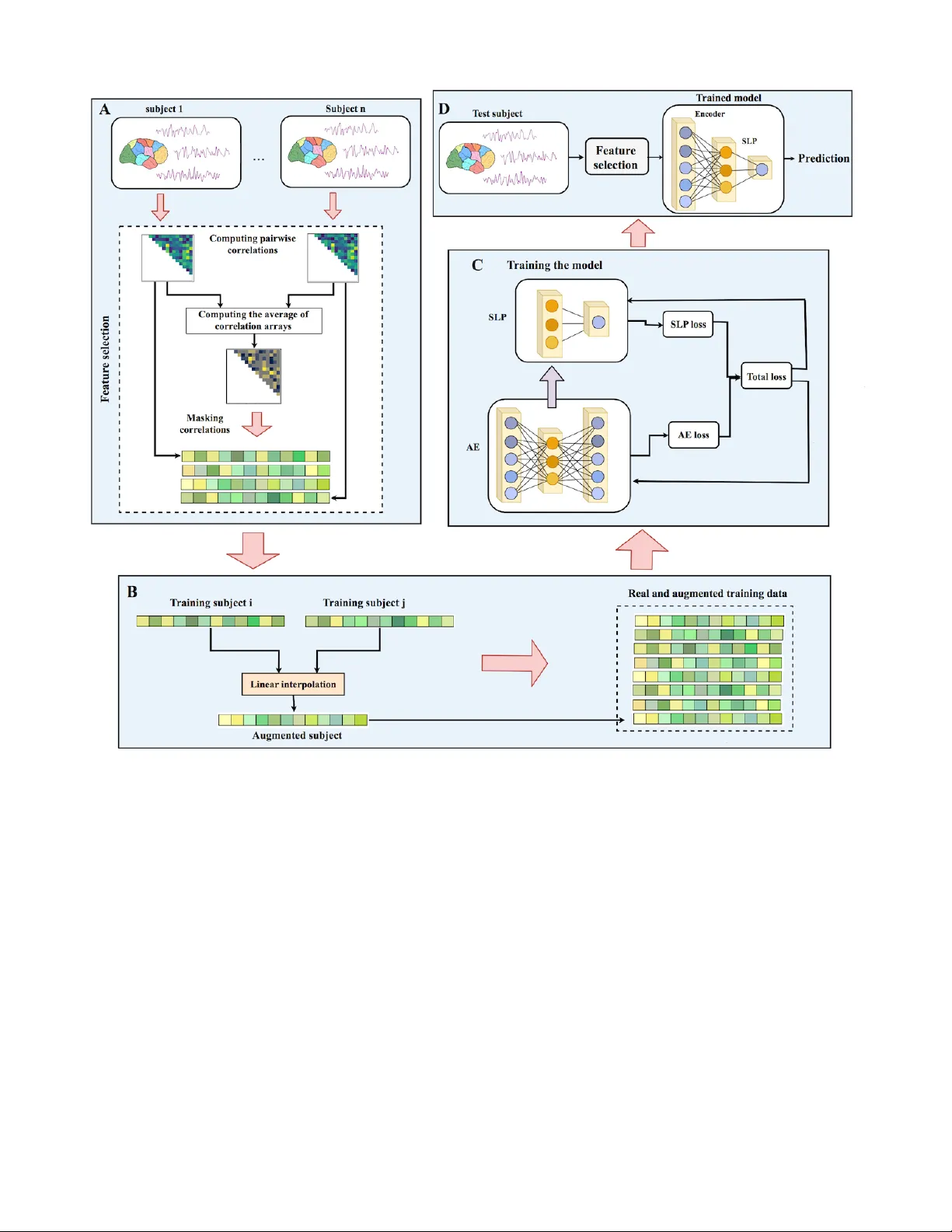
Authors: Taban Eslami, Vahid Mirjalili, Alvis Fong
1 ASD-DiagNet: A hybrid learning approach for detection of Autism Spectrum Disorder using fMRI data T aban Eslami, V ahid Mirjalili, Alvis Fong, Angela Laird, and F ahad Saeed ∗ , Abstract —Mental disorders such as A utism Spectrum Disor- ders (ASD) are heter ogeneous disorders that are notoriously dif- ficult to diagnose, especially in children. The current psychiatric diagnostic process is based purely on the behavioural observation of symptomology (DSM-5/ICD-10) and may be prone to over - prescribing of drugs due to misdiagnosis. In order to move the field towards more quantitative fashion, we need advanced and scalable machine learning infrastructure that will allow us to identify reliable biomarkers of mental health disorders. In this paper , we propose a framework called ASD-DiagNet for classifying subjects with ASD from healthy subjects by using only fMRI data. W e designed and implemented a joint learning pro- cedure using an autoencoder and a single layer perceptron which results in impro ved quality of extracted features and optimized parameters for the model. Further , we designed and implemented a data augmentation strategy , based on linear interpolation on av ailable feature vectors, that allows us to produce synthetic datasets needed for training of machine learning models. The proposed approach is evaluated on a public dataset provided by A utism Brain Imaging Data Exchange including 1035 subjects coming from 17 different brain imaging centers. Our machine learning model outperforms other state of the art methods from 13 imaging centers with increase in classification accuracy up to 20% with maximum accuracy of 80%. The machine learning technique presented in this paper , in addition to yielding better quality , gives enormous advantages in terms of execution time (40 minutes vs. 6 hours on other methods). The implemented code is a vailable as GPL license on GitHub portal of our lab (https://github .com/pcdslab/ASD-DiagNet). Index T erms —fMRI, ASD, SLP , A utoencoder , ABIDE, Classi- fication, Data augmentation I . I N T RO D U C T I O N M ENT AL disorders such as Autism Spectrum Disorders (ASD) are heterogeneous disorders that are notoriously difficult to diagnose, especially in children. The current psy- chiatric diagnostic process is based purely on behavioural observation of symptomology (DSM-5/ICD-10) and may be prone to misdiagnosis [1]. There is no quantitati ve test that can be prescribed to patients that may lead to definite diagnosis of a person. Such quantitativ e and definiti ve tests are a regular T . Eslami and A. Fong are with the Department of Computer Sci- ence, W estern Mihcigan univ ersity , Kalamazoo, MI, 49008. E-mail: ta- ban.eslami,alvis.fong@wmich.edu V . Mirjalili is with Department of Computer Science and Engineering, Michigan State University , Lansing, MI, 48824. E-mail: mirjalil@msu.edu A. Laird is with Department of Physics, Florida International University , Miami, FL, 33199. E-mail: alaird@fiu.edu F . Saeed is with school of computing and information science, Florida International Univ ersity , Miami, FL, 33199. ∗ Corresponding E-mail: fsaeed@fiu.edu practice for other diseases such as diabetes, HIV , and hepatitis- C. It is widely known that defining and diagnosing mental health disorders is a dif ficult process due to overlapping nature of symptoms, and lack of a biological test that can serve as a definite and quantified gold standard [2]. Autism Spectrum Disorders (ASD) is a lifelong neuro-developmental brain disorder which causes social impairments like repetitiv e behaviour and communication problems in children. More than 1% of children suffer from this disorder and detecting it at early ages can be beneficial. Studies show that some demographic attributes like gender and race vary among ASD and healthy indi viduals such that males are four times more prone to ASD than females [3]. Quantitativ e analysis of brain imaging data can provide valuable biomarkers that result in more accurate diagnosis of brain diseases. Machine learning techniques using brain imaging data (e.g. Magnetic Resonance Imaging (MRI) and functional Magnetic Resonance Imaging (fMRI)) hav e been extensi vely used by researchers for diagnosing brain disorders like Alzheimer’ s, ADHD, MCI and, Autism. [4], [5], [6], [7], [8], [9], [10]. In this paper , we focus on classifying subjects suf fering from Autism Spectrum Disorders (ASD) from healthy control subjects using fMRI data. W e propose a method called ASD- DiagNet which consists of an autoencoder and a single layer perceptron. These networks are used for extracting lower dimensional features in a hybrid manner and the trained perceptron is used for the final round of classification. In order to enlarge the size of the training set, we designed a data augmentation technique which generates new data in feature space by using available data in the training set. Based on the experimental results, ASD-DiagNet achieved 70 . 1% classification accuracy which outperforms the current state of the art technique [11]. Further , we show that ASD-DiagNet scales extremely well with increasing size of the data and takes only 41 minutes to run as compared to 6 hours needed by other methods [11]. A verage accuracy on individual sites is 63% , which is 7% better than the result reported by [11]. Our machine learning technique will allow greater quantification of ASD diagnosis and is a step forward to making the early diagnosis and treatment a priority . The structure of this paper is as follows: In the next section, we explain the state of the art in the field. In Section III, we explain ASD-DiagNet method in detail. In Section IV, we describe the experiment setting and discuss the results of ASD-DiagNet. Finally , in Section V, we conclude the paper 2 and discuss future direction. I I . B A C K G RO U N D I N F O R M A T I O N A N D L I T E R A T U R E R E V I E W Detecting ASD using fMRI data has recently gained a lot of attention, thanks to Autism Brain Imaging Data Exchange (ABIDE) initiati ve for providing functional and structural brain imaging datasets collected from se veral brain imaging centers around the world [12]. Many studies and methods ha ve been dev eloped based on ABIDE data [11], [13], [14], [15]. Some studies included a subset of this dataset based on specific demographic information to analyze their proposed method. For example, Iidaka [13] used probabilistic neural network for classifying resting state fMRI (rs-fMRI) data from 312 ASD and 328 healthy control subjects (Subjects under 20 years old were selected) which achie ved around 90% accuracy . In another work, Plit et al. [16] used two sets of rs-fMRI data, one containing 118 male individuals ( 59 ASD; 59 TD) and the other containing 178 age and IQ matched individuals ( 89 ASD; 89 TD) from ABIDE dataset and achieved 76 . 67% accuracy . Besides using fMRI data, some studies also included struc- tural and demographic information of subjects for diagnosing ASD. Parisot et al. [17] proposed a framew ork based on Graph Con volutional Netw orks that achiev ed 70 . 4% accuracy . In their work, they represented the population as a graph in which nodes are defined based on imaging features and phenotypic information describe the edge weights. Sen et al. [18] proposed a new algorithm which combines structural and functional features from MRI and fMRI data and got 64 . 3% accuracy by using 1111 total healthy and ASD subjects. Nielsen et al. [19] obtained 60% accuracy on a group of 964 healthy and ASD subjects using the functional connecti vity between 7266 regions and demographic information like age, gender, and handedness attributes. Machine learning techniques such as Support V ector Ma- chines (SVM) and Random Forests are explored in mul- tiple studies [20], [21], [15], [22]. For instance, Chen et al. [14] in vestigated the effect of different frequenc y bands for constructing brain functional network, and obtained 79 . 17% accuracy using SVM technique applied to 112 ASD and 128 healthy control subjects. Recently , using neural networks and deep learning methods such as autoencoders, Deep Neural Network (DNN), Long Short T erm Memory (LSTM) and Con volutional Neural Net- work (CNN) ha ve also become very popular for diagnosing ASD [23], [24], [25], [26], [27], [28]. Brown et al. [25] obtained 68 . 7% classification accuracy on 1013 subjects com- posed of 539 healthy control and 474 with ASD, by proposing an element-wise layer for deep neural networks which incor- porated the data-dri ven structural priors. Most recently , Heinsfeld et al. [11] used a deep learning based approach and achieved 70% accuracy for classifying 1035 subjects ( 505 ASD and 530 controls). They claimed this approach improved the state of the art technique. In their tech- nique, distinct pairwise Pearson’ s correlation coef ficients were considered as features. T wo stacked denoising autoencoders were first pre-trained in order to extract lower dimensional data. After training autoencoders, their weights were applied to a multi-layer perceptron classifier (fine-tuning process) which was used for the final classification. Howe ver , they also performed classification for each of the 17 sites included in ABIDE dataset separately , and the a verage accurac y is reported as 52% . The lo w performance on individual sites was justified to be due to the lack of enough training samples for intra-site training. Generally , most related studies for ASD diagnosis using machine learning techniques hav e only considered a subset of ABIDE dataset, or they have incorporated other information besides fMRI data in their model. There are few studies such as [11], which only used fMRI data without any assumption on demographic information and analyzed all the 1035 subjects in ABIDE dataset. T o the best of our knowledge [11] is currently state of the art technique for ASD diagnosis on whole ABIDE dataset, which we use as the baseline for ev aluating our proposed method. I I I . M A T E R I A L S A N D M E T H O D S A. Functional Magnetic Resonance Imaging and ABIDE dataset Functional Magnetic Resonance Imaging (fMRI) is a brain imaging technique that is used for studying brain activities [29], [30]. In fMRI data, the brain volume is represented by a group of small cubic elements called voxels. A time series is extracted from each voxel by keeping track of its activity over time. Scanning the brain using fMRI technology while the subject is resting is called resting state fMRI (rs- fMRI), which is widely used for analyzing brain disorders. In this study , we used preprocessed ABIDE-I dataset that is provided by the ABIDE initiativ e. This dataset consists of 1112 rs-fMRI data including ASD and healthy subjects collected from 17 dif ferent sites. W e used fMRI data of the same group of subjects which was used in [11]. This set consists of 505 subjects with ASD and 530 healthy control from all the 17 sites. T able I shows the class membership information for each site. ABIDE-I provided the av erage time series extracted from sev en sets of regions of interest (R OIs) based on seven different atlases which are preprocessed using four different pipelines. The data used in our experiments is preprocessed using C-P A C pipeline [12] and is parcellated into 200 functionally homogeneous regions generated using spatially constrained spectral clustering algorithm [31] (CC- 200). The preprocessing steps include slice time correction, motion correction, nuisance signal removal, lo w frequency drifts and voxel intensity normalization. It is worth mentioning that each site used dif ferent parameters and protocols for scanning the data. Parameters like repetition time (TR), echo time (TE), number of v oxels, number of volumes, openness or closeness of the eyes while scanning are different among sites. B. ASD-DiagNet: F eature extraction and classification Functional connectivity between brain regions is an im- portant concept in fMRI analysis and is sho wn to contain 3 T able I: Class membership information of ABIDE-I dataset for each individual site Site Caltech CMU KKI Leuven MaxMun NYU OHSU OLIN PITT SBL SDSU Stanford T rinity UCLA UM USM Y ale ASD 19 14 20 29 24 75 12 19 29 15 14 19 22 54 66 46 28 Healthy control 18 13 28 34 28 100 14 15 27 15 22 20 25 44 74 25 28 Figure 1: Structure of an autoencoder consisting of an encoder that recei ves the input data and encodes it into a lower dimensional representation at the bottleneck layer , and a decoder that reconstructs the original input from the bottleneck layer . discriminativ e patterns for fMRI classification. Among cor- relation measures, Pearson’ s correlation is mostly used for approximating the functional connectivity in fMRI data [32], [33], [34]. It shows the linear relationship between the time series of two different regions. Giv en two times series, u and v , each of length T , the Pearson’ s correlation can be computed using the follo wing equation: ρ u v = Í T t = 1 ( u t − ¯ u )( v t − ¯ v ) q Í T t = 1 ( u t − ¯ u ) 2 q Í T t = 1 ( v t − ¯ v ) 2 (1) where ¯ u and ¯ v are the mean of times series u and v , respectiv ely . Computing all pairwise correlations results in a correlation matrix C m × m where m is the number of time series (or regions). Due to the symmetric property of Pearson’ s correlation, we only considered the strictly upper triangle part of the correlation matrix. Since we used CC-200 atlas in which the brain is parcellated into m = 200 regions, there are m × ( m − 1 )/ 2 = 19900 distinct pairwise Pearson’ s correlations. In this regard, we selected half of the correlations comprising 1 / 4 largest and 1 / 4 smallest values and eliminated the rest. T o do so, we first compute the average of correlations among all subjects in training set and then pick the indices of the largest positiv e and negati ve values from averaged correlation array . W e then pick the correlations at those indices from each sample as our feature vector . Keeping half of the correlations and eliminating the rest reduces the size of input features by a factor of 2. There is no limitation of the number of high- and anti-correlations that should be kept. Removing more features results in higher computational efficiency as well as reducing the chance of overfitting, ho wev er removing too many features can also cause loosing important patterns. In order to further reduce the size of features, we used an autoencoder to extract a lower dimensional feature representa- tion. An autoencoder is a type of feed-forward neural network model, which first encodes its input x to a lower dimensional representation, h e nc = φ e nc ( x ) = τ ( W e nc x + b e nc ) (2) where τ is the hyperbolic tangent activ ation function ( T an h ), and W e nc and b e nc represent the weight matrix and the bias for the encoder . Then, the decoder reconstructs the original input data x 0 = φ d ec ( h e nc ) = W d ec h e nc + b d ec (3) where W d ec and b d ec are the weight matrix and bias for the decoder . In this work, we hav e designed an autoencoder with tied weights, which means W d ec = W > e nc . An autoencoder can be trained to minimize its reconstruction error , computed as the Mean Squared Error (MSE) between x and its reconstruction, x 0 . The choice of using autoencoder instead of other feature extraction techniques like PCA is its ability to reduce the dimensionality of features in a non-linear way . Structure of an autoencoder is sho wn in Fig. 1. The lo wer dimensional data generated during the encoding process contains useful patterns from the original input data with smaller size, and can be used as new features for classification. For the classification task, we used a single layer perceptron (SLP) which uses the bottleneck layer of the autoencoder , h e nc , as input, and computes the probability of a sample belonging to the ASD patient class using a sigmoid activ ation function, σ , f ( x ) = σ W sl p h e nc + b sl p = σ W sl p τ ( W e nc x + b e nc ) + b sl p (4) where W sl p and b sl p are the weight matrix and the bias for the SLP network. The SLP network can be trained by minimizing the Binary Cross Entrop y loss, H , using the ground-truth class label, y , and the estimated ASD probability for each sample, f ( x ) : H ( y , f ( x )) = − ( y × f ( x ) + ( 1 − y ) × ( 1 − f ( x )) ) (5) 4 Finally , the predicted class label is determined by thresholding the estimated probability ˆ y = ( 1 , if f ( x ) ≥ 0 . 5 , 0 , otherwise . (6) T ypically , an autoencoder is fully trained such that its reconstruction error is minimized, then, the features from bottleneck layer , h e nc , are used as input for training the SLP classifier , separately . In contrast, here, we train the autoencoder and the SLP classifier simultaneously . This can potentially result in obtaining low dimensional features that hav e two properties 1) useful for reconstructing the original data, 2) contain discriminati ve information for the classification task. This is accomplished by adding the two loss functions, i.e. MSE loss for reconstruction, and Binary Cross Entropy for the classification task, and training both networks jointly . After the joint training process is completed, we further fine-tune the SLP network for a fe w additional epochs, while parameters of the autoencoder are frozen. C. Data augmentation using linear interpolation Machine learning and especially deep learning techniques can be advantageous if they are provided with enough training data. Insuf ficient data causes overfitting and non- generalizability of the model [35]. Large training sets are not always available and collecting new data might be costly like in medical imaging field. In these situations, data augmentation techniques can be used for generating synthetic data using the av ailable training set [36], [37], [38], [39], [40]. The data augmentation technique that we propose in this study is inspired by Synthetic Minority Over -sampling T echnique (SMO TE) [41]. SMO TE is an ef fectiv e model which is used for ov ersampling the data in minority class of imbalanced datasets. SMO TE generates synthetic data in feature space by using the nearest neighbors of a sample. After k-nearest neighbors of sample p are found ( { q 1 , q 2 , . . . , q k } ), a random neighbor is selected ( q r ) and the synthetic feature vector is computed using the follo wing equation: p 0 = α × p + ( 1 − α ) × q r (7) In this equation, α is a random number selected uniformly in the range [ 0 , 1 ] . In our implementation, we chose α randomly within range [ 0 . 5 , 1 ] , so that the synthesized sample is closer to p . Finding the nearest neighbors of a sample is based on a distance or similarity metric. In our work, the samples hav e feature vectors of size 9950 (half of the correlations). One idea for computing nearest neighbors is to use Euclidean distance, howe ver , computing the pairwise Euclidean distances with 9950 features is not ef ficient. In order to compute the similarity between samples and finding the nearest neighbors, we used a measure called Extended Frobenius Norm (ER OS). This mea- sure computes the similarity between two multiv ariate time series (MTS) [42]. fMRI data consists of sev eral regions each having a time series so we can consider it as a multiv ariate time series. Our previous study on ADHD disorder has sho wn that ER OS is an ef fectiv e similarity measure for fMRI data and using it along with k-Nearest-Neighbor achiev es high classification accuracy [5]. This motiv ated us to utilize it as part of the data augmentation process. EROS computes the similarities between two MTS items A and B based on eigen values and eigen vectors of their covariance matrices using the follo wing equation: E RO S ( A , B , w ) = Í n i = 1 w i | h a i , b i i | = Í n i = 1 w i | c os θ i | (8) where, θ i is the cosine of the angle between i t h correspond- ing eigen vectors of covariance matrices of multiv ariate time series A and B . Furthermore, w is the weight vector which is computed based on eigen values of all MTS items using Algorithm 1. This algorithm computes the weight vector w by normalizing eigen values of each MTS item followed by applying an aggregate function f (here, we used mean) to all eigen values ov er the entire training dataset and finally normalizing them so that Í n i = 1 w i = 1 . Algorithm 1 Computing weight vector for EROS [42] Input: An n × N matrix S , where n is the number of variables for the dataset and N is the number of MTS items in the dataset. Each column vector s i in S represents all the eigen values for i t h MTS item in the dataset. s i j is a v alue at column i and row j in S . s ∗ i is i t h row in S . s i ∗ is i t h column 1: for i = 1 to N do 2: s i ← s i / Í n j = 1 s i j 3: end for 4: for i = 1 to n do 5: w i ← f ( s ∗ i ) 6: end for 7: for i = 1 to n do 8: w i ← w i / Í n j = 1 w j 9: end for In order to further reduce the time needed for computing the pairwise similarities, we considered using the first two eigen vectors of each sample. Our experiments sho wed that this simplification does not af fect the results while reducing the running time significantly compared to using all eigen vectors and eigen values. Now , using EROS as the similarity measure, our data augmentation process is shown in Algorithm 2. After finding k = 5 nearest neighbors of each sample i in the training set, one of them is randomly selected, a new sample is generated using linear interpolation between the selected neighbor and sample i . Using this approach, one synthetic sample is created for each training point which results in doubling the size of the training set. Fig. 2 shows the data augmentation process and Fig. 3 shows the o verall process of ASD-DiagNet method. I V . E X P E R I M E N T S A N D R E S U LT S For all the experiments reported in this section, we used a Linux server running Ubuntu Operating System. The server 5 Figure 2: Generating new artificial data: Step 1) Selecting a sample ( p ). Step 2) Find k -nearest neighbors of p from the same class, and pick one random neighbor ( q r ). 3) Generate ne w sample p 0 using p and q r by linear interpolation. Algorithm 2 Data augmentation using ER OS similarity mea- sure Input: Training dataset of size N 1: for i = 1 to N do 2: Find 5 nearest neighbors to i using EROS 3: j ← A random sample among nearest neighbors 4: r ← Random number in the range [ 0 . 5 , 1 ] 5: x ∗ i + N ← α × x i + ( 1 − α ) × x j 6: end for contains two Intel Xeon E5-2620 Processors at 2 . 40 GHz with a total 48 GBs of RAM. The system contains an NVIDIA T esla K-40c GPU with 2880 CUDA cores and 12 GBs of RAM. CUDA version 8 and PyT orch library were used for conducting the experiments. W e ev aluated ASD-DiagNet model in two phases. In the first phase, the model was ev aluated using the whole 1035 subjects from all sites and in the second phase, the model was ev aluated for each site separately . As stated earlier , data centers may have used different experimental parameters for scanning fMRI images, so considering all of them in the same pool determines ho w our model generalizes to data with heterogeneous scanning parameters. On the other hand, by considering each data center separately , fewer subjects are av ailable for training the model and the results indicate how it performs on small datasets. In each of these experiments, the ef fect of data augmentation was ev aluated. The following subsections explain each experiment in more details. A. Phase 1: Experiments using the whole dataset In this phase, we performed 10-fold cross-validation on the whole 1035 subjects. T able II compares accuracy , sensitivity , and specificity of our approach with the method proposed by Heinsfeld et al. [11], random forest, and SVM with RBF kernel classifier . SVM and random forest were trained using 19900 pairwise Pearson’ s correlations for each subject. As the results show , ASD-DiagNet achie ves 70 . 1% which outperforms other methods. The proposed data augmentation helps to improv e the results by around 1% . 1 T able II: Classification performance using 10-fold cross- validation on the whole dataset; Note that our proposed approach, ASD-DiagNet (with data augmentation) achieves highest accuracy among existing methods. Method Accuracy Sensitivity Specificity ASD-DiagNet 70.1 67.8 72.8 ASD-DiagNet (no aug.) 69.2 66.4 73.1 SVM 60.3 35 84.4 Random F orest 63 54.9 71.3 Heinsfeild et al. [11] 65.4 69.3 61 B. Phase 2: Intra-site evaluation In this phase, we performed 5-Fold cross-validation on each site, separately . The accuracy of each method is provided in T able III. Based on these results, our method achiev es the highest accuracy in most cases and outperforms other methods on av erage. In addition, note that the proposed data augmentation helps impro ving the result around 2% overall. Especially , for OHSU, the data augmentation improv es the accuracy significantly ( 15% increase). C. Running time The running time needed for performing 10-fold cross- validation by different approaches is shown in T able IV. The training and ev aluation for all methods are performed on the same Linux system (described in Section IV). T able IV: Running time for 10-fold cross-validation (training and e valuation) on the whole dataset. Method Running time ASD-DiagNet 41 . 14 min ASD-DiagNet (no aug.) 20 . 5 min SVM 3 min Random forest 1 min Heinsfeild et al [11] 6 hr 1 W e like to mention that Heinsfeild [11] reported 70% accuracy in their paper , howe ver , the accuracy we reported here is the result of running their method on our system using their default parameters and the code they provided online. The different results observed here could be due to some missing details in the implementation. 6 Figure 3: W orkflow of ASD-DiagNet: A) Pairwise Pearson’ s correlations for each subject in the training set is computed. The av erage of all correlation arrays is computed and the position of 1 / 4 largest and 1 / 4 smallest values in the av erage array is considered as a mask. Masked correlation array of each sample is considered as its feature v ectors. B) A set of artificial samples is generated using the feature vectors of training samples. C) Autoencoder and SLP are jointly trained by adding up their training loss in each iteration. D) For a test subject, the features are extracted using the mask generated in part A, followed by passing the features through the encoder part of the autoencoder , and finally predicting its label using the trained SLP . Based on the results in T able IV, ASD-DiagNet performs significantly faster than [11]. The data augmentation doubles the size of the training set by generating one artificial sample per subject in the training set. As a result, the data augmen- tation increases the computation time by a factor of 2 . D. Experiment on other parcellations W e tested ASD-DiagNet on two other R OI atlases besides CC-200. The first parcellation is based on Automated Anatom- ical Labeling (AAL) atlas in which the brain is parcellated into 116 regions using AAL toolbox. The other atlas is called Dosenbach160 which parcellates the brain into 160 regions. The data for these parcellations is also provided in ABIDE dataset. Dosenbach160 and AAL contain 12720 and 6670 pairwise correlations, respecti vely . Similar to CC-200 atlas, half of the correlations (keeping the 1/4 largest and 1/4 smallest values, and removing the rest intermediate values) are selected as input features to the model. The resulting av erage accuracy , sensitivity , and specificity of performing 10-fold cross-validation on the whole dataset using different approaches for AAL and Dosenbakh160 are shown in T able V. 7 T able III: Classification accuracy using 5-fold cross-v alidation on individual data centers using our proposed method, ASD- DiagNet (with and without data augmentation), compared with other existing methods. Site ASD-DiagNet ASD-DiagNet Ref. [11] SVM Random- (no aug.) Forest Caltech 51.4 49.2 52.3 48.5 55.4 CMU 63.6 62.5 45.3 60 64.6 KKI 70.6 66.6 58.2 58.2 67.6 Leuven 59 57.2 51.8 53.9 57.5 MaxMun 48.3 48 54.3 53.8 45.8 NYU 68.5 66.1 64.5 57.1 62.3 OHSU 80 65.33 74 54 54.4 Olin 64.7 61.33 44 55.7 53.4 Pitt 68 66.8 59.8 51.8 60.87 SBL 53 52.3 46.6 50 47.6 SDSU 63.9 63 63.6 61.1 61.9 Stanford 62.5 61.5 48.5 51.4 60.1 T rinity 52.9 53.3 61 53.3 52.6 UCLA 72 71.3 57.7 55.1 69.3 USM 69 64 62 64.7 64.7 UM 64.2 64.7 57.6 52.8 63.5 Y ale 63.2 61.3 53 57.6 58.2 A verage 63.2 60.8 56.1 55.1 59.8 T able V: Classification accuracy using other parcellations of brain fMRI data: AAL and Dosenbach160; Note that our pro- posed method, ASD-DiagNet, outperforms existing techniques using both atlases. Method AAL Dosenbach160 ASD-DiagNet 67.8 65 ASD-DiagNet (no augmentation) 65.6 64.3 Heinsfeild et al [11] 65.8 63.8 SVM 59.3 51.7 Random forest 62.6 58.6 Based on the results in T able V, our proposed method with and without the augmentation process performs better than e x- isting methods. Note that the classification accuracy obtained using these parcellations are belo w the accurac y obtained using CC-200 atlas, which implies that the pairwise correlations among CC-200 regions contain more discriminativ e patterns than AAL and Dosenbakh160 atlases. V . C O N C L U S I O N A N D F U T U R E W O R K In this paper , we targeted the problem on classifying subjects with ASD disorder from healthy subjects. W e used fMRI data provided by ABIDE consortium, which has been collected from dif ferent brain imaging centers. No assumption or utilization of any demographic information is considered in this study . Our approach, called ASD-DiagNet , is based on using the most correlated and anti-correlated connections of the brain as feature vectors and using an autoencoder to extract lower dimensional patterns from them. The autoencoder and a single layer perceptron are trained in a joint approach for per- forming feature selection and classification. W e also proposed a data augmentation method in order to increase the number of samples using the a vailable training set. W e tested this method by performing 10-fold cross-v alidation on the whole dataset and achieved 70 . 1 % accuracy in 40 minutes. The running time of our approach is significantly shorter than 6 hours needed by the state of the art method while achie ving higher classification accuracy . In another experiment, we e valuated our method by performing 5-fold cross-validation on each data center , separately . The av erage result sho ws significant improvement in accuracy compared to the state of the art method. In this case, data augmentation helps to improve the accuracy by around 2 %. These results demonstrate that our approach can be used for both intra-site brain imaging data, which are usually small sets generated in research centers, and bigger multi-site datasets like ABIDE in a reasonable amount of time. F U N D I N G This research was supported by National Institute of General Medical Sciences (NIGMS), NIH A ward Number R15GM120820, and National Science F oundations (NSF) under A ward Numbers NSF CRII CCF-1464268, NSF CRII CCF- 1855441, NSF CAREER A CI-1651724 and NSF OA C 1925960. The content is solely the responsibility of the au- thors and does not necessarily represent the of ficial views of gov ernmental agencies. R E F E R E N C E S [1] R. E. Nickel and L. Huang-Storms, “Early identification of young chil- dren with autism spectrum disorder , ” The Indian Journal of P ediatrics , vol. 84, no. 1, pp. 53–60, 2017. [2] “ Attention deficit hyperactivity disorder: diagnosis and management of ADHD in children, young people and adults. ” National Collaborating Centre for Mental Health (UK), British Psychological Society , 2018. [3] J. Baio, L. Wiggins, D. L. Christensen, M. J. Maenner , J. Daniels, Z. W arren, M. Kurzius-Spencer , W . Zahorodny , C. R. Rosenberg, T . White et al. , “Prevalence of autism spectrum disorder among chil- dren aged 8 years—autism and dev elopmental disabilities monitoring network, 11 sites, united states, 2014, ” MMWR Surveillance Summaries , vol. 67, no. 6, p. 1, 2018. [4] E. Hosseini-Asl, G. Gimel’farb, and A. El-Baz, “ Alzheimer’s disease diagnostics by a deeply supervised adaptable 3D con volutional network, ” arXiv pr eprint arXiv:1607.00556 , 2016. [5] T . Eslami and F . Saeed, “Similarity based classification of ADHD using singular value decomposition, ” in Pr oceedings of the ACM International Confer ence on Computing F rontier s 2018 . A CM, 2018, pp. 19–25. [6] A. Khazaee, A. Ebrahimzadeh, A. Babajani-Feremi, A. D. N. Initiati ve et al. , “Classification of patients with MCI and AD from health y controls using directed graph measures of resting-state fMRI, ” Behavioural brain r esear ch , vol. 322, pp. 339–350, 2017. [7] Z. Y ang, S. Zhong, A. Carass, S. H. Y ing, and J. L. Prince, “Deep learn- ing for cerebellar ataxia classification and functional score regression, ” in International W orkshop on Machine Learning in Medical Imaging . Springer , 2014, pp. 68–76. [8] X. Peng, P . Lin, T . Zhang, and J. W ang, “Extreme learning machine- based classification of adhd using brain structural mri data, ” PloS one , vol. 8, no. 11, p. e79476, 2013. [9] J. B. Colby , J. D. Rudie, J. A. Brown, P . K. Douglas, M. S. Cohen, and Z. Shehzad, “Insights into multimodal imaging classification of ADHD, ” F rontier s in systems neur oscience , v ol. 6, p. 59, 2012. [10] G. Deshpande, P . W ang, D. Rangaprakash, and B. W ilamowski, “Fully connected cascade artificial neural network architecture for attention deficit hyperactivity disorder classification from functional magnetic resonance imaging data, ” IEEE transactions on cybernetics , v ol. 45, no. 12, pp. 2668–2679, 2015. [11] A. S. Heinsfeld, A. R. Franco, R. C. Craddock, A. Buchweitz, and F . Meneguzzi, “Identification of autism spectrum disorder using deep learning and the abide dataset, ” Neur oImage: Clinical , vol. 17, pp. 16– 23, 2018. 8 [12] C. Craddock, Y . Benhajali, C. Chu, F . Chouinard, A. Evans, A. Jakab, B. S. Khundrakpam, J. D. Lewis, Q. Li, M. Milham et al. , “The neuro bureau preprocessing initiativ e: open sharing of preprocessed neuroimaging data and deriv atives, ” Neur oinformatics , 2013. [13] T . Iidaka, “Resting state functional magnetic resonance imaging and neural network classified autism and control, ” Cortex , v ol. 63, pp. 55– 67, 2015. [14] H. Chen, X. Duan, F . Liu, F . Lu, X. Ma, Y . Zhang, L. Q. Uddin, and H. Chen, “Multiv ariate classification of autism spectrum disorder using frequency-specific resting-state functional connectivity—a multi- center study , ” Pro gress in Neuro-Psyc hopharmacology and Biological Psychiatry , vol. 64, pp. 1–9, 2016. [15] A. Abraham, M. P . Milham, A. Di Martino, R. C. Craddock, D. Samaras, B. Thirion, and G. V aroquaux, “Deri ving reproducible biomarkers from multi-site resting-state data: An autism-based example, ” Neur oImage , vol. 147, pp. 736–745, 2017. [16] M. Plitt, K. A. Barnes, and A. Martin, “Functional connectivity clas- sification of autism identifies highly predictive brain features but falls short of biomarker standards, ” NeuroImag e: Clinical , vol. 7, pp. 359– 366, 2015. [17] S. Parisot, S. I. Ktena, E. Ferrante, M. Lee, R. Guerrero, B. Glocker , and D. Rueckert, “Disease prediction using graph con volutional networks: Application to autism spectrum disorder and alzheimer’ s disease, ” Med- ical imag e analysis , 2018. [18] B. Sen, N. C. Borle, R. Greiner , and M. R. Brown, “ A general prediction model for the detection of ADHD and autism using structural and functional MRI, ” PloS one , vol. 13, no. 4, p. e0194856, 2018. [19] J. A. Nielsen, B. A. Zielinski, P . T . Fletcher , A. L. Alexander , N. Lange, E. D. Bigler, J. E. Lainhart, and J. S. Anderson, “Multisite functional connectivity MRI classification of autism: Abide results, ” F r ontiers in human neur oscience , vol. 7, p. 599, 2013. [20] V . Subbaraju, M. B. Suresh, S. Sundaram, and S. Narasimhan, “Identi- fying differences in brain activities and an accurate detection of autism spectrum disorder using resting state functional-magnetic resonance imaging: A spatial filtering approach, ” Medical image analysis , vol. 35, pp. 375–389, 2017. [21] A. J. Fredo, A. Jahedi, M. Reiter, and R.-A. Müller , “Diagnostic classification of autism using resting-state fMRI data and conditional random forest, ” Age (years) , vol. 12, no. 2.76, pp. 6–41, 2018. [22] X.-a. Bi, Y . W ang, Q. Shu, Q. Sun, and Q. Xu, “Classification of autism spectrum disorder using random support vector machine cluster, ” F rontier s in genetics , vol. 9, p. 18, 2018. [23] X. Guo, K. C. Dominick, A. A. Minai, H. Li, C. A. Erickson, and L. J. Lu, “Diagnosing autism spectrum disorder from brain resting-state functional connecti vity patterns using a deep neural netw ork with a nov el feature selection method, ” F rontier s in neur oscience , vol. 11, p. 460, 2017. [24] X.-a. Bi, Y . Liu, Q. Jiang, Q. Shu, Q. Sun, and J. Dai, “The diagnosis of autism spectrum disorder based on the random neural network cluster , ” F rontier s in human neur oscience , v ol. 12, p. 257, 2018. [25] C. J. Brown, J. Kawahara, and G. Hamarneh, “Connectome priors in deep neural networks to predict autism, ” in Biomedical Imaging (ISBI 2018), 2018 IEEE 15th International Symposium on . IEEE, 2018, pp. 110–113. [26] N. C. Dvornek, P . V entola, K. A. Pelphrey , and J. S. Duncan, “Iden- tifying autism from resting-state fMRI using long short-term memory networks, ” in International W orkshop on Machine Learning in Medical Imaging . Springer , 2017, pp. 362–370. [27] H. Li, N. A. Parikh, and L. He, “ A nov el transfer learning approach to enhance deep neural network classification of brain functional connec- tomes, ” F r ontiers in neur oscience , vol. 12, p. 491, 2018. [28] M. Khosla, K. Jamison, A. Kuceyeski, and M. Sabuncu, “3D con vo- lutional neural networks for classification of functional connectomes, ” arXiv pr eprint arXiv:1806.04209 , 2018. [29] M. A. Lindquist et al. , “The statistical analysis of fMRI data, ” Statistical science , v ol. 23, no. 4, pp. 439–464, 2008. [30] T . Eslami and F . Saeed, “Fast-GPU-PCC: A GPU-based technique to compute pairwise pearson’s correlation coefficients for time series data—fMRI study , ” High-thr oughput , vol. 7, no. 2, p. 11, 2018. [31] R. C. Craddock, G. A. James, P . E. Holtzheimer III, X. P . Hu, and H. S. Mayberg, “ A whole brain fMRI atlas generated via spatially constrained spectral clustering, ” Human brain mapping , vol. 33, no. 8, pp. 1914– 1928, 2012. [32] X. Liang, J. W ang, C. Y an, N. Shu, K. Xu, G. Gong, and Y . He, “Effects of different correlation metrics and preprocessing factors on small-world brain functional networks: a resting-state functional MRI study , ” PloS one , v ol. 7, no. 3, p. e32766, 2012. [33] Y . Zhang, H. Zhang, X. Chen, S.-W . Lee, and D. Shen, “Hybrid high- order functional connectivity networks using resting-state functional MRI for mild cognitive impairment diagnosis, ” Scientific reports , vol. 7, no. 1, p. 6530, 2017. [34] H.-C. Baggio, R. Sala-Llonch, B. Segura, M.-J. Marti, F . V alldeoriola, Y . Compta, E. T olosa, and C. Junqué, “Functional brain networks and cognitiv e deficits in parkinson’ s disease, ” Human br ain mapping , v ol. 35, no. 9, pp. 4620–4634, 2014. [35] S. Raschka and V . Mirjalili, Python machine learning . Packt Publishing Ltd, 2017. [36] S. C. W ong, A. Gatt, V . Stamatescu, and M. D. McDonnell, “Understand- ing data augmentation for classification: when to warp?” arXiv preprint arXiv:1609.08764 , 2016. [37] L. Perez and J. W ang, “The effectiv eness of data augmentation in image classification using deep learning, ” arXiv pr eprint arXiv:1712.04621 , 2017. [38] A. Eitel, J. T . Springenberg, L. Spinello, M. Riedmiller, and W . Burgard, “Multimodal deep learning for robust RGB-D object recognition, ” in Intelligent Robots and Systems (IROS), 2015 IEEE/RSJ International Confer ence on . IEEE, 2015, pp. 681–687. [39] A. Karpathy , G. T oderici, S. Shetty , T . Leung, R. Sukthankar , and L. Fei-Fei, “Large-scale video classification with conv olutional neural networks, ” in Pr oceedings of the IEEE conference on Computer V ision and P attern Recognition , 2014, pp. 1725–1732. [40] Y . Xu, R. Jia, L. Mou, G. Li, Y . Chen, Y . Lu, and Z. Jin, “Improved relation classification by deep recurrent neural networks with data augmentation, ” arXiv preprint , 2016. [41] N. V . Chawla, K. W . Bowyer , L. O. Hall, and W . P . Kegelme yer , “SMO TE: synthetic minority over -sampling technique, ” Journal of arti- ficial intelligence resear ch , vol. 16, pp. 321–357, 2002. [42] K. Y ang and C. Shahabi, “ A PCA-based similarity measure for multi vari- ate time series, ” in Proceedings of the 2nd A CM international workshop on Multimedia databases . ACM, 2004, pp. 65–74.
Original Paper
Loading high-quality paper...
Comments & Academic Discussion
Loading comments...
Leave a Comment