Tracking Multiple Audio Sources with the von Mises Distribution and Variational EM

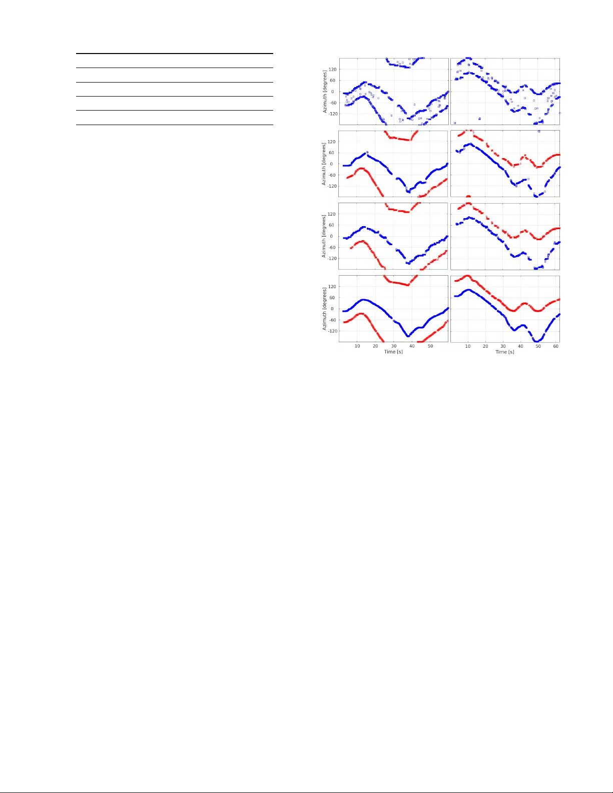
1 T racking Multiple Audio Sources with the v on Mises Distrib ution and V ariational EM Y utong Ban, 1 Xavier Alameda-Pineda, 1 Senior Member , IEEE , Christine Evers, 2 Senior Member , IEEE , and Radu Horaud 1 Abstract —In this paper we address the problem of simul- taneously tracking several moving audio sources, namely the problem of estimating source trajectories from a sequence of observed features. W e propose to use the von Mises distribution to model audio-source directions of arriv al with circular random variables. This leads to a Bayesian filtering formulation which is intractable because of the combinatorial explosion of associating observed variables with latent variables, over time. W e propose a variational approximation of the filtering distrib ution. W e infer a variational expectation-maximization algorithm that is both computationally tractable and time efficient. W e propose an audio-source birth method that favors smooth sour ce trajectories and which is used both to initialize the number of active sources and to detect new sources. W e perf orm experiments with the recently released LOCA T A dataset comprising two moving sources and a moving microphone array mounted onto a robot. Index T erms —Multiple target tracking, Bayesian filtering, von Mises distribution, variational approximation, EM. I . I N T RO D U C T I O N W e address the problem of tracking several moving audio sources. Audio tracking is useful for audio-source separation, spatial filtering, speaker diarization, speech enhancement and speech recognition, which in turn are essential methodologies, e.g. home assistants. Audio-source tracking is dif ficult because audio signals are adv ersely affected by noise, re verberation and interferences between acoustic signals. Single-source tracking methods are based on observing time differences of arri val (TDO As) between microphones. Since the mapping between TDOAs and the source locations is non- linear , sequential Monte Carlo approaches are used, e.g. [1]– [3]. Alternativ ely , directions of arriv al (DO As) can be used. The problem is cast into a linear dynamic model, e.g. [4]. In this case source directions should howe ver be modeled as cir- cular random variables, e.g. the wrapped Gaussian distribution [5], or the von Mises distribution [6], [7]. Multiple-source tracking is more challenging: (i) the number of activ e sources is unknown and v aries over time, (ii) sev eral DO As need be detected, and (iii) DOA-to-source assignments must be estimated. An unknown number of sources was addressed using random finite sets [8]. Since the probability 1 Y . Ban, X. Alameda-Pineda and R. Horaud are with Inria Grenoble Rh ˆ one- Alpes, Montbonnot Saint-Martin, France. E-mail: first.last@inria.fr 2 C. Evers is with Dept. Electrical and Electronic Engineering, Im- perial College London, Exhibition Road, SW7 2AZ, UK. Email: c.evers@imperial.ac.uk This work was supported by the ERC Adv anced Grant VHIA #340113 and the UK EPSRC Fello wship grant no. EP/P001017/1. density function (pdf) is computationally intractable, its first- order approximation can be propagated in time using the probability hypothesis density (PHD) filter [8], [9]. In [10] the PHD filter was applied to audio recordings to track multiple sources from TDOA estimates. In [11] the wrapped Gaussian distribution is incorporated within a PHD filter . The von Mises-Fisher distribution was used in [12] to build a factorial filter . A mixture of v on Mises distributions was combined with a PHD filter in [13]. The main drawback of PHD filters is that explicit observ ation-to-source associations are not established. Instead, post-processing techniques are required for track labelling [14]. A v ariational approximation of the multiple target track- ing was addressed in [15]: bservation-to-tar get associations are discrete latent v ariables which are estimated with an variational expectation maximization (VEM) solver . More- ov er, the problem of tracking a varying number of targets is addressed via track-birth and track-death processes. The variational approximation of [15] was recently extended to track multiple speakers with audio [16] and audio-visual data [17]. This paper builds on [7], [15], [16] and proposes to use the von Mises distribution to model the DOAs of multiple acoustic sources with circular random v ariables. The Bayesian filtering formulation for the multi-source tracking problem is intractable over time, due to the combinatorial nature of the unknown association between observed v ariables and latent variables. W e propose a variational approximation of the filtering distribution. A nov el mathematical framew ork is therefore proposed in order to deal with a mixture of von Mises distributions. The contribution of this paper is therefore a novel VEM algorithm that is both computationally tractable and time ef ficient. Moreov er, we propose an audio-source birth method that fa vors smooth source trajectories and which is used both to initialize the number of activ e sources and to detect ne w sources. W e perform experiments with the recently released LOCA T A dataset [18] comprising audio recordings of two moving sources from a moving microphone array in a real acoustic environment. The paper is org anized as follows. Section II describes the probabilistic model and Section III describes a vari- ational approximation of the filtering distribution and the VEM algorithm. Section IV briefly describes the source birth method. Experiments and comparisons with other methods are described in Section V. Supplemental materials (mathematical 2 deriv ations, software and videos) are av ailable online. 1 I I . T H E F I L T E R I N G D I S T R I B U T I O N Let N be the number of audio sources. Let y t = { y t 1 , . . . y tm , . . . y tM t } be the set of M t observed DOAs at time step t . Let s t = { s t 1 , . . . , s tn , . . . s tN } be the set of N latent DO As, where s tn is the DOA of source n and time t . Observed and source DO As are realizations of random circular v ariables Y and S , respectiv ely , in the interv al ] − π , π ] , i.e. azimuth directions. Let Z tm be a discrete association variable whose realizations take v alues in { 0 , 1 , . . . N } , i.e. Z tm = n means that observation y tm is assigned to source n and Z tm = 0 means that the observation is “clutter”, hence assigned to none of the N sources – we refer to “0” as a dummy source. For con venience, we also use the notation z t = { z t 1 , . . . z tm , . . . z tM t } . W ithin a Bayesian model, multiple target tracking can be formulated as the estimation of the filtering distribution p ( s t , z t | y 1: t ) , with the notation y 1: t = ( y 1 , . . . y t ) . W e assume that variables s tn follow a first-order Markov model, and that observations only depend on the current state and on the assignment variables. Moreover , we assume that the assignment variable does not depend on the previous observ a- tions. Under these assumptions the posterior , or filtering, pdf is given by: p ( s t , z t | y 1: t ) ∝ p ( y t | z t , s t ) p ( z t ) p ( s t | y 1: t − 1 ) , (1) where p ( y t | z t , s t ) is the observation likelihood, p ( z t ) is the prior pdf of the assignment variables and p ( s t | y 1: t − 1 ) is the predictiv e pdf of the latent variables. 1) Observation likelihood: Assuming that observed DO As are independently and identically distributed (i.i.d.), the obser- vation likelihood can be written as: p ( y t | z t , s t ) = M t Y m =1 p ( y tm | z t , s t ) . (2) The likelihood that a DO A corresponds to a source is modeled by a von Mises distribution [7], whereas the likelihood that a DO A corresponds to a dummy source (e.g. noise) is modeled by a uniform distribution: p ( y tm | Z tm = n, s tn ) = ( M ( y tm ; s tn , κ y ω tm ) n 6 = 0 U ( y tm ) n = 0 , (3) where M ( y ; s, κ ) = (2 π I 0 ( κ )) − 1 exp { κ cos( y − s ) } denotes the von Mises distribution with mean s and concentration κ , I p ( · ) denotes the modified Bessel function of the first kind of order p , κ y denotes the concentration of audio observations, ω tm ∈ [0 , 1] is a confidence associated with each observation, and U ( y tm ) = (2 π ) − 1 denotes the uniform distribution along the support of the unit circle. 1 https://team.inria.fr/perception/research/audiotrack- vonm/ 2) Prior pdf of the assignment variables: Assuming that assignment variables are i.i.d., the joint prior pdf is giv en by: p ( z t ) = M t Y m =1 p ( Z tm = n ) , (4) and we denote with π n = p ( Z tm = n ) , P N n =0 π n = 1 , the prior probability that source n is associated with y tm . 3) Pr edictive pdf of the latent variables: The predicti ve pdf extrapolates information inferred in the past to the current time step using a dynamic model for the source motion, i.e. DO A rotation: p ( s t | y 1: t − 1 ) = Z p ( s t | s t − 1 ) p ( s t − 1 | y 1: t − 1 ) d s t − 1 . (5) where p ( s t | s t − 1 ) denotes the prior pdf of the source motion and p ( s t − 1 | y 1: t − 1 ) is the filtering pdf at t − 1 . The sources are assumed to move independently , and each source (DOA) follows a von Mises distribution: p ( s t | s t − 1 ) = N Y n =1 M ( s tn ; s t − 1 ,n , κ d ) , (6) where κ d is the concentration of the state dynamics. Θ = { κ y , κ d , π 0 , . . . , π N } denotes the set of model parameters. As already mentioned in Section I, the filtering distribution corresponds to a mixture model whose number of components grows exponentially along time, therefore solving (1) directly is computationally intractable. Below we infer a variational approximation of (1) which drastically reduces the explosion of the number of mixture components; consequently , it leads to a computationally tractable algorithm. I I I . V A R I A T I O N A L A P P ROX I M AT I O N A N D A L G O R I T H M Since solving (1) is computationally intractable, we propose to approximate the conditional independence between the latent and the assignment variables giv en all observations up to the current time step, t,, more precisely p ( s t , z t | y 1: t ) ≈ q ( s t ) q ( z t ) . (7) The proposed factorization leads to a VEM algorithm [19], where the posterior distribution of the tw o variables are found by two variational E-steps: q ( z t ) ∝ exp  E q ( s t ) [log p ( s t , z t | y 1: t )]  , (8) q ( s t ) ∝ exp  E q ( z t ) [log p ( s t , z t | y 1: t )]  , (9) where ( E [ · ] is the e xpectation operator). The model parameters Θ are estimated by maximizing the expected complete-data log-likelihood: Q (Θ , ˜ Θ) = E q ( s t ) q ( z t ) h log p ( y t , s t , z t | y 1: t − 1 , Θ , ˜ Θ) i . (10) where ˜ Θ are the old parameters. By combining the i.i.d. assumption, i.e. (2), with the variational factorization (7), we 3 observe that the posterior pdf of the assignment variables and the posterior pdf of the latent variables can be factorized: q ( z t ) = M t Y m =1 q ( z tm ) , q ( s t ) = N Y n =1 q ( s tn ) , (11) and, therefore, the predictiv e pdf is separable: p ( s tn | y 1: t − 1 ) = Z p ( s tn | s t − 1 ,n ) p ( s t − 1 ,n | y 1: t − 1 ) d s t − 1 ,n . Moreov er, assuming that the filtering pdf at t − 1 follows a v on Mises distribution, i.e. q ( s t − 1 ,n ) = M ( s t − 1 ,n ; µ t − 1 ,n , κ t − 1 ,n ) , then the predictiv e pdf is approx- imately a von Mises distribution (see [7], [20, (3.5.43)]): p ( s tn | y 1: t − 1 ) ≈ M ( s tn ; µ t − 1 ,n , ˜ κ t − 1 ,n ) , (12) where the predicted concentration parameter, ˜ κ t − 1 ,n , is: ˜ κ t − 1 ,n = A − 1 ( A ( κ t − 1 ,n ) A ( κ d )) , (13) and where A ( a ) = I 1 ( a ) /I 0 ( a ) , and A − 1 ( a ) ≈ (2 a − a 3 ) / (1 − a 2 ) . Using (8), (9) and (10), the filtering distribution is therefore obtained by iterating through three steps, i.e. the E-S, E-Z and M steps, provided below (detailed mathematical deriv ations can be found in the appendices). 1) E-S step: Inserting (1) and (12) in (9), q ( s tn ) reduces to a von Mises distribution, M ( s tn ; µ tn , κ tn ) . The mean µ tn and concentration κ tn are given by: µ tn = tan − 1 (14) κ y P M t m =1 α tmn ω tm sin( y tm ) + ˜ κ t − 1 ,n sin( µ t − 1 ,n ) κ y P M t m =1 α tmn ω tm cos( y tm ) + ˜ κ t − 1 ,n cos( µ t − 1 ,n ) ! , κ tn = ( κ y ) 2 M t X m =1 ( α tmn ω tm ) 2 + ˜ κ 2 t − 1 ,n (15) + 2( κ y ) 2 M t X m =1 M t X l = m +1 α tmn ω tm α tln w tl cos( y tm − y tl ) +2 κ y ˜ κ t − 1 ,n M t X m =1 ( α tmn ω tm cos( y tm − µ t − 1 ,n )) ! 1 / 2 , where α tmn = q ( Z tm = n ) denotes the variational posterior probability of the assignment v ariables. Therefore, the express- ibility of the posterior distribution as a mixture of von Mises propagates over time, and only needs to be assumed at t = 1 . Please consult the supplementary materials for more details. 2) E-Z step: By computing the expectation over s t in (8), the following expression is obtained: α tmn = q ( z tm = n ) = π n β tmn P N l =0 π l β tml (16) where β tmn is giv en by (please consult the supplementary materials for a detailed deriv ation): β tmn = ( ω tm κ y A ( ω tm κ y ) cos( y tm − µ tn ) n 6 = 0 1 / (2 π ) n = 0 , 3) M step: The parameter set Θ is ev aluated by maximiz- ing (10). The priors (4) are obtained using the con ventional update rule [19]: π n ∝ P M t m =1 α tnm . The concentration parameters, κ y and κ d , are ev aluated using gradient descent (please consult the supplementary materials). Based on the E-S-step, E-Z-steo and M-step formulas above, the proposed VEM algorithm iterates until conv ergence at each time step, in order to estimate the posterior distributions and to update the estimated model parameters. I V . A U D I O - S O U R C E B I RT H P RO C E S S W e no w describe in detail the proposed birth process which is essential to initialize the number of audio sources as well as to detect new sources at an y time. The birth process gathers all the DOAs that were not assigned to a source, i.e. assigned to n = 0 , at current time t as well ov er the L previous times ( L = 2 in all our experiments). From this set of DO As we build DO A/observation sequences (one observation at each time t ) and let ˆ y j t − L : t be such a sequence of DO As, where j is the sequence index. W e consider the marginal likelihood: τ j = p ( ˆ y j t − L : t ) = Z p ( ˆ y j t − L : t , s t − L : t ) d s t − L : t . (17) Using (12) and the harmonic sum theorem, the integral (17) becomes (please consult the supplementary materials): τ j = L Y l =0 I 0 ( κ j t − l ) 2 π I 0 ( κ y ˆ ω j t − l ) I 0 ( ˆ κ j t − l ) , (18) where ˆ ω t is the confidence associated with ˆ y t . The concentra- tion parameters, κ j t − l and ˆ κ j t − l +1 , depend on the observations and are recursiv ely computed for each sequence j : κ j t − l = q ( ˆ κ j t − l ) 2 + ( κ y ˆ ω j t − l ) 2 + ˆ κ j t − l κ y ˆ ω j t − l cos( ˆ y j t − l − ˆ µ j t − l ) , ˆ µ j t − l +1 = tan − 1 ˆ κ j t − l sin( ˆ µ j t − l ) + κ y ˆ ω j t − l sin( ˆ y j t − l ) ˆ κ j t − l cos( ˆ µ j t − l ) + κ y ˆ ω j t − l cos( ˆ y j t − l ) ! , ˆ κ j t − l +1 = A − 1 ( A ( ˜ κ j t − l ) A ( κ d )) . The sequence j ∗ with the maximal marginal likelihood (18), namely j ∗ = argmax j ( τ j ) , is supposed to be generated from a not yet kno wn audio source only if τ j ∗ is larger than a threshold τ 0 : a new source ˜ n is created in this case and q ( s t ˜ n ) = M ( s t ˜ n ; ˆ µ tj ∗ , ˆ κ tj ∗ ) . W e note that, in practice, a source may become silent. In this case, the source is no longer associated with observations, and the proposed tracking algorithm relies solely on the source dynamics. If a source is silent for a long time the algorithm loses track of that source. If, after a while, the source becomes activ e again, a new track is initialized. V . E X P E R I M E N TAL E V A L U A T I O N The proposed method was ev aluated using the audio record- ings from T ask 6 of the IEEE-AASP LOCA T A 2 challenge dev elopment dataset [18], which in volves multiple moving 2 https://locata.lms.tf.fau.de/ 4 Method MD (%) F A (%) MAE (°) vM-PHD [13] 33.4 9.5 4.5 GM-ZO [16] 27.0 10.8 4.7 GM-FO [16] 22.3 6.3 3.2 vM-VEM (proposed) 23.9 5.9 2.6 T ABLE I: Method ev aluation with the LOCA T A dataset. sound sources, i.e. speakers, and a microphone array mounted onto the head of a biped humanoid robot. The LOCA T A dataset consists of real-world recordings with ground-truth source locations provided by an optical tracking system. The size of the recording room is 7 . 1 × 9 . 8 × 3 m, with T 60 ≈ 0 . 55 s. T ask 6 contains three sequences of a total duration of 188 . 4 s and two moving speakers. In our experiments we used four coplanar microphones, namely #5, #8, #11, and #12. The online sound-source localization method [16] was used to provide DO A estimates at each STFT frame, using a Hamming window of length 16 ms, with 8 ms shifts. The approach in [16] requires a threshold, set to 0 . 3 in our case, to select the number of significant acti ve source, observed source DOAs, and the associated confidence v alues (see [16], [21]). The birth threshold, τ 0 , is set to 0.5 (Section IV). T o ev aluate the method quantitati vely , the estimated source trajectories are compared with the ground-truth trajectories ov er audio-activ e frames. Ground-truth audio-acti ve frames are obtained using the voice activity detection (V AD) method of [22]. The permutation problem between the detected tra- jectories and the ground-truth trajectories is solved by means of a greedy gating algorithm: the error between all possible pairs of estimated and ground-truth trajectories is ev aluated. Minimum-error pairs are selected for further comparison. A DO A estimate that is 15 ◦ away from the ground-truth is treated as a false alarm detection. Sources that are not associated with a trajectory correspond to missed detections (MDs). For performance ev aluation, the percentage of MDs and false alarms (F As) are ev aluated over v oice-activ e frames. The mean absolute error (MAE) the error between ground-truth DO As and estimated DOA ov er all the active frames of all the speakers. The observation-to-source assignment posteriors and the DO As confidence weights are used to estimate voice-acti ve frames: t X t 0 = t − D M t X m =1 α t 0 mn ω t 0 m activ e > < silent δ (19) where D = 2 and δ = 0 . 025 is a V AD threshold. Once an activ e source is detected, we output its trajectory . The MAEs, MDs and F As values, a veraged over all record- ings, are summarized in T able I. W e compared the proposed von Mises VEM algorithm (vM-VEM) with three multi- speaker trackers: the von Mises PHD filter (vM-PHD) [13] and two v ersions the multiple speaker tracker of [16] based on Gaussians models (GM). [16] uses a first-order dynamic model whose effect is to smooth the estimated trajectories. Fig. 1: Results obtained with recordings #1 (left) and #2 (right) from T ask 6 of the LOCA T A dataset. T op-to-do wn: vM- PHD [13], GM-FO [16], vM-VEM (proposed) and ground- truth trajectories. Different colors represent different audio sources. Note that vM-PHD is unable to associate sources with trajectories. W e compared with both first-order (GM-FO) and zero-order (GM-ZO) dynamics. The proposed vM-VEM track er yields the lowest false alarm (F A) rate of 5 . 9% and MAE of 2 . 6 , and the second lo west MD rate of 23 . 9% . The GM-FO variant of [16] yields an MD rate of 22 . 3% since it uses velocity information to smooth the trajectories. This illustrates the advantage of the v on-Mises distrib ution to model directional data (DOA). The proposed von-Mises model uses a zero-order dynamics; nev ertheless it achiev es performance comparable with the Gaussian model that uses first-order dynamics. The results for recordings #1 and #2 in T ask 6 are shown in Fig. 1, using a sampling rate of 12 Hz for plotting. Note that the PHD-based filter method [13] has two cav eats. First, observation-to-source assignments cannot be estimated (unless a post-processing step is performed), and second, the estimated source trajectories are not smooth. This stays in contrast with the proposed method which explicitly represents assignments with discrete latent variables and estimates them iteratively with VEM. Moreover , the proposed method yields smooth trajectories similar with those estimated by [16] and quite close to the ground truth. 5 V I . C O N C L U S I O N W e proposed a multiple audio-source tracking method using the von Mises distribution and we inferred a tractable solver based on a variational approximation of the posterior filtering distribution. Unlik e the wrapped Gaussian distribution, the von Mises distribution explicitly models the circular variables as- sociated with audio-source localization and tracking based on source DOAs. Using the recently released LOCA T A dataset, we empirically showed that the proposed method compares fa vorably with two recent methods. A P P E N D I X A D E R I V AT I O N O F T H E E - S S T E P In order to obtain the formulae for the E-S step, we start from its definition in (9): q ( s t ) ∝ exp  E q ( z t ) log p ( s t , z t | y 1: t )  . (20) W e now use the decomposition in (1) to write: q ( s t ) ∝ exp  E q ( z t ) log p ( y t | s t , z t )  p ( s t | y 1: t − 1 ) . (21) Let us now dev elop the expectation: E q ( z t ) log p ( y t | s t , z t ) = E q ( z t ) M t X m =1 log p ( y tm | s t , z tm ) = M t X m =1 E q ( z tm ) log p ( y tm | s t , z tm ) = M t X m =1 N X n =0 q ( z tm = n ) log p ( y tm | s t , z tm = n ) = M t X m =1 N X n =0 α tnm log p ( y tm | s tn , z tm = n ) = M t X m =1 N X n =0 α tnm log M ( y tm ; s tn , ω tm κ y ) s t = M t X m =1 N X n =0 α tnm ω tm κ y cos( y tm − s tn ) , where s t = denotes the equality up to an additiv e constant that does not depend on s t . Such a constant would become a multiplicativ e constant after the exponentiation in (21), and therefore can be ignored. By replacing the dev eloped expectation together with (12) we obtain: q ( s t ) ∝ exp  M t X m =1 N X n =0 α tnm ω tm κ y cos( y tm − s tn )  N Y n =0 M ( s tn ; µ t − 1 ,n , ˜ κ t − 1 ,n ) , which can be rewritten as: q ( s t ) ∝ N Y n =0 exp  M t X m =1 α tnm ω tm κ y cos( y tm − s tn ) (22) + ˜ κ t − 1 ,n cos( s tn − µ t − 1 ,n )  . (23) (23) is important since it demonstrates that the a posteriori pdf of s t is separable on n and therefore independent for each speaker . In addition, it allows us to re write the a posteriori pdf for each speaker , i.e., of s tn as a von Mises distrib ution by using the harmonic addition theorem, thus obtaining q ( s t ) = N Y n =0 q ( s tn ) = N Y n =0 M ( s tn ; µ tn , κ tn ) , (24) with µ tn and κ tn defined as in (14) and (15). A P P E N D I X B D E R I V AT I O N O F T H E E - Z S T E P Similarly to the previous section, and in order to obtain the closed-form solution of the E-Z step, we start from its definition in (8): q ( z t ) ∝ exp  E q ( s t ) log p ( s t , z t | y 1: t )  , (25) and we use the decomposition in (1), q ( z t ) ∝ exp  E q ( s t ) log p ( y t | s t , z t )  p ( z t ) . (26) Since both the observ ation likelihood and the prior distri- bution are separable on z tm , we can write: q ( z t ) ∝ M t Y m =1 exp  E q ( s t ) log p ( y tm | s t , z tm )  p ( z tm ) , (27) proving that the a posteriori pdf is also separable on m . W e can thus analyze the posterior of each z tm separately , by computing q ( z tm = n ) : q ( z tm = n ) ∝ exp  E q ( s t ) log p ( y tm | s t , z tm = n )  p ( z tm = n ) Let us first compute the expectation for n 6 = 0 : E q ( s t ) log p ( y tm | s t , z tm = n ) = E q ( s tn ) log p ( y tm | s tn , z tm = n ) = E q ( s tn ) log M ( y tm ; s tn , ω tm κ y ) z tm = Z 2 π 0 q ( s tn ) ω tm κ y cos( y tm − s tn ) d s tn = ω tm κ y 2 π I 0 ( ω tm κ y ) Z 2 π 0 exp  cos( s tn − µ tn )  cos( s tn − y tm ) d s tn = ω tm κ y A ( ω tm κ y ) cos( y tm − µ tn ) , where for the last line we used the following variable change ¯ s = s tn − µ tn and the definition of I 1 and A . The case n = 0 is even easier since the observation distribution is a uniform: E q ( s tn ) log p ( y tm | s tn , z tm = n ) = E q ( s tn ) − log 2 π = − log(2 π ) . 6 By using the fact that the prior distrib ution on z tm is denoted by p ( z tm = n ) = π n , we can now write the a posteriori distribution as q ( z tm = n ) ∝ π n β tmn with: β tmn =  ω tm κ y A ( ω tm κ y ) cos( y tm − µ tn ) n 6 = 0 1 / 2 π n = 0 , thus leading to the results in (16) and (3). A P P E N D I X C D E R I V AT I O N O F T H E M S T E P In order to deriv e the M step, we need first to compute the Q function in (10), Q (Θ , ˜ Θ) = E q ( s t ) q ( z t ) n log p ( y t , s t , z t | y 1: t − 1 , Θ) o = E q ( s t ) q ( z t ) n log p ( y t | s t , z t , Θ) | {z } κ y + = + log p ( z t | Θ) | {z } π 0 n s + log p ( s t | y 1: t − 1 , Θ) | {z } κ d o , where each parameter is show below the corresponding term of the Q function. Let us dev elop each term separately . A. Optimizing κ y Q κ y = E q ( s t ) q ( z t ) n log M t Y m =1 p ( y tm | s t , z tm ) o = M t X m =1 E q ( s t ) q ( z tm ) n log p ( y tm | s t , z tm ) o = M t X m =1 E q ( s t ) N X n =0 α tmn n log p ( y tm | s t , z tm = n ) o = M t X m =1 N X n =0 α tmn E q ( s tn ) n log M ( y tm ; s tn , ω tm κ y ) o = M t X m =1 N X n =0 α tmn Z 2 π 0 q ( s tn )( ω tm κ y cos( y tm − s tn ) − log( I 0 ( ω tm κ y ))) d s tn = M t X m =1 N X n =0 α tmn  ω tm κ y cos( y tm − µ tn ) A ( κ tn ) − log( I 0 ( ω tm κ y ))  , and by taking the deriv ative with respect to κ y we obtain: ∂ Q ∂ κ y = M t X m =1 N X n =0 α tmn ω tm  cos( y tm − µ tn ) A ( κ tn ) − A ( ω tm κ y )  , which corresponds to what was announced in the manuscript. B. Optimizing π n ’ s Q π n = E q ( s t ) q ( z t ) n log M t Y m =1 p ( z tm ) o = M t X m =1 E q ( z tm ) n log p ( z tm ) o = M t X m =1 N X n =0 α tmn n log p ( z tm = n ) o = M t X m =1 N X n =0 α tmn n log π n o This is the same formulae that is correct for any mixture model, and therefore the solution is standard and corresponds to the one reported in the manuscript. C. Optimizing κ d Q κ d = E q ( s t ) q ( z t ) n log N Y n =1 p ( s tn | y 1: t − 1 ) o = N X n =1 E q ( s tn ) n log M ( s tn ; µ t − 1 ,n , ˜ κ t − 1 ,n ) o = N X n =1 E q ( s tn ) n − log I 0 ( ˜ κ t − 1 ,n ) + ˜ κ t − 1 ,n cos( s tn − µ t − 1 ,n ) o = N X n =1 − log I 0 ( ˜ κ t − 1 ,n ) + ˜ κ t − 1 ,n cos( µ tn − µ t − 1 ,n ) A ( κ tn ) , where the dependency on κ d is implicit in ˜ κ t − 1 ,n = A − 1 ( A ( κ t − 1 ,n ) A ( κ d )) . By taking the deriv ati ve with respect to κ d we obtain: ∂ Q ∂ κ d = N X n =1  A ( κ tn ) cos( µ tn − µ t − 1 ,n ) − A ( ˜ κ t − 1 ,n )  ∂ ˜ κ t − 1 ,n ∂ κ d with ∂ ˜ κ t − 1 ,n ∂ κ d = ˜ A ( A ( κ t − 1 ,n ) A ( κ d )) A ( κ t − 1 ,n ) I 2 ( κ d ) I 0 ( κ d ) − I 2 1 ( κ d ) I 2 0 ( κ d ) , where ˜ A ( a ) = d A − 1 ( a ) / d a = (2 − a 2 + a 4 ) / (1 − a 2 ) 2 . By denoting the previous deri vati ve as B ( κ d ) = ∂ ˜ κ t − 1 ,n ∂ κ d , we obtain the expression in the manuscript. A P P E N D I X D D E R I V AT I O N O F T H E B I RT H P R O BA B I L I T Y In this section we derive the expression for τ j by computing the integral (17). Using the probabilistic model defined, we can 7 write (the index j is omitted): Z p ( ˆ y t − L : t , s t − L : t ) d s t − L : t = Z 0 Y τ = − L p ( ˆ y t + τ | s t + τ ) 0 Y τ = − L +1 p ( s t + τ | s t + τ − 1 ) p ( s t − L ) d s t − L : t W e will first mar ginalize s t − L . T o do that, we notice that if p ( s t − L ) follows a von Mises with mean ˆ µ t − L and concentra- tion ˆ κ t − L , then we can write: p ( ˆ y t − L | s t − L ) p ( s t − L ) = M ( ˆ y t − L ; s t − L , ˆ ω t − L κ y ) M ( s t − L ; ˆ µ t − L , ˆ κ t − L ) = M ( s t − L ; ¯ µ t − L , ¯ κ t − L ) I 0 ( ¯ κ t − L ) 2 π I 0 ( ˆ ω t − L κ y ) I 0 ( ˆ κ t − L ) with ¯ µ t − L = tan − 1  ˆ ω t − L κ y sin ˆ y t − L + ˆ κ t − L sin ˆ µ t − L ˆ ω t − L κ y cos ˆ y t − L + ˆ κ t − L cos ˆ µ t − L  , ¯ κ 2 t − L = ( ˆ ω t − L κ y ) 2 + ˆ κ 2 t − L + 2 ˆ ω t − L κ y ˆ κ t − L cos( ˆ y t − L − ˆ µ t − L ) , where we used the harmonic addition theorem. Now we can effectiv ely compute the marginalization. The two terms in volving s t − L are: Z M ( s t − L +1 ; s t − L , κ d ) M ( s t − L ; ¯ µ t − L , ¯ κ t − L ) ds t − L ≈ M ( s t − L +1 ; ˆ µ t − L +1 , ˆ κ t − L +1 ) with ˆ µ t − L +1 = ¯ µ t − L , ˆ κ t − L +1 = A − 1 ( A ( ¯ κ t − L ) A ( κ d )) . Therefore, the marginalization with respect to s t − L yields the following result: Z p ( ˆ y t − L : t , s t − L : t ) d s t − L : t = Z 0 Y τ = − L p ( ˆ y t + τ | s t + τ ) 0 Y τ = − L +1 p ( s t + τ | s t + τ − 1 ) p ( s t − L ) d s t − L : t = I 0 ( ¯ κ t − L ) 2 π I 0 ( ˆ ω t − L κ y ) I 0 ( ˆ κ t − L ) Z 0 Y τ = − L +1 p ( ˆ y t + τ | s t + τ ) × 0 Y τ = − L +2 p ( s t + τ | s t + τ − 1 ) p ( s t − L +1 ) d s t − L +1: t . Since we hav e already seen that p ( s t − L +1 ) is also a von Mises distribution, we can use the same reasoning to marginalize with respecto to s t − L +1 . This strategy yields to the recursion presented in the main text. A P P E N D I X E R E S U L T S W I T H E R R O R S R E F E R E N C E S [1] J. V ermaak and A. Blake, “Nonlinear filtering for speaker tracking in noisy and reverberant environments, ” in IEEE International Confer ence on Acoustics, Speech, and Signal Pr ocessing , vol. 5, 2001, pp. 3021– 3024. (a) vM-PHD [13] (b) GM-FO [15] (c) vM-VEM (proposed) (d) ground-truth trajectories Fig. 2: Results obtained with recording #3 from T ask 6 of the LOCA T A dataset. Dif ferent colors represent different audio sources. Note that vM-PHD is unable to associate sources with trajectories. [2] D. B. W ard, E. A. Lehmann, and R. C. W illiamson, “Particle filtering algorithms for tracking an acoustic source in a reverberant en vironment, ” IEEE T ransactions on speech and audio pr ocessing , v ol. 11, no. 6, pp. 826–836, 2003. [3] X. Zhong and J. R. Hopgood, “P article filtering for TDO A based acoustic source tracking: Nonconcurrent multiple talkers, ” Signal Processing , vol. 96, pp. 382–394, 2014. [4] D. Bechler , M. Grimm, and K. Kroschel, “Speaker tracking with a microphone array using Kalman filtering, ” Advances in Radio Science , vol. 1, no. B. 3, pp. 113–117, 2003. [5] J. Traa and P . Smaragdis, “ A wrapped Kalman filter for azimuthal speaker tracking, ” IEEE Signal Processing Letters , vol. 20, no. 12, pp. 1257–1260, 2013. [6] I. Markovi ´ c and I. Petrovi ´ c, “Bearing-only tracking with a mixture of von Mises distributions, ” in IEEE/RSJ International Confer ence on Intelligent Robots and Systems . IEEE, 2012, pp. 707–712. [7] C. Evers, E. A. Habets, S. Gannot, and P . A. Naylor, “DoA reliability for distributed acoustic tracking, ” IEEE Signal Processing Letters , 2018. [8] R. P . S. Mahler, “Multitarget Bayes filtering via first-order multitarget moments, ” IEEE T rans. Aer osp. Electr on. Syst. , vol. 39, no. 4, pp. 1152– 1178, Oct. 2003. [9] B.-N. V o and W .-K. Ma, “The Gaussian mixture probability hypothesis density filter , ” IEEE T ransactions on Signal Processing , vol. 54, no. 11, pp. 4091–4104, 2006. [10] Y . Ma and A. Nishihara, “Efficient voice activity detection algorithm using long-term spectral flatness measure, ” EURASIP Journal on Audio, Speech, and Music Processing , vol. 2013, no. 1, pp. 1–18, 2013. [11] C. Evers and P . A. Naylor, “ Acoustic SLAM, ” IEEE/ACM T ransactions on A udio, Speech, and Language Pr ocessing , vol. 26, no. 9, pp. 1484– 1498, 2018. [12] J. T raa and P . Smaragdis, “Multiple speaker tracking with the factorial von Mises-Fisher filter, ” in IEEE International W orkshop on Machine Learning for Signal Pr ocessing , 2014, pp. 1–6. [13] I. Marko vi ´ c, J. ´ Cesi ´ c, and I. Petrovi ´ c, “V on Mises mixture PHD filter , ” IEEE Signal Pr ocessing Letters , vol. 22, no. 12, pp. 2229–2233, 2015. [14] L. Lin, Y . Bar-Shalom, and T . Kirubarajan, “T rack labeling and PHD filter for multi target tracking, ” IEEE T ransactions on Aer ospace and Electr onic Systems , vol. 42, no. 3, pp. 778–795, July 2006. [15] S. Ba, X. Alameda-Pineda, A. Xompero, and R. Horaud, “ An on-line variational Bayesian model for multi-person tracking from cluttered scenes, ” Computer V ision and Imag e Understanding , vol. 153, pp. 64– 76, 2016. [16] X. Li, Y . Ban, L. Girin, X. Alameda-Pineda, and R. Horaud, “Online localization and tracking of multiple moving speakers in reverberant en vironments, ” CoRR , vol. abs/1809.10936, 2018. [17] Y . Ban, X. Alameda-Pineda, L. Girin, and R. Horaud, “V ariational bayesian inference for audio-visual tracking of multiple speakers, ” CoRR , v ol. abs/1809.10961, 2018. 8 [18] H. W . L ¨ ollmann, C. Evers, A. Schmidt, H. Mellmann, H. Barfuss, P . A. Naylor , and W . Kellermann, “The LOCA T A challenge data corpus for acoustic source localization and tracking, ” in IEEE Sensor Array and Multichannel Signal Pr ocessing W orkshop , Sheffield, UK, July 2018. [19] C. Bishop, P attern Recognition and Machine Learning . Springer, 2006. [20] K. V . Mardia and P . E. Jupp, Directional statistics . John Wiley & Sons, 2009, v ol. 494. [21] X. Li, L. Girin, R. Horaud, and S. Gannot, “Multiple-speaker localization based on direct-path features and likelihood maximization with spatial sparsity regularization, ” IEEE/ACM T ransactions on Audio, Speech, and Language Pr ocessing , vol. 25, no. 10, pp. 1997–2012, 2017. [22] X. Li, R. Horaud, L. Girin, and S. Gannot, “V oice activity detection based on statistical likelihood ratio with adaptive thresholding, ” in IEEE International W orkshop on Acoustic Signal Enhancement , 2016, pp. 1–5.