FADE: Fast and Asymptotically efficient Distributed Estimator for dynamic networks

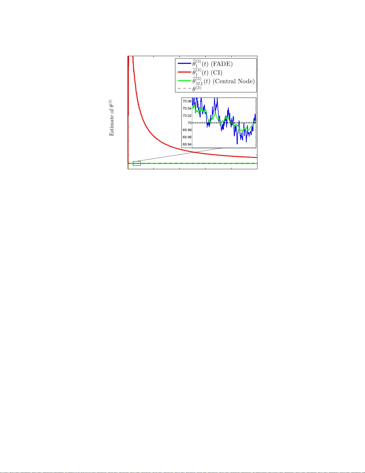
1 F ADE: F ast and Asymptotical ly ef fici ent Distrib ute d Es timator f or dynamic netw orks Ant ´ onio Sim ˜ oes and Jo ˜ a o Xavier , Member , IEEE Abstract Consider a set of agents t hat wish to estimate a vector of parameters of their mutual interest. For this estimation goal, agents can sense and c ommunicate. When sensing, an ag ent measures (in additi ve gaussian no ise) linear combinations of the unkno wn vector of parameters. W hen communicating, an agent can broadcast information to a few other agents, by using the channels that happen t o be randomly at its disposal at the ti me. T o coordinate t he agents t owards their esti mation goal, we propose a novel algorithm called F ADE (Fast and Asymptotically efficient Distributed Estimator), in which agents collaborate at discrete time-steps; at each time-step, agents sense and commun icate just once, while also updating their o wn estimate of the u nkno wn vector of parameters. F ADE enjoys fiv e attractive features: fir st, it is an intuitive estimator , simple to deriv e; second, i t withstands dynamic networks, that is, networks whose communication channels change randomly over time; third, it is strongly consistent in that, as time-steps play out, each agent’ s local estimate con verg es (almost surely) to the tr ue vector of parameters; fourth, it is both asymptotically unbiased and efficient, which means that, across time, each agent’ s estimate becomes unbiased and the mean-square error (MSE) of each agent’ s estimate vanish es to zero at the same rate of the MSE of the optimal estimator at an almighty central node; fifth, and most importantly , when compared with a state-of-art consensus+ innovation (CI) algorithm, it yields estimates with outstandingly lower mean-square errors, for the same number of communications—for example, in a sparsely con nected network model with 50 agents, we fi nd t hrough numerical simulations that the reduction can be dramatic, reaching sev eral orders of magnitude. Index T erms Distributed estimation, linear-gaussian models, dynamic networks, consensus+in nov ations I . I N T R O D U C T I O N D A T A is increa sin gly collected by spatially distributed agents, the term agent meaning some p hysical d evice that measure s d ata locally , say , a ro b ot. Moreover , not on ly is the data at th ese agen ts being collected with at an ever-gro wing rate and precision ( as former ly pricy high -quality sensor s such as h igh-resolu tio n cameras have meanwhile b ecame affordab le c o mmodities), but the numb er of ag ents the m selves collecting the data is soaring . Indeed , a present-day w ir eless sensor ne twork f or agr iculture precision easily sp ans tenths, if not hundr eds, o f agents, not to mention th e bloomin g vehicular networks or m obile internet-o f-things whose size will escalate to This work was supported in part by the Fundac ¸ ˜ ao para a Ci ˆ encia e T ecnol ogia, Portugal, under Project UID/EEA/50009/2013 and Grant PD/BD/13501 3/2017. (Correspond ing author: Ant ´ onio Sim ˜ oes.) The authors are with the Instituto Superior T ´ ecni co, Univ ersidad e de Lisboa, 1649-004 Lisbon, Portugal, and also with the Institute for Systems and Robotics, Laboratory for Robotics and Enginee ring Systems, 1049-001 Lisbon, Portugal. (e-mail: asimoes@isr.ist.ut l.pt; jxavier@ isr.ist.utl.pt) . ev en larger scales [ 1]. Th is steadily incr ease in bo th the volume of data an d the number o f its co llectors, howe ver , is at odds with the usua l way of extractin g in formation f rom data in distributed setup s: c e ntralized p rocessing. Centralized processing. In centralized p r ocessing, the data co llec te d by the a gents is u sually first rou ted in raw form (o r maybe slightly digested ) to a special central agent th a t then per forms the bulk of the nee ded comp u tations on the in c o ming data to squeeze out the desired in formation . Centralized p r ocessing is poo r ly suited to the current trend o f big data in distributed m ulti-agent systems, for centralized p rocessing is too fragile an d cum b ersome. Fragile bec a use, as soon as the central agen t breaks down, th e whole infr a structure o f agents is ren dered pointless, incapable of reasoning fro m the po uring data; cumb ersome because, as d ata falls on the agents at increasin g speeds and volumes, the capacity of the ph ysical p athways that convey the data to the central ag ent must swell in tandem until, of course, this cap acity hits a f u ndamen ta l limit (such as bandw id th o f av ailable wir eless chann els) and the show stops. This explains why ce n tralized processing is gradually eclipsing, g iving way to g r owing research o n a different appr oach for pro cessing data th at mesh es better with c urrent trend s: distributed pr ocessing. Distribu ted processing. The vision of d istributed processing is to u ntether the data-c ollecting agen ts from the central agent and to have the data- collecting agen ts recrea te them selves the centralized solutio n, by pr operly coo rdinating the agen ts in the fo rm of short m essages exchan ged locally between them . Thus, no central agent exists and no particular agent is key; all equally share the computatio n burden. As a result, distributed processing is more robust. If an agent brea ks down, the who le infrastructure does not come to a halt: just the particular data stream o f the faulty ag ent ceases to in form th e solution, with the rem a in ing agents keeping to collaborate to reason f rom their co llec ti ve data. In sum, sud den catastroph e in centra lized processing (as happen ing when the central agen t collap ses) gives place to gr aceful degrad ation in distributed p r ocessing. Distributed pro cessing also do es away with the p roblem of needing larger and larger capac ities for the physical pathways that relay the voluminou s collec ted data to th e central agent, f or the simple reason th at the central ag ent is crossed out from the picture. Not that a ny f orm of com munication fr om agents beco mes un necessary; agents do need to commu nicate to c o ordinate. But distributed pro cessing aims at h aving the agen ts to exchan ge short messages only , each message ideally abo ut the size of the info rmation that is d esired to squee z e out of the d a ta—a goal which requ ires modest capacities f o r th e co m munication ch annels. Closest related work on distributed estimation. Research on distributed pro cessing develops vigorou sly along se veral exciting threa d s, among them distributed optimization , filter in g, detection, and estima tio n. The literature is too vast to d iscu ss at len gth here, so we point the reader to referen ces [2]–[ 14], a c ross-section of representative work. This paper contributes to th e th read o f d istributed estimation. T o put o u r work in perspective, we n ow single out from this thread som e of th e closest r esearch. Most o f such research assumes a com mon backd rop: a set o f agents is linked by a communica tio n network, with the ag ents co llecting local data about the same vector of parameters; the challen ge is to create an algorithm th a t coord in ates the agents b y specify ing what they sh o uld commu nicate to each other alo ng time over th e available commun ication channels so th a t the agents arrive at a n estimate o f th e vector of par ameters, preferab ly an estimate as goo d as a cen tral no de would p rovide for the same time horizon. Against this shared backdro p, details vary . For example, [ 15] con siders a lin ear-gaussian measur ement model at each agent, the measur e ment matrices being time-variant and the ob servation noise p ossibly c orrelated a c ross 2 agents, though the commu nication n etwork is assumed static, n o t dynam ic (so, c o mmunicatio n chann els d o n ot change alo ng time) . For this setup, the author s work out a d istributed estimator , for which they are able to secu re a much desired feature: they p r ove that the prop osed estimator is efficient , in that its mean-squa re error (MSE) decays at the same rate o f the MSE of the centralized estima to r , as tim es unfold s. Scenarios in wh ich the vecto r of parameters cha n ges over time, po ssibly over dyn amic network s, can b e tackled by the successful suite of distributed algor ithms of th e diffusion type, developed, fo r instance, in [9], [1 0], [1 6], [17]. Being a b le to tr a ck time-varying para m eters, this type of algor ithms is fitted to distributed least-mean squares (LMS) or Kalman filtering ap plications, applica tio ns in wh ic h these diffusion algorithm s can , in fact, be p roved to be stable in the mean -square sen se. W e believe that the work that most resembles o u rs, howe ver , is th e accomplishe d consensus+innovatio n s (CI) algorithm , p ut f o rward in [ 7]. In deed, similar to what we assume in this p aper, the autho rs of [ 7] consider a static vector of p arameters, measured at each agen t throu gh a no ise-additive linear model, and a dyn amic commu nication network link in g the agents that chang e s random ly over time. Th us, altho ugh the CI algor ithm is applicab le to a broade r range o f scen arios (e.g., g aussian no ise is not assumed in [7]), we will use it as a benchmar k thr ougho u t the paper, both in section III, where we contrast its f orm with ou r F ADE algorithm , and in section V, where we compare their performan ce in practice. (Other distributed algo r ithms built ar ound the consensus+inn ov ations princ ip le, and not necessarily for estimation pu rposes, can b e found in [6]–[8], [18], [19].) Contributions. W e con tribute a distributed estimator called F ADE (Fast and Asymp totically e fficient Distributed Estimator), which coordina tes agents m easuring a comm o n vector o f parameter s in a linear-gaussian model and commun icating with each oth e r over a set of chan nels that change s random ly over time. F ADE is endowed with se veral assets, both on the th e o retical side an d o n th e pr actical side. On the theo retical side, F ADE is simple to der i ve, emerging from th e cen tral estimator after a couple of in tuiti ve steps. (By compar ison, the blueprint of the CI algor ithm [7], say , is somehow more inv olved to a r riv e at, resorting to the machiner y o f stochastic app roximation with mixed time- scales—perhaps a comp lexity price to pay for its more general applicability . ) More importan tly , F ADE comes with stron g convergence guar antees: it is strongly conv ergent (estimates conv erge to th e true parameter s with p robability one); it is asy mptotically unbiased (bias of th e estimates vanishes with time); and it is asy m ptotically efficient ( MSE of the estimates goes to zero at the same rate of the MSE of th e centr alized estimator, as time proce e d s). Ou r the o retical p roofs use tools from m artingale p robability theory . On the prac tica l side, F ADE is shown, throu gh numer ical simu latio ns, to sup ply estimates to the agents th at are notably more a c curate than the on es yielde d by the CI algo r ithm, for the same time period. Said in othe r words: although both F ADE an d the CI alg orithm are asymptotically efficient, numerical simulations show that F ADE reaches the asymptotic optimal perf ormance significan tly sooner . As an illustration, in on e of the simulations we find that the MSE of F ADE is lower than the MSE o f CI b y five ord ers of m a gnitude. Paper organization. W e organize th is paper as follows. In section II, we detail the m easurement and commun ica tion models, along with usual blanket assumptions, thus stating precisely the problem at hand. The problem is tackled in section II I, in which we derive our solution—th e F ADE algor ithm—whose strong theo retical convergence proper ties are laid ou t in sectio n IV. In section V, we co mpare by numer ical simulatio n the accuracy of F ADE with the accuracy o f the CI algorithm, bo th in a dense and a sp arse n etwork model. Sectio n VI closes the p a p er , with p a rting 3 conclusion s. Append ices give the proofs of theorem s stated thr ougho ut the p aper . I I . P RO B L E M S TA T E M E N T The vector of parameters th at the N a g ents wish to estimate is θ ∈ R d . The measurement model: how a gents measure θ . Each agent measures a linear map o f θ in ad ditiv e g aussian noise. Specifically , at tim e - step t = 1 , 2 , . . . , agent n measu res y n ( t ) = H n θ + v n ( t ) , (1) where H n ∈ R d n × d is the lin e ar map of ag e n t n , and v n ( t ) is g aussian noise, detailed in the following assumption. Assumption 1. ( Gaussian noise) For each ag ent n and time-step t , the ran dom variable v n ( t ) is a sample of a gaussian distribution with zero m ean and unit covariance, wr itten v n ( t ) ∼ N (0 , I d n ) . These ran dom variables are indepen d ent across agents and time; that is, v n ( t ) is in depende n t of v m ( s ) if n 6 = m or t 6 = s . As an aside, note that if the covariance o f the no ise was other than the iden tity matrix, say , Σ n 6 = I d n , then the unit-covariance feature could be restored at on c e by p remultiplyin g y n ( t ) with Σ − 1 / 2 n (redefinin g H n also in the process). In sum, this co n venient assumption entails no loss of gen erality . W e also need a basic observability assumption th at states θ can be iden tified from all the agen ts’ measure- ments. Specifically , stack the o b servations ( 1) in th e column vector y ( t ) =  y 1 ( t ) T , y 2 ( t ) T , . . . , y N ( t ) T  T ∈ R d 1 + d 2 + ··· + d N ; this gives y ( t ) = H θ + v ( t ) , whe re H = h H T 1 H T 2 · · · H T N i T ∈ R ( d 1 + d 2 + ··· + d N ) × d and v ( t ) =  v 1 ( t ) T , v 2 ( t ) T , . . . , v N ( t ) T  T . The vector y ( t ) can be seen as a n etwork-wide measureme n t: it collects the measuremen ts at time t from all the agents. W e assume that θ is identifiab le f rom these network - wide me a surements, which is equiv alent to assuming that the network- wide sen sing m atrix H is f ull column -rank. Assumption 2. ( Global observability) The matrix H is full co lumn-ran k. For the scalar case d = d 1 = d 2 = · · · =1 , this assumption just means that some sensing gain H n ∈ R is nonzero. In gen eral, note that this assump tion exempts the local sensing matrices H 1 , . . . , H n from any p articular stru cture; e.g., all sensing matr ice s co uld ev en lack fu ll column- rank, wh ich would make θ un indentifiable from any agent (if H n is not full column-ran k, then ag ent n can no t discern between θ from θ + δ , wh ere δ is any non z ero vector in the kernel of H n ). Assumptio n 2 en sures tha t θ can b e iden tified wh enever agen ts work as a team . The communication model: how ag ents can exchange information. The co mmunication network lin king the agents is mod elled as an un directed g raph th at cha n ges r andomly over time : at tim e-step t , we call this grap h G ( t ) = ( V , E ( t )) . (2) Here, V = { 1 , 2 , . . . , N } is the set of N agents, and E ( t ) is the set of edges available at time step t . An edge between agen ts n an d m models a communication chann e l between them; note that, b ecause the graph is undirected, the ch annels are b idirectional (whic h means that if, at a g iven time step t , agent n can send info rmation to agent m , then the reverse also holds: ag ent m can send in formation to agent n as well). W e let channels ap pear an d disappe a r rando mly over time, to model agents that move arou nd or data packets that get lost; theref o re, the terms of the sequ e n ce of ed g e-sets E (1) , E (2) , E (3 ) , . . . from (2) vary alo n g time. Note , howe ver , that each ter m in this sequen ce necessarily takes values in a finite collectio n of e d ge-sets, say , a collection 4 with K edge- sets: E ( t ) ∈ {E 1 , . . . , E K } . Su ch collection is finite bec a u se each E ( t ) must be an edge- set over the node-set V and, since V is fixed, the collection of all edg e-sets on V is itself finite. Of course, for a particu lar application scenario, no t all possible ed ge-sets need to tu r n out: in fact, the co llection {E 1 , . . . , E K } is the subset of those edg e-sets that have a strictly p ositiv e pro bability o f tu r ning o ut fo r th is a pplication scenario. Finally , we assume that the sequence E (1) , E (2) , E (3 ) , . . . satisfies a standa r d a n d b asic prope r ty called average connectivity . Assumption 3. (A verage connectivity) The ran dom sequence of ed ge-sets E (1) , E (2) , E (3) , . . . , is indep endent and ide ntically distributed (i.i.d.). Each edge-set E ( t ) takes values in th e finite collection {E 1 , . . . , E K } with probab ility π k = P ( E ( t ) = E k ) , whe r e π k > 0 an d P K k =1 π k = 1 . Moreover, the average edge-set is con n ected, that is, the grap h  V , S K k =1 E K  is connected . Recall that a g raph is conn ected if th ere is a path b etween any two nod es, the path c o nsisting po ssibly of many edges. Assumption 3 mea ns that the average co mmunicatio n graph is co nnected. In other words, the a ssum ption means that if w e overlay all ed ge-sets with p ositi ve p robability of o ccurring , a connec ted gra p h results. Of cour se, at each time step t the graph G ( t ) = ( V , E ( t )) is a llowed to b e disconne c ted; such is the case, fo r instance, in single-neigh bor gossip-like proto cols where only two neig hbour agents talk at a time (in such a case, each E ( t ) contains only one edge) . The problem addressed in this pa per . W e add r ess th e pr o blem of crea ting an algorithm that runs at each a gent and th at, by using the locally av ailable sensing and commun ication resources, provid es an estimate—as accura te as possible—of θ at eac h agent. For this pr oblem we propose F ADE, a Fast an d Asy m ptotically efficient Distributed Estimator, which we deriv e in th e next section. I I I . D E R I V I N G FA D E F ADE is an intuitive algorith m, simple to derive. For clarity , we first fo cus in section III-A on a scalar p arameter, θ ∈ R ; the extension to the vector case, θ ∈ R d , is plain an d ap pears in section II I-B. A. F ADE algorithm fo r scalar parameter W e d eriv e F ADE in a p rogression of three easy steps, starting fro m th e stance of an alm ig hty central node . Step 1. The optimal alg orithm at a central node. W e start by d eriving the optimal estimator . This is the estimator that could r u n only at a cen tral node—a fictitious, almig hty node that would know instantan e o usly the m easurements of all the ag ents. Such optimal estimator is the minimum variance and un biased (MVU) estimator or, in our linear-gaussian setup, also th e maximum likeliho od (ML ) estimator . It is g i ven by a weighted comb ination of the average measureme nts of the agen ts; specifically , at time t = 1 , 2 , 3 , . . . , it is given by b θ ( t ) = N X m =1 1 N c m y m ( t ) , (3) where c m =  (1 / N ) P N i =1 h 2 i  − 1 h m is the weight of agent m , an d y m ( t ) = 1 t t X s =1 y m ( s ) (4) 5 is the average measuremen t of agent m by time t . W e skip the details on how to obtain the optimal estimator (3) because they are well-known (e.g. , see [20]). Now , we ca n wr ite (4) in the recursive f orm y m ( t ) = y m ( t − 1) + (1 /t )( y m ( t ) − y m ( t − 1)) ; and plugg ing this recursion in (3) gives the following up date for th e optimal estimator : b θ ( t ) = 1 N N X m =1  b θ ( t − 1) + 1 t c m ( y m ( t ) − y m ( t − 1))  , (5) for t = 1 , 2 , 3 , . . . , where we set b θ (0) = 0 an d y m (0) = 0 for all m . Update (5) reveals an interesting feature: at time step t , the op timal estimato r in (5) needs only to know fr om each agen t m the number c m ( y m ( t ) − y m ( t − 1)) . This means that, b esides a central no d e, th e optimal estima to r can also run in a c ertain distributed scenar io —-a scenar io in which the co mmunication gr aph is static and complete, as we show in th e next step. Step 2. The optima l algorithm in a sta tic, complete graph Consider a static, com plete grap h. Being static, its edges are fixed over time. Being com plete, it contains all possible edges, that is, any pair of agents is lin ked by an edge. I n th is g raph a ny given ag ent n can ob tain whatever inform ation it needs from any oth er agent m at any time step; agen t m has on ly to send th a t informa tio n thr ough the chan nel link ing agents n a n d m . In p articular, agent m can send c m ( y m ( t ) − y m ( t − 1)) . So , any agen t n ca n ca r ry out the optimal upd a te (5). Letting, then, b θ n ( t ) be the estimate at ag ent n in such a graph, we hav e b θ n ( t )= 1 N N X m =1  b θ n ( t − 1)+ 1 t c m ( y m ( t ) − y m ( t − 1))  , (6) with b θ n (0) = 0 . Note that the agents’ estimates keep the same throu gh time, b θ 1 ( t ) = b θ 2 ( t ) = · · · = b θ N ( t ) , and recreate the optimal upd ate in (5). Let us pass to a mor e conv enient vector form. Stack all agent’ s estimates in the vector b θ ( t ) =  b θ 1 ( t ) , . . . , b θ N ( t )  ∈ R N . I t follows from (6) th at b θ ( t ) = J  b θ ( t − 1) + 1 t C ( y ( t ) − y ( t ))  , (7) where J = 11 T / N (with 1 = (1 , 1 , . . . , 1) ∈ R N ) is the con sensus matrix , C ∈ R N × N is a diag onal matr ix with n th diagonal entry equ a l to c n , y ( t ) = ( y 1 ( t ) , . . . , y N ( t )) ∈ R N , and y ( t ) = ( y 1 ( t ) , . . . , y N ( t )) ∈ R N . Step 3. The F ADE algorit hm in a genera l graph. The optimal estimator (7) is unab le to run in a gen eral grap h changin g over tim e. In deed, let E ( t ) be the set o f a vailable edg es for commu nication at time step t . A t this time step, o nly a few commu nication channels typ ically link a given agent n to other agen ts. Specifically , agent n can receive inform ation only from tho se ag ents m for which the (un directed) ed ge { n, m } is in E ( t ) , a subset called the neighbo rhood of age n t n at time step t and den oted by N n ( t ) = { m 6 = n : { n, m } ∈ E ( t ) } . Sadly , the update (7) requires agent n to rec e i ve info rmation, not just from some neighbo r ag ents, but from a ll ag ents. As such, the update (7) canno t run in a g eneral g raph. Inspired by the form o f the rec ursion (7), howev er, we now suggest a simp le modifica tio n that can run in gen eral graphs. The key id ea is to no te that the obstruction is ju st th e consensus matrix J . In deed, each entry ( n, m ) of J is non-zero (to be more specific, J nm = 1 / N ): this makes th e up date at agent n to dep e n d on the info rmation 6 at any o ther agen t m . But, would that entry be zer o , and the upd ate at ag ent n would no longer depend o n th e informa tio n at agent m . Our idea n ow almost sugg ests itself: simply replace th e consensu s matr ix J in (7) with a m atrix, say W ( t ) , tha t has the rig ht spar sity at time t . T h at is, a m atrix W ( t ) where each entry W nm ( t ) non zero if and o nly if ag ents n and m are neig hbors at time t : W nm ( t ) 6 = 0 if and only if { n, m } ∈ E ( t ) . W e finally arrive at o u r F ADE algorithm: b θ ( t ) = W ( t )  b θ ( t − 1) + 1 t C ( y ( t ) − y ( t − 1))  , (8) or , expressed fo r a generic age n t n : b θ n ( t )= N X m =1 W nm ( t )  b θ m ( t − 1)+ 1 t c m ( y m ( t ) − y m ( t − 1))  . (9) About pr o perties on the matr ices W ( t ) that m ake F ADE su c ceed, we will say much more in the next section III-C. T o c o nclude, we interpr et each itera tion of F ADE (9) in terms of sensing an d commu nication. The iteratio n ( 9) can be seen as unfoldin g in two halves: in the first half, each a g ent m = 1 , . . . , N updates its estimate by absorbing its m easurement, θ m ( t ) = b θ m ( t − 1 ) + 1 t c m ( y m ( t ) − y m ( t − 1)) , thus using its sensing r e so urce; in the seco nd h alf, e a ch ag ent m = 1 , . . . , N send s its upd ates θ m ( t ) to its neigh b ors, thus using is co m munication resource. Upon receiving the upd ates θ m ( t ) from its neighb ors, each agen t n com bines these up dates with its own, b θ n ( t ) = P N m =1 W nm ( t ) θ m ( t ) . Comparing the F AD E algorithm wit h the CI alg orithm. W e now compare the form of the F ADE algor ith m in (8) with the consensu s+innovations (CI) algorith m from [7], h olding in mind the optimal estimator in (7) as a refer ence point. W e will see that, in a certain sense, F ADE is clo ser to the idealized estimator ( 7). Let e θ m ( t ) be the estimate of the parameter θ that the CI algorithm prod u ces at agen t m and at tim e t ; letting e θ ( t ) =  e θ 1 ( t ) , . . . , e θ N ( t )  ∈ R N be the vector o f estimates across the network, we have ( see [7]) e θ ( t )= ( I N − β ( t ) L ( t )) e θ ( t − 1)+ α ( t ) C  y ( t ) −H e θ ( t − 1)  . (10) Here, L ( t ) is the lap la c ian matrix of the graph G ( t ) = ( V , E ( t )) , that is, a N × N matrix filled w ith zeros save for th e no ndiagon al entr ies correp o nding to ed g es in E ( t ) (wh ich are filled with − 1 ) and th e diago n al entries (which are filled with the n umber of neig hbors of the co rrespond ing agen t, thus mak ing L ( t ) 1 = 0 ); the ma tr ix H ∈ R N × N is diag onal with n th diagon al entry equal to h n , an d both α ( t ) and β ( t ) ar e positive step sizes which obey certain requir ements: for our purposes, α ( t ) = 1 / t and β ( t ) = 1 / t r with 0 < r < 1 / 2 do. Now , letting W ( t ) = I N − β ( t ) L ( t ) and α ( t ) = 1 /t , we ca n rewrite (10) as e θ ( t ) = W ( t ) e θ ( t − 1 ) + 1 t C  y ( t ) − H e θ ( t − 1)  . (11) When we compare b oth the F ADE (8) an d the CI (11) updates with the ideal update (7), two main differences spring up: fir st, even if the comm unication grap h was static and fully connected (so , with laplacian matrix L = N I N − 11 T ), the CI algo rithm would d iffer fro m the optimal form ( 7), wher eas the F ADE up date and the o ptimal on e would become the same (for we could assign W ( t ) = J ); secon d , the rightmost term in the optimal r ecursion ( 7)—that is, the in novation term y ( t ) − y ( t − 1 ) —finds itself replaced by y ( t ) − H e θ ( t − 1) in the CI algor ithm, whereas it is left intact in F ADE. So, the alg orithm most faithful to the idealized estimator ( 7) is F ADE. Th is gives us an inkling o f why F ADE estimates θ with an accura cy closer to th e accur acy of a ce n tral nod e outstanding ly soo ner than the CI algo rithm, as th e n u merical simu la tio ns in section V attest. 7 B. F ADE algorithm fo r a vector of pa rameter s Extendin g the F ADE algor ithm (8) to a vector o f parame ters θ ∈ R d with d > 1 is plain. Recall the F ADE update for a scalar p a rameter, at each agent n g i ven in ( 9). In the case o f a vector of p arameters, the scalar h i ∈ R become s a matrix H i ∈ R d i × d : rec a ll (1). A c cordingly , we can upgr ade the scalar c m ∈ R to the matrix C m = (1 / N ) N X i =1 H T i H i ! − 1 H T m ∈ R d × d m (12) and the F ADE update to b θ n ( t ) = N X m =1 W nm ( t )  b θ m ( t − 1)+ 1 t C m ( y m ( t ) − y m ( t − 1))  , (13) where b θ m ( t ) ∈ R d . This is the g eneral F ADE alg orithm at each agent n ; or, repacked in matrix form, b θ ( t ) = ( W ( t ) ⊗ I d )  b θ ( t − 1) + 1 t C ( y ( t ) − y ( t − 1))  , (14) where b θ ( t ) =  b θ 1 ( t ) T , . . . , b θ N ( t ) T  T ∈ R dN , ⊗ is Kron ecker pr oduct, C ∈ R dN × ( d 1 + d 2 + ··· + d N ) is a b lock- diagona l m atrix with n th block equ al to C n , y ( t ) =  y 1 ( t ) T , . . . , y N ( t ) T  T ∈ R d 1 + ··· + d N , and y ( t ) =  y 1 ( t ) T , . . . , y N ( t ) T  T ∈ R d 1 + ··· + d N . C. The weigh t matrices W ( t ) W e n ow give cond itions on the weight m atrices W ( t ) that allow F ADE to succeed . First, recall that each W ( t ) mir rors the sparsity of the edge-set E ( t ) . That is, en try W mn ( t ) is n onzero if and only if there is an ed g e b etween agents n and m in the e d ge-set E ( t ) . W e assume that ea ch W ( t ) is symmetr ic  W ( t ) = W ( t ) T  ; ha s non negativ e entries ( W nm ( t ) ≥ 0 ); and is row- stochastic, i.e., the entr ies in each of its rows sum to o ne ( W ( t ) 1 = 1 ). W e also assume that e a ch diagon a l en tr y of W ( t ) is po siti ve: W nn ( t ) > 0 for all n . No te that the con sensus m atrix J (which W ( t ) is m eant to r eplace in (7)) has all these prop erties. Metropolis weights. A simple way to make sure these prop erties hold for each matrix W ( t ) is to ch oose the en tries of W ( t ) a s in the Metropo lis rule [21]: W nm ( t ) = 1 / ( max { d n ( t ) , d m ( t ) } + 1 ) , if ag ents n and m ar e neig hbors in E ( t ) ; W nm ( t ) = 1 − P m ∈N n ( t ) W nm ( t ) , if n = m ; and W nm ( t ) = 0 , otherwise. He re, N n ( t ) = { m : { n, m } ∈ E ( t ) } is the neig hborh o od o f a g ent n (in the gr aph G ( t ) = ( V , E ( t )) , and d n ( t ) is the degree of agent n , i.e., the num ber of its ne ig hbors (the cardina lity of the set N n ( t ) ). The Metropolis rule allows eac h agent n to compute its weig hts ( W nm ( t ) for m = 1 , . . . , N ) locally: agent n ignores th e g lobal edge-set E ( t ) , a fit proper ty in practice, for otherwise agent n would need to know wh ich chan n els tu rned out in far away corners of the network at ea ch time step t ; in the Metropo lis tu le, a g ent n ne eds to kn ow o n ly its degree and the d egrees of its neigh b ors (an easy-to-g et informa tio n that can be passed b y th e ne ig hbors th emselves). 8 The Metropo lis rule, then , associates to e a ch edge- set E ( t ) a weig ht ma trix W ( t ) . Because the edge-set E ( t ) is random and takes values in a finite collectio n of edge-sets {E 1 , . . . , E K } with proba b ility π k = P ( E ( t ) = E k ) , it follows likewise that W ( t ) is rando m an d takes values in a finite collection of weigh ting matrices, say , { W 1 , . . . , W K } , w ith corr esponding prob ability π k = P ( W ( t ) = W k ) . Note also that, as a consequence , the sequence W ( t ) , t = 1 , 2 , . . . , is i.i.d. In su m, we hav e the f ollowing assumption on the weigh t matr ices. Assumption 4. ( W eight matrices) Each weig ht m atrix W ( t ) in (14) mirrors the spar sity of the edge- set E ( t ) . Also, e a ch W ( t ) has a positiv e diag onal and is symme tric, non negati ve, and r ow-stochastic. Mor eover , each W ( t ) takes values in a finite set { W 1 , . . . , W K } with pr obability π k = P ( W ( t ) = W k ) (whe re π k = P ( E ( t ) = E k ) ), and the sequence W ( t ) , t = 1 , 2 , . . . is i.i.d. . This assum ption, togethe r with assumption 3 on a vera g e co nnectivity of the ed ge-sets E ( t ) , guaran tees key proper ties for two matrice s that will prove impo rtant in the theo retical ana ly sis o f F ADE (see next section IV): the average weighting matrix W = E ( W ( t )) = P K k =1 π k W k and the average off-consensus m atrix f W = E  f W ( t ) T f W ( t )  = K X k =1 π k f W T k f W k , (15) with f W ( t ) = ( I N − J ) W ( t )( I N − J ) (16) and f W k = ( I N − J ) W k ( I N − J ) . The key p roperties ar e stated in the following lemma . Lemma 1: Let assumptio n s 3 and 4 hold. Th en, W is a primitiv e matr ix an d f W is a co ntraction matrix. Recall that a prim itive matr ix is a square nonn egati ve m atrix A such that, fo r some p ositi ve in teger m , th e matrix A m is positive (i.e. , each entry o f A m is a positive nu m ber). In our case, note that W is a symmetric matrix, wh ich makes all of its eigenv alues real-valued; moreover, becau se W 1 = 1 , one of th ese eigen values is the num ber 1 w ith the vector 1 as its associated eig en vector . Now , giv en that W is a no nnegative matrix and th at lemma 1 states W is also a primitive matrix, it follows fr om standard Perron -Frobeniu s theory (see [2 2]) th at 1 is, in fact, th e domin ant eigenv alue: if λ 6 = 1 is anoth er eig en value o f W , th en | λ | < 1 . Finally , the matrix f W being a contra c tio n means that its spectral radiu s is strictly less than one, ρ  f W  < 1 . The pr oof o f lemma 1 is om itted becau se these these gen eral p roperties are well-known and f ollow fr om classic Perron-Fr obenius th eory: fo r examp le, [2 3] sh ows that W is a pr imitiv e matrix in Pr oposition 1 .4, and that f W is a contrac tio n matrix in p. 35 . I V . T H E O R E T I C A L A NA L Y S I S O F FA D E In this section, we state the two chief proper ties th at F ADE enjoys: almost sure co n vergence to th e true vector of parameter s, and asympto tic un biasedness and efficiency . W e start by e stab lishing almost su re (a.s.) con vergence. Let b θ n (1) , b θ n (2) , b θ n (3) , . . . , be the sequence of estimates of the vector of p arameters θ th at F ADE pro duces at agen t n : see (13). No te that this sequen c e is rando m becau se both th e measurem ents an d the edges are random. Theor em 1 states that the sequence converges alm o st surely to the corr ect vector of parameters θ . Theorem 1 (F ADE conver ges a lmost surely): Let assump tions 1, 2, 3, and 4 hold. Th en, lim t →∞ b θ n ( t ) = θ , a.s., for n = 1 , 2 , . . . , N . 9 Pr o o f: See appen dix A. W e now pass to asymptotic un biasedness and efficiency . Asymptotic un biasedness means that the seq uence of estimates b θ n (1) , b θ n (2) , b θ n (3) , . . . , b ecomes u nbiased, th at is, E  b θ n ( t )  conv erges to θ , as t → ∞ . Asymptotic efficiency means that the mean-square error (MSE) of ea c h term in the seque nce of estima tes decays at the same rate as th e o ptimal estimator . Specifically , let b θ ML ( t ) be the optimal (maximum- likelihood) estimator—the estimator that run s at a ce n tral nod e—, g i ven by b θ ML ( t ) = N X n =1 1 N C n y n ( t ) , (17) where C n is d efined in (12) and y n ( t ) in (4). (For a scalar param e ter , θ ∈ R , this estimator coinc ides with the one gi ven in (3).) W ith standard tools [20], it is easy to show that th e optimal e stimator is u nbiased at all times, E  b θ ML ( t )  = θ , an d its MSE, g i ven by MSE  b θ ML ( t )  = E     b θ ML ( t ) − θ    2  , decays to zero as fo llows: MSE  b θ ML ( t )  = tr   P N n =1 H T n H n  − 1  t . (18) Asymptotic efficiency of F ADE means that the decay rate of the MSE of the F ADE estimate b θ m ( t ) at any agen t matches the decay rate of MSE o f the optimal estimator at the central node. The result is stated precisely in the next the o rem. Theorem 2 (F ADE is asympto tically unb iased a nd efficient): Let assumptions 1, 2, 3, and 4 h old. Then, lim t →∞ E  b θ n ( t )  = θ, an d lim t →∞ MSE  b θ n ( t )  MSE  b θ ML ( t )  = 1 , (19) for n = 1 , 2 , . . . , N . Pr o o f: See appen dix B. In this sense, F ADE succee d s in makin g all ag ents as powerful as the central node. V . N U M E R I C A L S I M U L AT I O N S W e co mpare th ree estimato rs: the p roposed F ADE estimator b θ ( t ) (given in (14)), the state-of-ar t CI estimator e θ ( t ) from [7] (given in (10) for scalar p arameters), and th e centralized estima to r b θ ML ( t ) (given in (17)). W e compare the estimators in two k inds of simulation s. I n the first kind of simu lations, section V - A, we look at alm o st sure conver gence (theor em 1); we c o mpare the speed at which the estimato rs conver ge to th e true vecto r of parameter s θ . I n the second kind of simulatio ns, section V -B , we look at MSEs (theor em 2); we compar e the speed at which the ac curacy of all estimator s, as me a su red by the ir MSEs, goes to zero. Simulation setup. T o com pare the estimato rs, we set up a dense network an d a spar se one. Both networks consist of a set V of N = 50 agen ts. Also, both ne tworks h av e their e dges changing rand omly over time. For the dense network , the rando m ed ge- set E ( t ) takes values in a finite collectio n of K = 15 edge- sets, {E 1 , E 2 , . . . , E K } , with th is collection satisfying assumption 3 ; that is, the gr a p h G =  V , S K k =1 E k  , which r esults f rom overlaying all edg e - sets in the collection {E 1 , E 2 , . . . , E K } , is c onnected. W e call th is network dense beca u se G is den se. Spec ifically , a bout 79 % pairs 10 of agen ts have an edge between them in the edge - set ∪ K k =1 E k and, for e ach E k , the a verage d egree (n u mber o f neighbo rs) o f an agent is abou t six. As for the sparse network , the correspo nding grap h G con nects directly just 28% pairs of agen ts, and th e average d egree of the agents p er E k drops to a num ber close to on e . Whether the network is den se or sparse, agent n measures the vector of par ameters θ = (100 , 1 20 , 70 , 9 0 , 200) ∈ R 5 throug h th e same linear-gaussian sensing m odel y n ( t ) = H n θ + v n ( t ) , where v n ( t ) is standard gaussian noise and H n ∈ R 8 × 5 . W e made ea ch matrix H n to hav e only rank 4 ; this is to make sure that no single agent could identify θ , ev en if given an infinite supply of measurements. Thu s, the vector o f p a rameters θ is identifiable only throug h collabora tion (the set o f m atrices H n , n = 1 , . . . , N chosen secures g lobal o b servability , see assumption 2 ). Finally , we use the Metro p olis weig hts fo r F ADE (see section III-C), and the step- sizes α ( t ) = 1 /t and β ( t ) = 1 /t 0 . 05 for CI (see (1 0)). A. F irst kind of simula tions: almost su r e con ver gence All three estimators—F ADE b θ ( t ) , CI e θ ( t ) , and th e centralized o ne b θ ML ( t ) —con verge almost surely (a .s.) to θ as the num ber of commu nications grows un bound e d: lim t →∞ b θ n ( t ) = lim t →∞ e θ n ( t ) = lim t →∞ b θ ML ( t ) = θ , a.s., (20) for any a gent n . For the op timal estimator, ( 20) fo llows at once from ( 17) an d the strong law of large num bers (which assures lim t →∞ y n ( t ) = H n θ almost sur e ly); f or F ADE, see th e proof of theor em 1; fo r CI, see [7]. But the theoretical analysis fails to tell u s ho w fast the conver gence in (20) occurs. The reason is that the analysis is asy mptotic; it explains only wh at happen s in the long run, for t = ∞ . I n this remote h o rizon—after an infi nite number of co mmunication s—(20 ) shows that all estimators lo ok the same. W e igno re, howe ver , how the estimator s compare in a more realistic h orizon: after a numb er of com m unications that is p ractical . Results for the sparse network. W e u se th e challen ging sparse network to find the speeds at which the thr ee estimators appro ach the limit ( 20). Specifically , we fo c u s on agent 1 and track its e stimate of the third en try of the vector of p arameters θ = (100 , 120 , 70 , 90 , 200) , as y ie ld ed by the th ree estimators: b θ (3) 1 ( t ) for F ADE, e θ (3) 1 ( t ) f or CI, and b θ (3) ML ( t ) for the centr alized estimator . Accord in g to (20), all estimates go to θ (3) = 70 , lim t →∞ b θ (3) 1 ( t ) = lim t →∞ e θ (3) 1 ( t ) = lim t →∞ b θ (3) ML ( t ) = 70 , a.s.. (21) Figure 1 reveals, h owe ver, that the estimates go to θ (3) = 70 at stunn ingly different speeds: CI lags a p preciably behind, while F ADE goes hand in han d with th e swift c entralized estima to r . For th is example, we blin ded agent 1 to the third entry of θ , θ (3) , by filling the th ir d column o f the sensing matrix H 1 with zer os. Th is means that θ (3) has no bearing on the measurements o f ag e n t 1 , and th at θ (3) can only b e learned quic k ly a t agent 1 through effecti ve team work. Fig ure 1 shows that F ADE d eli vers such effective coordin ation, f or it supp lies agen t 1 with an acc u rate guess o f the missing par ameter , prom ptly . 11 0 1000 2000 3000 4000 5000 50 100 150 200 250 300 350 400 450 t E s t i m a t e o f ( 3 ) ( 3 ) 1 ( t ) ( F AD E ) ( 3 ) 1 ( t ) ( C I ) ( 3 ) M L ( t ) ( C e n t r a l No d e ) ( 3 ) Fig. 1: How the three estimates at agent 1 — b θ (3) 1 ( t ) for F ADE, e θ (3) 1 ( t ) for CI, and b θ (3) ML ( t ) for the centralized estimator—approac h their limit θ (3) = 70 in t he sparse netwo rk, along one path of 5000 time-steps. T he F ADE estimate i s on par wit h t he quick centralized estimate: the magnified box resolves t he time-steps between 250 and 500 . The CI estimate has a considerable relativ e error of about 20% , even after 5000 communications; in contrast, both F ADE and the centralized estimator attain a scant relativ e error of about 0 . 1% , as early as after 250 steps. B. Second kin d o f simulatio ns: sca led MS E s The MSEs o f the three e stima to rs decay to ze ro at the rate O (1 /t ) . Specifically , wh en we scale th e MSEs by the num ber of time-steps t , th e scaled MSEs conv erge to th e same limit: lim t →∞ t MSE  b θ n ( t )  = lim t →∞ t MSE  e θ n ( t )  = lim t →∞ t MSE  b θ ML ( t )  = tr   N X i =1 H T i H i ! − 1   , (22) for a ny ag ent n . For the optimal estimator, (22) follows fr o m (18); fo r F ADE, see the pro of of (19) in append ix B; for CI, see [7]. For the optimal e stima to r , the conver gence in (2 2) is instantaneou s. Th is is becau se t MSE  b θ ML ( t )  is con stant (so, already equ al to its limit fro m the first time-step); see (18). For F ADE and CI, howe ver , the available theor etical analysis is unab le to info rm abo ut h ow fast the conver gence in (22) takes place. As the following n u merical resu lts show , th e prop osed F ADE estimator conver ges o u tstandingly faster . Results for the dense network. W e look at the scaled MSEs that the three estimators (F ADE, CI, and the centralize d one) provide at ag e nt 1 for the dense n e twork model. W e run 1000 Mo nte-Carlos, each one co nsisting of a stretch of 12 5000 time-steps, and we a verage a t the en d the Monte-Carlos to find out how the scaled estimators— t MSE  b θ 1 ( t )  for F ADE, t MSE  e θ 1 ( t )  for CI, and t MSE  b θ ML ( t )  for the centralized estimator—behave throug hout th e time- steps t . Fig u re 2 shows the results: th e pro posed F ADE estimator follows clo sely the quick c entralized estimator , while the CI estimator is off by six o rders of magnitu de. Results for the sparse network. For th e sparse network , th e difference in perfo rmance grows e ven la rger, to sev en orders of magn itude; see Figure 3. V I . C O N C L U S I O N S W e proposed a new algo rithm for distrib uted parameter estimation with linear -gaussian measurements. Our algorithm , called F ADE (Fast and Asymptotically e fficient Distributed E stima to r), is simple to derive and copes with commun ication network s that ch a n ge r andomly . F ADE com e s with strong theoretical gu arantees: not o n ly is it stron gly con sistent, but also asymptotically efficient. Com p ared with a state-of-art con sensus+innovations algorithm , F ADE y ields estimates with significan tly smaller me a n-square- error (MSE)—in nume rical simulations, F ADE features estimates with MSEs that ca n b e six or seven order s of magnitu d e smaller . A P P E N D I X A P RO O F O F T H E O R E M 1 Scalar para meter . W e will p rove th e theo rem for the case o f a scalar param eter— θ ∈ R —f o r clar ity . The proo f for the gen eral vector case θ ∈ R d , d > 1 , is immediate an d le f t to the re a der . For the c a se of a scalar pa rameter, the n etwork-wide measurem ent vector y ( t ) = ( y 1 ( t ) , y 2 ( t ) , . . . , y N ( t )) T ∈ R N is y ( t ) = hθ + v ( t ) , w h ere h = ( h 1 , h 2 , . . . , h N ) T ∈ R N is a no nzero vector, tha n ks to assump tion 2. The F ADE algorith m is b θ ( t ) = W ( t )  b θ ( t − 1) + 1 t C ( y ( t ) − y ( t − 1))  , (23) for t ≥ 1 , with b θ (0 ) = 0 . Also, re c a ll that C is a diag onal matrix with n th-en try c n =  (1 / N ) P N i =1 h 2 i  − 1 h n , and y ( t ) = 1 t P t s =1 y ( s ) with y (0) = 0 . The goal is to show that lim t →∞ b θ ( t ) = θ 1 , a.s.. (24) The in-consensus and off-c onsensus ort hogonal decompo sition. Any vecto r u ∈ R N can be deco mposed a s an orthog onal sum of two vectors: one vector aligned with the vector 1 ∈ R N , and the o ther vector orth ogonal to 1 . That is, u = u ⊤ 1 + u ⊥ (25) where the scalar u ⊤ = 1 T u/ N ∈ R an d the vector u ⊥ = u − u ⊤ 1 . It follows that u ⊥ = ( I N − J ) v (recall th at J = 11 T / N ) is th e consensus m atrix. The vector u ⊤ 1 is called the in-con sensus comp o nent o f u ; the vector u ⊥ , its off-consensu s com ponent. Decompo sing as such the vector b θ ( t ) = b θ ⊤ ( t ) 1 + b θ ⊥ ( t ) , (26) 13 0 1000 2000 3000 4000 5000 0 1 2 3 4 5 6 7 x 10 7 t t × M SE ( • ( t )) e θ 1 ( t ) (C I) t × M S E ( b θ M L ( t )) (The ory) 0 1000 2000 3000 4000 5000 6.5 7 7.5 8 8.5 9 9.5 10 t t × M SE ( • ( t )) b θ 1 ( t ) (F AD E ) b θ M L ( t ) (C e nt r a l No de) t × M S E ( b θ M L ( t )) (The ory) Fig. 2: This fi gure compares throughout t i me, at agent 1 in the dense network, the scaled MSE of the optimal centralized estimator with the MSEs of two distributed estimators: the state-of-art CI estimator and the proposed F ADE estimator . The top plot sho ws the CI and centralized estimators; the bottom plot shows the F ADE and centralized estimators. The CI estimator is significantly outdistanced by the proposed F ADE estimator , with F ADE keeping up with the optimal centralized estimator: note that, f rom the top to the bottom plot, the range of the vertical axis shrinks by six orders of magnitude. we see that (2 4) amm ounts to lim t →∞ b θ ⊤ ( t ) = θ , a.s., (27 ) 14 0 1000 2000 3000 4000 5000 0 1 2 3 4 5 6 7 x 10 7 t t × M SE ( • ( t )) e θ 1 ( t ) (C I) t × M S E ( b θ M L ( t )) (The ory) 0 1000 2000 3000 4000 5000 5.5 6 6.5 7 7.5 8 8.5 t t × M SE ( • ( t )) b θ 1 ( t ) (F AD E ) b θ M L ( t ) (C e nt r a l No de) t × M S E ( b θ M L ( t )) (The ory) Fig. 3: Similar to figure 2 but wi th a sparse network: note that, from the top to the bottom plot, the range of the vertical axis shrinks by seven orders of magnitude. and lim t →∞ b θ ⊥ ( t ) = 0 , a.s.. (28 ) W e will prove ( 27) an d ( 28) separ ately . 15 A. Pr oof of (27) From assumption 4, each matrix W ( t ) is sy m metric and row-stochastic, wh ich m eans that each W ( t ) is also column- stochastic: 1 T W ( t ) = 1 T . So , multiplying (2 3) on the left by 1 T / N gives b θ ⊤ ( t ) = b θ ⊤ ( t − 1) + h T k h k 2 1 t ( y ( t ) − y ( t − 1)) , (29) for t ≥ 1 , with b θ ⊤ (0) = 0 and y (0) = 0 . For t =1 , we h av e y ( t − 1)= y (0)=0 , and (2 9) implies b θ ⊤ (1) = h T k h k 2 ( hθ + v (1)) = θ + h T k h k 2 v (1) . (30) For t ≥ 2 , we ha ve y ( t − 1) = hθ + v ( t − 1) an d ( 29) implies b θ ⊤ ( t ) = b θ ⊤ ( t − 1) + h T k h k 2 1 t ( v ( t ) − v ( t − 1 )) . (3 1) Rolling the recu r sion (31) fro m (3 0) yield s, fo r t ≥ 1 b θ ⊤ ( t ) = θ + h T k h k 2 v ( t ) . (32) Finally , the strong law of large number s gives lim t →∞ v ( t ) = lim t →∞ 1 t P t s =1 v ( s ) = 0 , a.s., which, whe n plugged in (32), proves (27). B. Pr oof of (28) A recursive equalit y for b θ ⊥ ( t ) . Recall that, by d efinition, b θ ⊥ ( t ) = ( I N − J ) b θ ( t ) , where J = 11 T / N . Thus, using (23), we have b θ ⊥ ( t )=( I N − J ) W ( t )  b θ ( t − 1)+ 1 t C ( y ( t ) − y ( t − 1))  . (33 ) Now , since each W ( t ) is row- a n d c olumn-stoch astic ( 1 T W ( t ) = 1 T and W ( t ) 1 = 1 ), it follows tha t ( I N − J ) W ( t ) = f W ( t ) ( I N − J ) , (34) where f W ( t ) is defined as (recall (16)) f W ( t ) = ( I N − J ) W ( t ) ( I N − J ) . Plugging (34) into (3 3) gives the recursion b θ ⊥ ( t ) = f W ( t ) b θ ⊥ ( t − 1) + 1 t f W ( t ) C ( y ( t ) − y ( t − 1)) . (35) In obtaining (35), we also used the iden tity f W ( t ) ( I N − J ) = f W ( t ) . A recursive inequality for    b θ ⊥ ( t )    2 . Fix som e p ositi ve num ber ǫ > 0 (wh ich will be set judic io usly soon). Using the fact that k u + v k 2 ≤ (1 + ǫ ) k u k 2 +  1 + 1 ǫ  k v k 2 holds for generic vectors u an d v , we deduce from (3 5) the inequality    b θ ⊥ ( t )    2 ≤ (1 + ǫ )    f W ( t ) b θ ⊥ ( t − 1)    2 + +  1 + 1 ǫ  1 t 2    f W ( t ) C ( y ( t ) − y ( t − 1))    2 . (36) 16 Denote th e spectral n orm (maxim um singu lar value) of a matrix A by k A k and recall th at k Au k ≤ k A k k u k for any m a tr ix A an d vecto r u . W e derive fr om (36) that    b θ ⊥ ( t )    2 ≤ (1 + ǫ ) b θ ⊥ ( t − 1) T f W ( t ) T f W ( t ) b θ ⊥ ( t − 1)+ +  1 + 1 ǫ  1 t 2    f W ( t ) C    2 k y ( t ) − y ( t − 1) k 2 . ( 37) A key inequality f or E     e θ ⊥ ( t )    2 | F ( t − 1 )  . Let F (1) ⊂ F (2) ⊂ F (3) ⊂ · · · be the n a tu - ral filtration , that is, F ( t ) is the sigma - algebra gener ated b y all random objects u n til time t : F ( t ) = σ ( W (1) , W (2) , . . . , W ( t ) , v (1 ) , v (2) , . . . , v ( t )) . Note that the ra n dom m atrix f W ( t ) is ind ependent from F ( t − 1 ) . Thus, usin g this fact and standard p r operties of condition al expectation (e. g., see [24]), we deduce fr om (37) that E     b θ ⊥ ( t )    2 | F ( t − 1)  ≤ (1+ ǫ ) b θ ⊥ ( t − 1) T f W b θ ⊥ ( t − 1) +  1 + 1 ǫ  1 t 2 P E  k y ( t ) − y ( t − 1) k 2 | F ( t − 1 )  , (38) where we defined the numb e r P = E     f W ( t ) C    2  , a n d the ma tr ix f W was defined in (1 5) as f W = E  f W ( t ) T f W ( t )  . W e n ow further refine the two terms in the r ig ht-hand side of (38): (i) note that f W is a symmetric matrix, wh ich me ans that its spectral norm and spectral radiu s coincid e. So, b θ ⊥ ( t − 1) T f W b θ ⊥ ( t − 1) ≤ ρ  f W     b θ ⊥ ( t − 1)    2 . This means (1+ ǫ ) b θ ⊥ ( t − 1) T f W b θ ⊥ ( t − 1) ≤ (1 − r )    e θ ⊥ ( t − 1)    2 , (39) where r = 1 − (1 + ǫ ) ρ  f W  . Recall from lemma 1 that f W is con tractiv e, that is, ρ  f W  < 1 . Thu s, we can ch oose ǫ > 0 small enough so that r > 0 . In the fo llowing, we assume that ǫ has bee n so chosen; (ii) for t ≥ 2 , we h av e y ( t ) − y ( t − 1) = ( hθ + v ( t )) − ( hθ + v ( t − 1 )) = v ( t ) − v ( t − 1) , wh ich im plies E  k y ( t ) − y ( t − 1) k 2 | F ( t − 1)  = = E  k v ( t ) k 2  − 2 E ( v ( t )) T v ( t − 1)+ k v ( t − 1) k 2 = N + k v ( t − 1) k 2 . (40) (For the last equality we u sed the fact th at each co mponen t of the additive noise vector v ( t ) = ( v 1 ( t ) , v 2 ( t ) , . . . , v N ( t )) has zero m ean and un it variance.) Plugging (39) and (40) in (3 8) gives E     b θ ⊥ ( t )    2 | F ( t − 1)  ≤    b θ ⊥ ( t − 1)    2 − r    b θ ⊥ ( t − 1)    2 +  1+ 1 ǫ  1 t 2 P  N + k v ( t − 1) k 2  . (41) The Robbins-Siegmund lemma. Th e Robb ins-Siegmund supermar tingale conv ergence lemma [25] states that if ( X ( t )) t ≥ 1 , ( Y ( t )) t ≥ 1 and ( Z ( t )) t ≥ 1 are three seq uences o f non negativ e random variables, eac h adap ted to a given 17 filtration ( F ( t )) t ≥ 1 such that E ( X ( t ) | F ( t − 1 )) ≤ X ( t − 1) − Y ( t − 1 ) + Z ( t − 1) and P ∞ t =1 Z ( t ) < ∞ alm o st surely , then X ( t ) c o n verges and P ∞ t =1 Y ( t ) < ∞ almost su r ely . Defining X ( t ) =    b θ ⊥ ( t )    2 , Y ( t ) = r    b θ ⊥ ( t )    2 , and Z ( t ) =  1 + 1 ǫ  1 ( t +1) 2 P  N + k v ( t ) k 2  , and recallin g (41), we see that all conditio ns o f the Rob bins-Siegmund lem ma are satisfied; in particular, P t ≥ 1 Z ( t ) < ∞ is satisfied almost surely because v ( t ) is bo unded almo st surely (in fact, owing to the strong law o f large numb ers, v ( t ) conv erges to zer o alm ost surely) and the deter ministic series P t ≥ 1 1 /t 2 conv erges. From P t ≥ 1 Y ( t ) < ∞ , we th en co nclude that    b θ ⊥ ( t )    2 conv erges to zer o alm ost sure ly , thus proving (2 8). A P P E N D I X B P RO O F O F T H E O R E M 2 Scalar para meter . As in the proof of th eorem 1 (in appen dix A) , we will show that theorem 2 ho lds for scalar parameters θ ∈ R , for c le a rness; th e p r oof for vector of pa r ameters θ ∈ R d , d > 1 , is omitted because it is similar . For the case of a scalar p arameter, F ADE is given b y (23). (In th is appe n dix B, we will use several id entities proved in appen dix A.) Th e go al is to show th at lim t →∞ E  b θ ( t )  = θ 1 (42) and lim t →∞ MSE  b θ n ( t )  MSE  b θ ML ( t )  = 1 , for n = 1 , 2 , . . . , N . (43) W e p rove (42) and ( 43) o ne at a tim e. A. Pr oof of (42) From (26), we have E  b θ ( t )  = E  b θ ⊤ ( t )  1 + E  b θ ⊥ ( t )  . (44 ) Since E ( v ( t )) = 0 , ap plying the expectation op erator to both sides o f ( 32) gives E  b θ ( t )  = θ. (45) Since E  k v ( t − 1 ) k 2  = N/ ( t − 1) , applyin g the expectation op erator to both sides o f (41) gives E     b θ ⊥ ( t )    2  ≤ E     b θ ⊥ ( t − 1)    2  − r E     b θ ⊥ ( t − 1)    2  +  1 + 1 ǫ  P N t 2 t t − 1 . (46) Inequa lity (4 6) is ripe fo r the ap plication of th e Robb ins-Siegmund lem ma stated at th e end o f app endix A— specifically , its simpler d e terministic version, where the sequen ces ( X ( t )) t ≥ 1 , ( Y ( t )) t ≥ 1 , and ( Z ( t )) t ≥ 1 are deter- ministic, thereb y im plying E ( X ( t ) | F ( t − 1)) = X ( t ) . In more detail, we can take h ere X ( t ) = E     b θ ⊥ ( t )    2  , Y ( t ) = r E     b θ ⊥ ( t )    2  , an d Z ( t ) =  1 + 1 ǫ  P N t 2 t t − 1 to conclu de that P t ≥ 1 Y ( t ) < ∞ , which imp lies lim t →∞ E     b θ ⊥ ( t )    2  = 0 . (47) 18 Finally , becau se E ( X ) ≤ E  X 2  1 / 2 holds for any nonnegative rando m variable X , we have E     b θ ⊥ ( t )     ≤ E     b θ ⊥ ( t )    2  1 / 2 , which, jointly with (4 7), imp lies lim t →∞ E  b θ ⊥ ( t )  = 0 . (48) Equation s (44), (45), and (48) p rove (42). B. Pr oof of (43) W e m ust pr ove ( 4 3), wh ich is eq uiv alent to pr ove lim t →∞ t MSE  b θ n ( t )  t MSE  b θ ML ( t )  = 1 , for n = 1 , 2 , . . . , N . Note that (18) says t MSE  b θ ML ( t )  = 1 / k h k 2 which means that we must p rove lim t →∞ t k h k 2 MSE  b θ n ( t )  = 1 , for n = 1 , 2 , . . . , N . (49) Now , f rom the deco mposition (44) we h a ve b θ n ( t ) = b θ ⊤ ( t ) + e T n b θ ⊥ ( t ) , wher e e n ∈ R N is th e n th vector in the canonical basis (that is, e n = ( 0 , . . . , 0 , 1 , 0 , . . . , 0) T with th e 1 in the n th en try). Th us, MSE  b θ n ( t )  = E  b θ n ( t ) − θ  2 = E   b θ ⊤ ( t ) + e T n b θ ⊥ ( t ) − θ  2  = E   b θ ⊤ ( t ) − θ  2  + E   e T n b θ ⊥ ( t )  2  + + 2 E  b θ ⊤ ( t ) − θ  e T n b θ ⊥ ( t )  . W e p rove (49) by showing lim t →∞ t k h k 2 E   b θ ⊤ ( t ) − θ  2  = 1 , (50) lim t →∞ t k h k 2 E   e T n b θ ⊥ ( t )  2  = 0 , (51) and lim t →∞ t k h k 2 E  b θ ⊤ ( t ) − θ  e T n b θ ⊥ ( t )  = 0 , (52) for some fixed n = 1 , 2 , . . . , N . Proof of (50) . From (32), we h ave E  b θ ⊤ ( t ) − θ  2 = 1 t k h k 2 , (53) which implies (50). Proof of (51) . Since  e T n b θ ⊥ ( t )  2 ≤    b θ ⊥ ( t )    2 , it suffices to prove lim t →∞ t E     b θ ⊥ ( t )    2  = 0 . (54) 19 Multiply both sides of ( 4 6) by t to get ϕ ( t ) ≤ (1 − r ) t t − 1 ϕ ( t − 1) +  1 + 1 ǫ  1 t P  N + N t − 1  , (55) where ϕ ( t ) = t E     b θ ⊥ ( t )    2  . Because (1 − r ) t/ ( t − 1) conv erges to 1 − r < 1 as t → ∞ , the re exists a T and a 0 ≤ ρ < 1 such that (1 − r ) t/ ( t − 1) ≤ ρ < 1 ho ld s for all t ≥ T . So, for t ≥ T , (55) implies ϕ ( t ) ≤ ρϕ ( t − 1) +  1 + 1 ǫ  1 t P  N + N t − 1  . ( 56) It follows that ( ϕ ( t )) t is a bo unded sequ ence an d , th us, ϕ = lim sup t →∞ ϕ ( t ) is finite. No w , using standard proper ties of the lim sup (such as subadditivity) we get ϕ ≤ ρϕ , which, g iven 0 ≤ ρ < 1 and the fact that ϕ is a finite numb er , means ϕ = 0 . This p roves ( 54). Proof of (52) . W e must prove lim t →∞ t    E  b θ ⊤ ( t ) − θ  e T n b θ ⊥ ( t )     = 0 . Since | E ( X ) | ≤ E ( | X | ) for any rando m variable X , it suffices to prove that lim t →∞ t E      b θ ⊤ ( t ) − θ  e T n b θ ⊥ ( t )     = 0 . (57) Now , note that    b θ ⊤ ( t ) − θ  e T n b θ ⊥ ( t )   ≤    b θ ⊤ ( t ) − θ       b θ ⊥ ( t )    ≤ λ 2  b θ ⊤ ( t ) − θ  2 + 1 2 λ    b θ ⊥ ( t )    2 , for any fixed λ > 0 . So, t E     b θ ⊤ ( t ) − θ  e T n b θ ⊥ ( t )    ≤ λ 2 t E  b θ ⊤ ( t ) − θ  2 + 1 2 λ t E     b θ ⊥ ( t )    2  = λ 2 k h k 2 + 1 2 λ t E     b θ ⊥ ( t )    2  , (58) where we used (53) to o btain the last equality . Applying lim sup t →∞ to b oth sides of (58)—and recalling (5 4)—we get lim sup t →∞ t E      b θ ⊤ ( t ) − θ  e T n b θ ⊥ ( t )     ≤ λ 2 k h k 2 . (59) Finally , since (5 9) is valid fo r any p ositi ve λ > 0 , we co nclude lim sup t →∞ t E      b θ ⊤ ( t ) − θ  e T n b θ ⊥ ( t )     = 0 , thereby proving (5 7). R E F E R E N C E S [1] F . Zhao and L. J . Guibas, W ir eless sensor networks: an informat ion proc essing appr oac h . Morgan Kaufmann, 2004. [2] S. Kar and J. M. Moura, “Distrib uted consensus algo rithms in sensor networks with imperfect communica tion: Link fai lures and cha nnel noise, ” IEEE T ransaction s on Signal Proc essing , vol . 57, no. 1, pp. 355–369, 2009. [3] A. G. Dimakis, S. Kar , J. M. Moura, M. G. Rabbat, and A. Scagl ione, “Gossip alg orithms for distributed signal processing , ” P r oc. of the IEEE , vol . 98, no. 11, pp. 1847–1864, 2010. [4] A. Lalitha , A. Sarwat e, and T . Javi di, “Social learn ing and distri buted hypothesis testing, ” in 2014 IEE E International Symposium on Informatio n Theory , June 2014, pp. 551–555. 20 [5] A. Nedic, A. Olshe vsky , and C. A. Uribe, “Fast con verg ence rates for distribu ted non-bayesian learning, ” IE EE T ransacti ons on Automatic Contr ol , vol. PP , no. 99, pp. 1–1, 2017. [6] D. Bajov ic, D. Jako veti c, J. M. F . Moura, J . Xa vier , and B. Sinopoli, “Lar ge devia tions performanc e of consensus+inno va tions distrib uted detec tion with non-gaussian observa tions, ” IEE E Tr ans. on Signal Pr ocessing , vol. 60, no. 11, pp. 5987–6002, Nov 2012. [7] S. Kar and J. M. F . Moura, “Con ver gence rate analysis of distribut ed gossip (linea r parameter) estimati on: Fundamental limits and tradeof fs, ” IEEE Journal of Selected T opics in Signal Proc essing , vol . 5, no. 4, pp. 674–690 , Aug 2011. [8] ——, “ Asymptot ically effici ent distri buted estimati on with exponentia l famil y statistics, ” IE EE T ransacti ons on Information Theory , vol. 60, no. 8, pp. 4811–4831, Aug 2014. [9] F . S. Catti velli and A. H. Sayed, “Dif fusion strate gies for distrib uted kalman filtering and sm oothin g, ” IEEE T ransact ions on automatic contr ol , vol. 55, no. 9, pp. 2069–2084, 2010. [10] A. H. Sayed, Dif fusion adaptat ion over networks , 2013, vol. 3. [11] J. Chen and A. H. Sayed, “Dif fusion adaptation strate gies for distr ibute d optimiza tion and learning ov er networks, ” IEEE T rans. on Signal Pr ocessing , vol. 60, no. 8, pp. 4289–4305, 2012. [12] J. F . Mota, J. M. Xavier , P . M. Aguiar , and M. Puschel, “Distribute d basis pursuit, ” IEEE T ransact ions on Signal P r ocessing , vol. 60, no. 4, pp. 1942–1956, 2012. [13] D. Jako veti c, J. Xavier , and J. M. Moura, “Fast distrib uted gradient methods, ” IEE E T ransactions on Automatic Contr ol , vol. 59, no. 5, pp. 1131–1146, 2014. [14] W . Shi, Q. Ling, G. Wu, and W . Y in, “Extra: An exact first-order algori thm for decentral ized consensus optimizati on, ” SIAM Jou rnal on Optimizati on , vol. 25, no. 2, pp. 944–966, 2015. [15] Z. W eng and P . M. Djuric, “Efficient estimation of linear parameters from correlate d node measurement s over networks, ” IEEE Signal Pr ocessing Lette rs , vol. 21, no. 11, pp. 1408–1412, 2014. [16] C. G. Lopes and A. H. Sayed, “Diffusion least-mean squares ov er adapt iv e networks: Formula tion and performance anal ysis, ” IE E E T rans. on Signal Proc. , vol. 56, no. 7, pp. 3122–3136, 2008. [17] F . S. Catti vel li and A. H. Sayed, “Diffusio n lms strate gies for distribute d estimation, ” IEEE Tr ansaction s on Signal Proce ssing , vol. 58, no. 3, pp. 1035–1048, 2010. [18] S. Kar and J. M. Moura, “Consensus+inno va tions distrib uted inference ov er networks: cooperati on and sensing in network ed systems, ” IEEE Sig. Pro c. Ma g. , vol. 30, no. 3, pp. 99–109, 2013. [19] S. Kar , G. Hug, J. Mohammadi, and J. M. Moura, “Distrib uted state estimati on and energ y management in smart grids: A consensus + inno vat ions approach , ” IEEE J ournal of Selected T opics in Signal Proc essing , vol . 8, no. 6, pp. 1022–103 8, 2014. [20] S. M. Kay , “Fundamenta ls of statistical signal processin g, volume I: estimation theory, ” 1993. [21] S. Boyd, P . Diacon is, and L. Xiao, “F astest mixing mark ov chain on a graph, ” SIAM rev iew , vol . 46, no. 4, pp. 667–68 9, 2004. [22] R. A. Horn and C. R. Johnson, Matrix analysis . Cambridg e univ ersity press, 2012. [23] F . Iutzeler , “Distribute d E stimatio n and Optimiza tion for Asynchronous Networks, ” Theses, T elec om ParisT ech, Dec. 2013. [24] K. L. Chung, A course in pr obability theory . Acad . press, 2001. [25] H. Robbins and D. Siegmund, ”A Conv erg ence Theore m for Non Ne gative Almost Supermartin gales and Some Application s” . New Y or k, NY : Springe r New Y ork, 1985, pp. 111–135. 21