Parsimonious Volterra System Identification

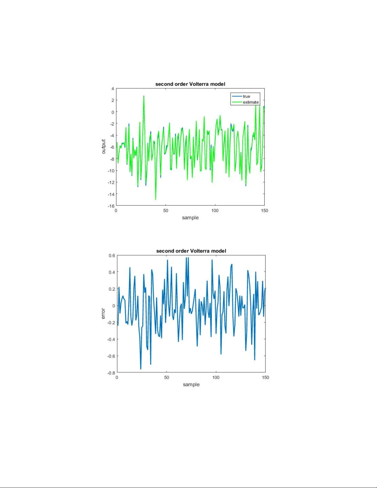
Parsimonious V olterra System Identification Sarah Hojjatinia 1 , K orkut Bekiroglu 2 , Constantino M. Lagoa 3 ∗ † ‡ § Abstract In this short paper , we aim at dev eloping algorithms for sparse V olterra system identification when the system to be identified has infinite impulse response. Assuming that the impulse response is represented as a sum of exponentials and gi ven input-output data, the problem of interest is to find the ”simplest” nonlinear V olterra model which is compatible with the a pri- ori information and the collected data. By simplest, we mean the model whose impulse response has the least number of exponentials. The algo- rithms pro vided are able to handle both fragmented data and measurement noise. Academic e xamples at the end of paper show the efficac y of proposed approach. 1 INTR ODUCTION The linear time in v ariant system identification problem has been widely addressed in the literature. There are tw o approaches for linear time inv ariant system iden- tification; set membership identification algorithms [8, 10] and subspace iden- tification algorithms [11, 12, 13]. Most techniques in parameter estimation of ∗ *This work is partially funded by the National Science F oundation (NSF) Grant CNS- 1329422. † 1 Sarah Hojjatinia is with the School of Electrical Engineering and Computer Science, The Pennsylvania State Uni versity , Univ ersity Park, P A, USA szh199@psu.edu ‡ 2 K orkut Bekiroglu is with the School of Electrical and Electronic Engineering, Nanyang T ech- nological Univ ersity , 639798 Singapore, kbekiroglu@ntu.edu.sg § 3 Constantino M. Lagoa is with F aculty of the School of Electrical Engineering and Computer Science, The Pennsylvania State Uni versity , Univ ersity Park, P A, USA lagoa@psu.edu nonlinear systems, are dependent to linearizing the system first, and then using av ailable toolboxes for linear system identification. When the data is noisy the ability to solve a nonlinear system identification becomes more dif ficult, as lin- earizing based approaches fail. Therefore, finding a method which is precise and computationally ef fectiv e is of great value. Approximating nonlinear systems with parsimonious models has the potential to be precise and computationally efficient. Sparsity in the identification of linear and nonlinear systems has been the focus of recent research. Bekiroglu et al. [2], Shah et al. [9], and Y ilmaz et al. [16] determined lo w order models from noisy input-output data for linear systems, using the concepts of sparse matrix and signal recov ery . The authors sho wed how these approaches can be applied for the case of scattered data and multiple runs of the same system with different initial conditions, for single input single output linear systems [2, 9, 16]. Bekiroglu et al. [1] e xtended the idea of low order linear system identification from noisy data, to the multiple input multiple output systems. W e extend the concept of sparse system identification to nonlinear systems. More precisely , we consider systems in the form of a V olterra series, which rep- resents a large class of nonlinear systems. There is a large body of literature on the subject of V olterra models and it mainly addresses nonlinear extensions of fi- nite impulse response (FIR) models [3]. Their structures are similar , with the first order V olterra system being a linear FIR model [7]. V olterra models are linear with respect to kernel coefficients which aids in comparison to other nonlinear models. Similar to the approaches for linear FIR models, a least squares approach can be applied to the identification of V olterra models [7]. L. Y ao, et al. [14] used least square criteria and introduced recursi ve approximation and estimation algorithm for V olterra system identification, which is dependent on the number of non-zero V olterra kernel coef ficients. 1.1 Motiv ation In contrast with pre vious work, our aim is to perform infinite impulse response identification from a finite number of noisy measurements. The objecti ve is to identify the sparsest nonlinear V olterra system which is compatible with noisy data collected and a-priori information. Algorithms provided for identifying the V olterra system aim at obtaining a compact description of the model for the infi- nite impulse response case. 1.2 Paper Outline The paper is structured as follows: after this introduction, in Section 2 formulation and structure of second order V olterra system is defined. Section 3 includes the problem statement. In Section 4 the sparse identification problem is formulated. Algorithms to tackle the problem are defined in Section 5. Numerical results are sho wn in Section 6. And finally Section 7 concludes the paper with some possible future work. 2 V OL TERRA SYSTEM For simplicity of exposition, in this paper we are going to concentrate on second order V olterra systems. Howe ver , the approach provided can readily be general- ized to higher order V olterra models. 2.1 Discr ete-time System Representation Considering x and y as the input and output of system respectiv ely , the truncated V olterra system of order 2 with L sample memory is defined as y ( n ) = h 0 + L − 1 ∑ k 1 = 0 h 1 ( k 1 ) x ( n − k 1 )+ L − 1 ∑ k 2 = 0 L − 1 ∑ k 1 = 0 h 2 ( k 1 , k 2 ) x ( n − k 1 ) x ( n − k 2 ) (1) where h 0 is a constant. h 1 and h 2 are V olterra kernel coef ficients that can be considered as impulse response and higher order system impulse response of the system. 2.2 Latrix-V ector F ormulation of V olterra System Based on [6], the first N measurements of second order V olterra system can be represented in standard matrix-vector form as y = X h (2) where y is the vector of output measurements, i.e y =  y ( 0 ) y ( 1 ) y ( N − 1 )  T , N is the total number of measurements, and X =      1 x 1 T ( 0 ) x 1 T ( 0 ) ⊗ x 1 T ( 0 ) 1 x 1 T ( 1 ) x 1 T ( 1 ) ⊗ x 1 T ( 1 ) . . . . . . . . . 1 x 1 T ( N − 1 ) x 1 T ( N − 1 ) ⊗ x 1 T ( N − 1 )      (3) where x 1 T ( n ) =  x ( n ) x ( n − 1 ) · · · x ( n − ( L − 1 ))  , ∀ n = 0 , · · · , N − 1 where ⊗ denotes the Kronecker product. h =  h 0 h T 1 h T 2  T (4) h T 1 = [ h 1 ( 0 ) h 1 ( 1 ) · · · h 1 ( L − 1 )] h 2 = vec ( H 2 ) where vec ( H 2 ) refers to v ectorized version of the matrix H 2 . H 2 =      h 2 ( 0 , 0 ) h 2 ( 0 , 1 ) · · · h 2 ( 0 , L − 1 ) h 2 ( 1 , 0 ) h 2 ( 1 , 1 ) · · · h 2 ( 1 , L − 1 ) . . . . . . . . . . . . h 2 ( N − 1 , 0 ) h 2 ( N − 1 , 1 ) · · · h 2 ( N − 1 , L − 1 )      (5) and y ∈ R N × 1 , X ∈ R N × ( 1 + L + L 2 ) , h ∈ R ( 1 + L + L 2 ) × 1 . 3 PR OBLEM ST A TEMENT 3.1 Infinite Impulse Response Repr esentation Since our objecti ve is to identify V olterra models with infinite impulse response, we represent their impulse response as a sum of exponentials. More precisely h 1 is represented as h 1 ( k 1 ) = ∑ i c 1 i a 1 i ( k 1 ) + ¯ c 1 i ¯ a 1 i ( k 1 ) (6) where c 1 i is a complex number , ¯ c 1 i is the complex conjugate of c 1 i , a 1 i ( k 1 ) is the atom which is considered as the sum of exponentials of the form: a 1 i ( k 1 ) = α i p k 1 − 1 i (7) where α i s are the scaling factors and p i s are ”poles” inside the unit circle. Also, ¯ a 1 i ( k 1 ) is the comple x conjugate of a 1 i ( k 1 ) . In a similar way , h 2 is represented as h 2 ( k 1 , k 2 ) = ∑ i c 2 i a 2 i ( k 1 , k 2 ) + ¯ c 2 i ¯ a 2 i ( k 1 , k 2 ) (8) where the atoms a 2 i ( k 1 , k 2 ) s are of the form: a 2 i ( k 1 , k 2 ) = β i p k 1 − 1 1 i p k 2 − 1 2 i (9) where β i s are the scaling factors, p 1 i and p 2 i are the ”poles”, and ¯ a 2 i ( k 1 , k 2 ) is the complex conjugate of a 2 i ( k 1 , k 2 ) . Our objectiv e is finding the second order V olterra model of the form of equa- tion (1) that uses the least possible number of exponentials. W e aim to have a simple representation of V olterra model which can be used for simulation, con- trol design and other purposes. More precisely we aim at solving the following problem. 3.2 Pr oblem Gi ven • A compact set D contained in the unit cir cle • An unknown V olterra system (2), whose impulse r esponse is a sum of e xpo- nentials whose “poles” ar e in D. • An input sequence x ( k ) , applied to system, for k = 1 , 2 , . . . , N • A noisy output sequence y η ( k ) , for k = 1 , 2 , . . . , N , given by y η ( k ) = y ( k ) + η ( k ) wher e η ( k ) denotes a noise sequence bounded by a known constant, i.e. k η ( k ) k 2 ≤ η max find the most parsimonious V olterra model which explains the input-output pair within a given bound on estimation err or ( ε ). Summarizing, we assume the exponentials in equations (7) and (9) hav e their “poles” p i , p 1 i and p 2 i in a a giv en compact set D and we aim at minimizing the number of exponentials in the representation of V olterra model while simultane- ously having a model whose response is close to the collected data. 3.3 Atomic Norm Elements of atomic set A are called atoms. The atomic norm of a model g is defined as: k g k A = inf { ∑ a 1 ∈ A ( D ) | c a 1 | + ∑ a 2 ∈ A ( D ) | c a 2 | : g = ∑ a 1 ∈ A ( D ) c a 1 a 1 + ∑ a 2 ∈ A ( D ) c a 2 a 2 } . (10) where A ( D ) is the set of atoms related to the compact set D . Every function with poles in D can be approximated as a linear combination of atoms in the set A ( D ) . A ( D ) = A 0 ( D ) ∪ A 1 ( D ) ∪ A 2 ( D ) A 0 ( D ) = { a 0 = 1 , a 1 i ( k 1 ) = 0 , a 2 i ( k 1 , k 2 ) = 0 } A 1 ( D ) = { a 0 = 0 , a 1 i ( k 1 ) = α i p k − 1 i , a 2 i ( k 1 , k 2 ) = 0 : ∀ p i ∈ D } A 2 ( D ) = { a 0 = 0 , a 1 i ( k 1 ) = 0 , a 2 i ( k 1 , k 2 ) = β i p k 1 − 1 1 i p k 2 − 1 2 i : ∀ p 1 i , p 2 i ∈ D } (11) 3.4 Higher Order V olterra Models In this part we giv e some insight toward the generalization of proposed approach to higher order V olterra models. In general, the V olterra system is in the form of y ( n ) = h 0 + · · · + ∞ ∑ k 1 = 0 . . . ∞ ∑ k m = 0 h m ( k 1 , . . . , k m ) m ∏ i = 1 x ( n − k i ) + . . . (12) where h 0 is a constant, and h m s , ∀ m = 1 , · · · , ∞ are V olterra kernel coef ficients. Applicable V olterra systems are truncated to some predefined order . The truncated V olterra system of order m with L sample memory is defined as y ( n ) = h 0 + · · · + L − 1 ∑ k 1 = 0 . . . L − 1 ∑ k m = 0 h m ( k 1 , . . . , k m ) m ∏ i = 1 x ( n − k i ) (13) where for m = 1, the V olterra system is a linear system. By considering m ≥ 2 the V olterra system represents a nonlinear system. For V olterra system of order m , kernel coefficient h m ( k 1 , . . . , k m ) will be defined in the same way of equations (8) and (9). h m ( k 1 , . . . , k m ) = ∑ i c mi a mi (( k 1 , . . . , k m ) + ¯ c mi ¯ a mi (( k 1 , . . . , k m ) (14) where the atoms a mi (( k 1 , . . . , k m ) s are of the form: a mi (( k 1 , . . . , k m ) = ζ i P k 1 − 1 1 i P k 2 − 1 2 i · · · P k m − 1 mi (15) where ζ i s are the scaling factors, P 1 i , P 2 i , · · · , and P mi are the poles. Therefore, in a similar way we can formulate problem for higher order V olterra systems and apply the approach in this paper to identify the parsimonious model. 4 FORMULA TION OF THE SP ARSE IDENTIFI- CA TION PR OBLEM As mentioned in the Introduction, in the identification of systems, whether lin- ear or nonlinear , the concept of “parsimonious representation” plays an important role. K ekatos and Giannakis [5] introduced compressed sampling approaches, in parsimonious identification of V olterra and polynomial models. Y ilmaz et al. [15] introduced an algorithm for parsimonious linear system identification; specif- ically , it is a randomized algorithm which minimize a con vex function over an atomic set; atomic set is considered to be scaled ball. In this paper we extend the idea of sparse system identification for the case of nonlinear systems. The problem of interest of this paper , parsimonious identification of V olterra models with infinite impulse response, can be formulated as min c cardinality { c 6 = 0 } s.t.   y η − X h   2 2 ≤ ε equations ( 4 ) , ( 6 ) , and ( 8 ) (16) where c is a vector containing all coef ficients, and y η is the vector of noisy mea- surements, i.e. y η = y + η and η is noise η =  η ( 0 ) η ( 1 ) η ( N − 1 )  T . Also, the matrix X , as in equation (3), is a structured matrix containing input v alues, and h is a vector containing the first fe w entries of the impulse response. Again, in the proposed approach, h is assumed to be representable by a sum of exponentials. More precisely , it has the form gi ven by equations (4), (6), and (8). c i s are complex coef ficients. Remark 1 This optimization pr oblem can be r eadily modified to handle missing measur ements. The first constraint in equation (16) can be r eplaced by   y η − X h   2 2 ≤ ε at the times when we have measurements. Minimizing cardinality subject to constraints is an NP-hard problem. It makes us to think about the relaxation of original optimization problem in equation (16) and using atomic norm. 5 ALGORITHMS T O SOL VE THE PR OBLEM For solving or approximating the solution of the complex optimization problem in equation (16), sev eral algorithms are suggested in this section. Therefore, the parsimonious V olterra system identification problem in (16) can be approximated by: 1. Grid the set of atoms. One can do a griding of the set of poles as depicted in Figure 1 for poles p i , p 1 i and p 2 i . Then, solve the mixed integer optimization problem min ∑ i σ i s.t. σ i ∈ { 0 , 1 } | c i | ≤ M σ i equations ( 4 ) , ( 6 ) , and ( 8 ) (17) where c i is the coeffici ent associated with the exponential whose “pole” is the i -th element of the grid and M is an upper bound on the maximum v alue of | c i | . This algorithm is again NP-hard. Hence, two l 1 relaxations of the algorithm are introduced as follo ws: 2. Griding the set of atoms as abov e and using l 1 norm relaxation of cardinality to obtain k c k 1 sparse, as a surrogate of cardinality { c : c 6 = 0 } min h k h k A s.t.   y η − X h   2 2 ≤ ε equations ( 4 ) , ( 6 ) , and ( 8 ) (18) 3. Again, using l 1 as a surrogate of cardinality , the randomized version of Frank-W olfe algorithm that was dev eloped in [15]; can be readily adapted to deal with the problem in this paper . More precisely , one can use a ran- domized Frank-W olfe algorithm to solv e the problem min h   y η − X h   2 2 s.t. k h k A ≤ τ equations ( 4 ) , ( 6 ) , and ( 8 ) (19) This approach has much less computational complexity than the other two. Ho wev er , a closed form representation of the impulse response will not be obtained. As a result, an additional step needs to be performed to identify the exponentials that are present in the identified impulse responses. 6 NUMERICAL RESUL TS In the examples to follo w , we solv e the problem of sparse V olterra system identifi- cation with the l 1 norm relaxation. More precisely , we use algorithm 2 in Section 5. Note that in using l 1 norm relaxation, scalings of the atoms ( α i and β i ) play a significant role on ho w sparse the solution can be and further research is needed to determine the “optimal” scaling v alues. In the numerical examples presented, N measurements are considered. Ran- dom measurement noise is added to true outputs. The unit circle has been gridded uniformly and random poles were picked to check as candidates for the system. Figure 1: A sample of griding the unit circle. CVX is used as the con vex optimization toolbox [4]. In this paper we use scaling factors α i = 1 and β i = 1. Example one relates to a second order V olterra system, which is generated at random as a sum of 4 exponentials. Random poles and coefficients selected for this algorithm are sho wn in T able 1. A random uniform measurement noise with the maximum v alue, approximately 11 . 2% of the mean absolute v alue of outputs, is added. Number of measurements is considered to be N = 100 in this example. Impulse response of the estimated model ( h 2 ) compared to the true one is plotted in Figure 2. The true and estimated output are sho wn in Figure 3; by true output we mean the output before adding noise. The dif ference between true and estimated output is shown in Figure 4. The estimated model is a sum of 5 exponentials, which sho ws a sparse identification of system. Therefore, having optimal v alues for the scalings α i and β i , would result in the true sparse system. Figure 2: True and estimated impulse response in second order V olterra system, example 1. Figure 3: True and estimated output in second order V olterra system, e xample 1. T able 1: Random selection of poles and coefficients for e xample 1. First order poles First order coefficients Second order poles 1 p i ∀ i = 1 , · · · , 4 c 1 i ∀ i = 1 , · · · , 4 p 1 i ∀ i = 1 , · · · , 2 -0.1375 + j 0.2731 1.8969 + j 0.0618 0.2270 + j 0.1086 -0.1210 + j 0.3591 0.2834 -j 0.6773 0.4978 - j 0.4239 0.7844 + j 0.0577 1.9874 - j 0.2800 -0.8890 - j 0.2277 0.2142 - j 0.0328 Second order poles 2 Second order coefficients p 2 i ∀ i = 1 , · · · , 2 c 2 i ∀ i = 1 , · · · , 2 0.3591 - j 0.6873 1.5449 - j 1.2369 -0.7062 + j 0.5511 1.7244 - j 0.9657 Figure 4: Difference between true and estimated output in second order V olterra system, example 1. Example two relates to identification of a second order V olterra model with N = 150 measurements. Random poles and coefficients selected for this algo- rithm are shown in T able 2. Random measurement noise with the maximum v alue, approximately 8% of the mean absolute value of outputs is added. The corresponding poles and coef ficients for this model are as T able 2. T able 2: Random selection of poles and coefficients for e xample 2. First order poles First order coefficients Second order poles 1 p i ∀ i = 1 , · · · , 4 c 1 i ∀ i = 1 , · · · , 4 p 1 i ∀ i = 1 , · · · , 2 -0.6019 + j 0.2180 -1.9283 - j 1.8763 0.3966 + j 0.6776 0.4813 - j 0.4971 -1.5213 - j 0.0245 0.0182 + j 0.0431 0.1924 - j 0.3459 1.8085 + j 1.4509 0.8084 -j 0.0051 1.9034 - j 1.0285 Second order poles 2 Second order coefficients p 2 i ∀ i = 1 , · · · , 2 c 2 i ∀ i = 1 , · · · , 2 -0.5943 - j 0.5600 0.5278 + j 0.2857 0.5027 + j 0.3444 -1.0269 + j 1.9269 Figure 5 shows the impulse response of the estimated model ( h 2 ) compared to the true one. The true and estimated outputs of second order V olterra system are depicted in Figure 6. The difference between estimated and true outputs is sho wn in Figure 7. As illustrated in the figures, the output of nonlinear system has been approx- imated efficiently . The impulse response shows good con vergence. Coef ficients of the identified V olterra model are close to the coefficients of true system. As a result, the sparsity has been achie ved. 7 CONCLUSION AND FUTURE WORK In this paper , we provide a novel approach to the problem of identifying parsi- monious models for nonlinear V olterra systems with infinite impulse response. Gi ven noisy fragmented input-output data, we identify the “simplest” nonlinear model which best describes the data. The performance of the proposed approach is illustrated in two academic e xamples. W e believ e the proposed method is useful in parsimonious V olterra system identification and control problems. In cases which we do not hav e much prior Figure 5: True and estimated impulse response in second order V olterra system, example 2. kno wledge of system rather than the noisy collected data, this method provides an ef ficient way to estimate a model. Effort is now being put in the de velopment of ef ficient algorithms that can both handle large amounts of data and do not require the large number of v ariables that occur when using griding. Refer ences [1] K orkut Bekiroglu, C Lagoa, and Mario Sznaier . Low-order model identifi- cation of mimo systems from noisy and incomplete data. In Decision and Contr ol (CDC), 2015 IEEE 54th Annual Confer ence on , pages 4029–4034. IEEE, 2015. [2] K orkut Bekiroglu, Burak Y ilmaz, C Lagoa, and Mario Sznaier . Parsimo- nious model identification via atomic norm minimization. In Contr ol Con- fer ence (ECC), 2014 Eur opean , pages 2392–2397. IEEE, 2014. Figure 6: True and estimated output in second order V olterra system, e xample 2. Figure 7: Difference between true and estimated output in second order V olterra system, example 2. [3] Grard Fa vier , Alain Y . Kibangou, and Thomas Bouilloc. Nonlinear sys- tem modeling and identification using volterra-parafac models. International J ournal of Adaptive Contr ol and Signal Pr ocessing , 26(1):30–53, 2012. [4] Michael Grant and Stephen Boyd. CVX: Matlab software for disciplined con ve x programming, version 2.1. [5] V . Kekatos and G. B. Giannakis. Sparse volterra and polynomial regres- sion models: Recov erability and estimation. IEEE T ransactions on Signal Pr ocessing , 59(12):5907–5920, Dec 2011. [6] V John Mathews and Giov anni L Sicuranza. P olynomial signal pr ocessing , volume 27. W iley-Interscience, 2000. [7] Michael Nikolaou and Diwakar Mantha. Efficient Nonlinear Modeling Using W avelet Compr ession , pages 313–334. Birkh ¨ auser Basel, Basel, 2000. [8] Ricardo S Sanchez-Pena and Mario Sznaier . Rob ust systems theory and ap- plications . John W iley & Sons, Inc., 1998. [9] Parikshit Shah, Badri Narayan Bhaskar , Gongguo T ang, and Benjamin Recht. Linear system identification via atomic norm regularization. In De- cision and Contr ol (CDC), 2012 IEEE 51st Annual Confer ence on , pages 6265–6270. IEEE, 2012. [10] Mario Sznaier . Control-oriented system identification: An h ∞ approach, jie chen and guoxiang gu, wiley , ne w york, 2000, 421 p. isbn 0-471-32048- x. International J ournal of Robust and Nonlinear Contr ol , 13(5):497–498, 2003. [11] Peter V an Overschee and Bart De Moor . Subspace algorithms for the stochastic identification problem. Automatica , 29(3):649–660, 1993. [12] Peter V an Overschee and Bart De Moor . N4sid: Subspace algorithms for the identification of combined deterministic-stochastic systems. Automatica , 30(1):75–93, 1994. [13] Peter V an Overschee and BL De Moor . Subspace identification for linear systems: Theory- Implementation- Applications . Springer Science & Busi- ness Media, 2012. [14] L. Y ao, W . A. Sethares, and Y . H. Hu. Identification of a nonlinear system modeled by a sparse volterra series. In [Pr oceedings 1992] IEEE Interna- tional Confer ence on Systems Engineering , pages 624–627, Sep 1992. [15] B. Y ilmaz, K. Bekiroglu, C. Lagoa, and M. Sznaier . A randomized algo- rithm for parsimonious model identification. IEEE T ransactions on Auto- matic Contr ol , PP(99):1–1, 2017. [16] Burak Y ilmaz, C Lagoa, and Mario Sznaier . An efficient atomic norm min- imization approach to identification of low order models. In Decision and Contr ol (CDC), 2013 IEEE 52nd Annual Confer ence on , pages 5834–5839. IEEE, 2013.