Connectionist Temporal Localization for Sound Event Detection with Sequential Labeling

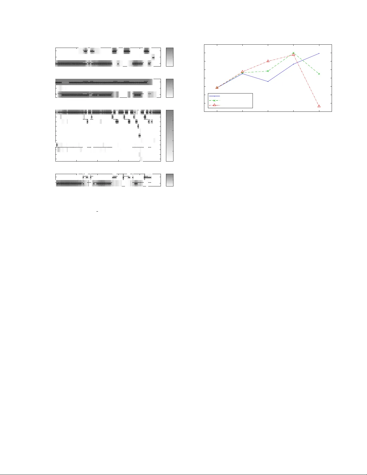
CONNECTIONIST TEMPORAL LOCALIZA TION FOR SOUND EVENT DETECTION WITH SEQUENTIAL LABELING Y un W ang and Florian Metze Language T echnologies Institute, Carnegie Mellon Uni versity , Pittsbur gh, P A, U.S.A. maigoakisame@gmail.com, fmetze@cs.cmu.edu ABSTRA CT Research on sound ev ent detection (SED) with weak labeling has mostly focused on presence/absence labeling, which provides no temporal information at all about the ev ent occurrences. In this paper , we consider SED with sequential labeling, which specifies the temporal order of the event boundaries. The con ventional con- nectionist temporal classification (CTC) framew ork, when applied to SED with sequential labeling, does not localize long e vents well due to a “peak clustering” problem. W e adapt the CTC framew ork and propose connectionist temporal localization (CTL), which suc- cessfully solves the problem. Evaluation on a subset of Audio Set shows that CTL closes a third of the gap between presence/absence labeling and strong labeling, demonstrating the usefulness of the extra temporal information in sequential labeling. CTL also makes it easy to combine sequential labeling with presence/absence labeling and strong labeling. Index T erms — Sound event detection (SED), weak labeling, sequential labeling, connectionist temporal classification (CTC) 1. INTR ODUCTION Sound e vent detection (SED) is the task of classifying and localizing occurrences of sound ev ents in audio streams. The training of SED models used to rely upon str ong labeling , which specifies the type, onset time and of fset time of each sound event occurrence. Such labeling, howe ver , is very tedious to obtain by hand. In order to scale SED up, many successful attempts have been made to train SED systems with weak labeling , such as [ 2 , 3 , 4 ] and our T ALNet [ 5 ]. Even though trained with weak labeling, some of these systems are able to temporally localize ev ents in their output. When the term weak labeling is used in the literature, it often specifically refers to pr esence/absence labeling , which only specifies the types of sound events present in a recording b ut does not provide any temporal information. Presence/absence labeling is popular because it takes the least effort to produce; as such, Audio Set [ 6 ], the currently largest corpus for SED, is also labeled this way . In this paper , ho wever , we study SED with sequential labeling, which specifies the order of the boundaries of events occurring in each recording. W e demonstrate that the extra temporal information in sequential labeling, though incomplete, can still improve the localization of sound ev ents. Connectionist temporal classification (CTC) [ 7 ] is a popular framew ork used for speech recognition when the supervision is sequential, e.g . phoneme sequences without temporal alignment [ 8 ]. CTC has been directly applied to SED with sequential labeling in [ 9 ] and a pre vious work of ours [ 10 ]; the latter found that a “peak This work was supported in part by a gift aw ard from Robert Bosch LLC and a faculty research aw ard from Google. It used the “comet” and “bridges” clusters of the XSEDE en vironment [ 1 ], supported by NSF grant number ACI-1548562. clustering” problem impeded the accurate localization of long sound ev ents. In this paper, we make three major modifications to CTC and propose a connectionist temporal localization (CTL) frame work, which successfully solves the peak clustering problem. Evaluation on a subset of Audio Set sho ws that CTL closes a third of the gap between presence/absence labeling and strong labeling. Our CTL frame work also pro vides a way to easily combine mul- tiple types of labeling, such as presence/absence labeling, sequential labeling, and strong labeling. When we have stronger labeling av ailable in a smaller amount and weaker labeling av ailable in a larger amount, such a combination makes it possible to fully exploit the information in all the data. 2. CTL: MOTIV A TION AND ALGORITHM 2.1. Sequential Labeling In speech recognition, a typical form of supervision is a phoneme sequence for each utterance without temporal alignment. A direct analogy for SED would be a sequence of sound events for each recording, but the order of sound ev ents can be hard to define when they overlap. T o a void this problem, we define sequential labeling to be a sequence of e vent boundaries. For example, if the content of a recording can be described as “a dog barks while a car passes by”, the sequence of e vent boundaries will be: car onset, dog onset, dog offset, car offset. W e denote this by ´ C ´ D ` D ` C : letters with the rising accent ´ C , ´ D stand for the onsets of the “car” and “dog” e vents, while letters with the falling accent ` C and ` D stands for their offsets; the underline means this is a sequence without temporal alignment. For annotators, sequential labeling is not too much harder to produce than presence/absence labeling; the difficulty mainly arises when sound ev ents occur densely or overlap. In any case, it is still easier to produce than strong labeling, because it is not necessary to mark the precise onset and of fset times of each sound event occurrence. Also, sequential labeling may be automatically mined from textual descriptions of audio recordings, such as “a dog barks while a car passes by”. 2.2. The Peak Clustering Problem of CTC CTC can be applied to SED with sequential labeling as follows. First, we define the vocab ulary of CTC output to include the onset and offset labels of each e vent type, plus a “blank” label (denoted by - ). For an SED system that deals with n types of events, the vocab ulary size is 2 n + 1 . A neural network (often with a recurrent layer) predicts the frame-wise probability of each label in the vocab- ulary; these probabilities sum to 1 at each frame. The probabilities of specific temporal alignments ( e.g. - ´ C ´ D ` D ` C- , ´ C- ´ D ` D ` C ` C ) can be calculated by multiplying the probabilities of individual labels at each frame. The total probability of the ground truth sequence ( e.g . ´ C ´ D ` D ` C ) is defined as the sum of the probabilities of all alignments that can be reduced to the ground truth sequence by a many-to-one mapping B ; this mapping first collapses all consecutive repeating labels into a single one, then removes all blank labels. For example, both the alignments - ´ C ´ D ` D ` C- and ´ C- ´ D ` D ` C ` C can be reduced to the unaligned sequence ´ C ´ D ` D ` C , therefore P ( ´ C ´ D ` D ` C ) = P ( - ´ C ´ D ` D ` C- ) + P ( ´ C- ´ D ` D ` C ` C ) plus the probabilities of many other alignments. A systematic forward algorithm is proposed in [ 7 ] to compute this total probability ef ficiently . The loss function for this recording is defined as − log P ( ´ C ´ D ` D ` C ) ; this can be minimized with any neural network training algorithm, such as gradient descent. When CTC is directly applied to SED with sequential labeling, it has been found in [ 10 ] to detect short events well: a peak appears in the frame-wise probabilities of the onset and of fset labels around the actual occurrence of the e vent. For long ev ents, howe ver , CTC tends to predict peaks for the onset and the of fset next to each other , which means the ev ent is not well localized (see Sec. 3.3 for an example). This “peak clustering” problem occurs for se veral reasons. First, because sound ev ents do not ov erlap too often, adjacent onset and offset labels are an extremely common pattern in the training label sequences. As a result, CTC may misunderstand a pair of onset and offset labels as collectively indicating the existence of an event, instead of understanding them as separately indicating the e vent boundaries. Second, the CTC loss function only mandates the order of the predicted labels, without imposing any temporal constraints. In this case, the recurrent layer of the network will prefer to emit onset and offset labels next to each other , because this minimizes the effort of memory . The root cause of the “peak clustering” problem is that the output layer of the network is only trained to detect event boundaries ; it is expected to keep “silent” both when an ev ent is inactiv e and when an ev ent is continuing, despite the potentially huge dif ferences in the acoustic features. When the network predicts the onset and offset labels of a long ev ent occurrence next to each other , it actually does not violate this expectation on too many frames, and does not hav e enough incentive to correct this beha vior . 2.3. Connectionist T emporal Localization In this section we make three major modifications to the CTC framew ork, and present a connectionist temporal localization (CTL) framew ork suitable for localizing sound e vents. W e also describe the corresponding forward algorithm for calculating the total probability of an ev ent boundary sequence. The first modification addresses the root cause of the “peak clustering” problem: the output layer of the network should predict the frame-wise pr obabilities of the events themselves instead of those of the event boundaries . In this way , the network can learn to make different predictions with different acoustic features. The boundary probabilities are then deriv ed from the ev ent probabilities using a “rectified delta” operator . More formally , let y t ( E ) be the probability of the event E being active at frame t . Here 1 ≤ t ≤ T , where T is the number of frames in the recording in question. Let z t ( ´ E ) and z t ( ` E ) be the probabilities of the onset and of fset labels of the event E at frame t . W e calculate them using the following equations: z t ( ´ E ) = max[0 , y t ( E ) − y t − 1 ( E )] z t ( ` E ) = max[0 , y t − 1 ( E ) − y t ( E )] (1) In these equations we allow t to range from 1 to T + 1 , in order to accommodate ev ents that start at the first frame or end at the last frame. When y 0 ( E ) or y T +1 ( E ) is referenced, we assume it to be 0. Now we have the frame-wise probabilities of all ev ent bound- aries, we only need to define the frame-wise probability of the blank. Howe ver , a difficulty arises because the sum of the boundary probabilities at a given frame may exceed 1. T o solve this problem, we make the second modification to CTC: we treat the pr obabilities of differ ent event boundaries at the same frame as mutually indepen- dent, instead of mutually exclusive . In this way , the probability of no ev ent boundaries occurring at frame t can be calculated by:  t = Y l [1 − z t ( l )] (2) where l goes over all e vent boundaries. The probability of emitting a single ev ent boundary l at frame t is then: p t ( l ) = z t ( l ) · Y l 0 6 = l [1 − z t ( l 0 )] (3) If we define δ t ( l ) = z t ( l ) 1 − z t ( l ) (4) Then Eq. 3 reduces to p t ( l ) =  t · δ t ( l ) (5) The assumption that boundary labels at the same frame are mutually independent seems to eliminate the need for the blank label. Indeed, the blank label in CTC serves two purposes: (1) to allow emitting nothing at a frame, and (2) to separate consecuti ve repetitions of the same label. W ith the independence assumption, the first purpose is naturally achiev ed. Here we make the third modification to CTC: the mapping B no longer collapses consecutive r epeating labels into a single one . W ith this simplification, the blank label can be remov ed altogether . The independence assumption also allo ws us to assess the prob- ability of emitting multiple labels at the same frame, which is not possible with the standard CTC. The probability of emitting multiple labels l 1 , . . . , l k together at frame t can be calculated as p t ( l 1 , . . . , l k ) = Y k i =1 z t ( l i ) · Y l / ∈{ l 1 ,...,l k } [1 − z t ( l )] =  t · Y k i =1 δ t ( l i ) (6) Now we can formulate our CTL forward algorithm. What we want to find is the total probability of emitting the ground truth label sequence L = l 1 , . . . , l | L | , regardless of the temporal alignment. What we are giv en is the frame-level probabilities of events y t ( E ) , from which we can deriv e the probability p t ( · ) of emitting zero, one or more labels at each frame by Eq. 6 . Let α t ( i ) be the probability of having emitted exactly the first i labels of L after t frames. The α ’ s can be computed with the following recurrence formula: α t ( i ) = X i j =0 α t − 1 ( i − j ) · p t ( l i − j +1 , . . . , l i ) = X i j =0 α t − 1 ( i − j ) ·  t · Y i k = i − j +1 δ t ( l k ) (7) In the summation, the index j stands for the number of labels emi tted at frame t . The initial values are: α 0 ( i ) =  1 , if i = 0 0 , if i > 0 (8) The final value, α T +1 ( | L | ) , is the total probability of emitting the label sequence L , and its negativ e logarithm is the contribution of the recording in question to the loss function. Eq. 7 allows emitting arbitrarily many labels at the same frame. When the ground truth label sequence is long, this can pose a prob- lem of time complexity . In practice, it is rare for multiple labels to be emitted at the same frame. Therefore, it can be desirable to limit the maximum number of concurrent labels, i.e. the maximum value of j in Eq. 7 . W e call this maximum v alue the max concurrence . 400 * 64 * 16 conv 3* 3 Filterbank features 200 * 3 2 * 16 pool 2*2 200 * 32 * 32 conv 3* 3 100 * 16 * 3 2 pool 2*2 100 * 16 * 64 conv 3* 3 100 * 8 * 64 pool 1*2 100 * 8 * 128 conv 3* 3 100 * 4 * 1 28 pool 1*2 100 * 4 * 256 conv 3* 3 100 * 512 flatten 100 * 512 BiGRU 256*2 1 * 3 5 Recording-le vel probabilities of events 400 * 64 * 1 (b) MIL sys te m for presence/abse nce labeling 100 * 2 * 256 pool 1*2 100 * 2 * 5 12 conv 3* 3 100 * 1 * 512 pool 1*2 100 * 3 5 100 * 3 5 Frame-level prob abil ities of events 100 * 71 Frame-level probabilities of event boundaries 100 * 35 101 * 70 Rectified delta Linear softmax (a) Strong labeling system (c) CTC sys tem for sequential labeling (d) CTL s ystem f or sequential labeling Fully connected (sigmoid) Frame-level p robabilities of events Frame-level proba b ilities of events Frame-level proba b ilities of event boundari e s Fig. 1 . Structures of the four networks trained in Sec. 3.2 . The shape is specified as “frames * frequency bins * feature maps” for 3-D tensors (shaded), and “frames * feature maps” for 2-D tensors. “con v n * m ” stands for a con volutional layer with the specified kernel size and ReLU activ ation; batch normalization is applied before the ReLU activ ation. “pool n * m ” stands for a max pooling layer with the specified stride. 3. EXPERIMENTS 3.1. Data Preparation W e carried out experiments on a subset of Audio Set [ 6 ]. Audio Set consists of ov er 2 million 10-second excerpts of Y ouT ube videos, labeled with the presence/absence of 527 types of sound events. Because we would need sequential labeling for training and strong labeling for evaluation, we generated sequential and strong labeling for all the recordings using T ALNet [ 5 ] – a state-of-the-art network trained with presence/absence labeling that is good at localizing sound ev ents. W e used a frame length of 0.1 s, so each recording consisted of 100 frames. Not all of the 527 sound ev ents types of Audio Set were labeled with high quality , and the labels generated by T ALNet would be ev en noisier . T o reduce the ef fect of such label noise, we selected 35 sound ev ent types that had relati vely reliable labels (see T able 4.1 of [ 11 ] for a complete list). Four of these ev ent types ( speech , sing , music and crowd ) were ov erwhelmingly frequent; we fil- tered the recordings of Audio Set to retain only those that contained at least one of the remaining 31 types of sound events. This left us with 359,741 training recordings, 4,879 validation recordings and 5,301 ev aluation recordings. The total duration of these recordings is around 1,000 hours, or 18% of entire corpus. 3.2. Network Structures and T raining W e trained four networks whose structures are illustrated in Fig. 1 . All the layers up to the GRU layer are shared across the four net- works; these layers highly resemble the hidden layers of T ALNet [ 5 ], but are shallo wer and narrower . The four systems ha ve dif ferent out- put ends. The first system predicts the probabilities of the 35 types of sound ev ents, and directly receiv es strong labeling as supervision. The second system is a multiple instance learning (MIL) system for presence/absence labeling: it first predicts frame-wise probabilities, then aggregates them into recording-level probabilities with a linear softmax pooling function just like T ALNet. These two systems serv e as the topline and the baseline for the CTC and CTL systems. The CTC system directly predicts the frame-wise probabilities of ev ent boundaries and the blank label; the output layer has 35 ∗ 2 + 1 = 71 System Loc. F 1 (%) Strong labeling (topline) 67.38 MIL (baseline) 55.83 CTC 31.91 CTL Max concurrence = 1 59.92 Max concurrence = 2 57.49 Max concurrence = 3 53.63 T able 1 . Localization performance of the four systems. units. The CTL system predicts the frame-wise probabilities of the ev ents and then deriv es the boundary probabilities with the “rectified delta” operator . W e tried max concurrence values of 1, 2 and 3. The systems were trained using the Adam optimizer [ 12 ] with a constant learning rate of 10 − 3 . The batch size was 500 recordings. W e applied data balancing to ensure that each minibatch contained roughly equal numbers of recordings of each ev ent type. After e very 200 minibatches (called a chec kpoint ), we ev aluated the network’ s localization performance using the frame-level F 1 macro-av eraged across the 35 ev ent types. F or the strong labeling, MIL and CTL systems, we first tuned class-specific thresholds to optimize the frame-lev el F 1 of each ev ent type on the validation data, then applied them directly to the ev aluation data. For the CTC system, we picked the most probable label at each frame, and marked each event as activ e between innermost matching pairs of onset and offset labels. 3.3. Perf ormance of CTL for Sequential Labeling T able 1 lists the highest ev aluation F 1 obtained by the various sys- tems within 100 checkpoints. The CTC system f alls long behind the baseline; as we shall see, this is due to the “peak clustering” problem. The CTL system (with a max concurrence of 1) successfully outper - forms the baseline, and closes a third of the gap between the baseline of MIL with presence/absence labeling and the topline of strong labeling. A class-wise error analysis shows that the CTL system exhibits a uniform improvement across classes, outperforming the MIL baseline for 28 of the 35 ev ent types. In addition, it appears unnecessary to allow multiple labels to occur at the same frame. Fig. 2 presents the output of the four systems on an ev aluation recording, which contains the whining of a dog intermingled with 0 2 4 6 8 10 speech child dog Event (a) Strong labeling system 0 0.5 1 0 2 4 6 8 10 speech music dog Event (b) MIL system 0 0.5 1 0 2 4 6 8 10 blank Label (c) CTC system 0 0.2 0.4 0.6 0.8 1 0 2 4 6 8 10 Time (s) speech dog Event (d) CTL system 0 0.5 1 Fig. 2 . The frame-le vel predictions of the four systems on the ev aluation recording 0F04c rY4aw . Dots stand for the ground truth; shades of gray indicate the frame-lev el probabilities of ev ents, ev ent boundaries or the blank label. Crosses indicate the most probable label at each frame (for the CTC system), or ev ents with probabilities higher than the class-specific thresholds (for the other systems). and stand for the onset and offset labels of the ev ent E . Unimportant events are omitted. speech. The topline strong labeling system localizes both ev ents well; the baseline MIL system fails to localize the speech ev ent. The CTC system can localize the occurrences of speech (although with a fe w spurious detections); for the dog event, howe ver , it exhibits the “peak clustering” problem: it predicts (with low con- fidence) many pairs of onset and offset labels of dog next to each other . The CTL system avoids the “peak clustering” problem, and also localizes the speech occurrences better than the MIL system. 3.4. Combining Sequential Labeling with Presence/Absence La- beling When sequential labeling is av ailable for training a SED system, presence/absence labeling is automatically also av ailable. This prompts us to think about combining a CTL system trained with sequential labeling and an MIL system trained with presence/ absence labeling. Because the two systems share all layers up to the frame-wise probabilities of events, this combination turns out to be surprisingly easy: it suffices to combine the loss functions of the two systems using a weighted average. At test time, the localization output can be directly taken from the shared layer of frame-wise ev ent probabilities. In contrast, it is more dif ficult to combine a CTC system with an MIL system because the y hav e dif ferent output ends. W e combined an MIL system with CTL systems trained with different values of max concurrence: 1, 2 and 3. When we trained the systems alone, we found that the loss of the CTL systems usually stabilized around 0.2, while the loss of the MIL system usually stabilized around 0.02. F or the combination experiments, Pure MIL 30:1 10:1 3.3:1 Pure CTL 53 54 55 56 57 58 59 60 61 Macro-average frame-level F1 (%) max concurrence = 1 max concurrence = 2 max concurrence = 3 Fig. 3 . The localization performance obtained by combining CTL and MIL with different weights. we fixed the weight of the CTL loss to 1, and tried out the following weights for the MIL loss: 30 (emphasizing the MIL loss more), 10 (weighting both losses equally), and 3.3 (emphasizing the CTL loss more). The resulting localization performances are plotted in Fig. 3 . A mixing weight of 3.3:1 appears to be generally a good choice, and giv es a marginal improv ement on top of pure CTL. The potential use of combining a CTL system with other systems is not limited to the experiments abov e. Because sequential labeling takes more effort to produce than presence/absence labeling after all, it can be well imagined that there will be less data with sequential labeling av ailable than data with presence/absence labeling. System combination allows us to exploit the information in both types of labeling: we can compute the MIL loss on all the data and the CTL loss on the part of the data with sequential labeling, and train a system to minimize an appropriate weighted average of the tw o loss functions. If we also have data with strong labeling, then the frame- wise cross-entropy loss of a strong labeling system can be added to the weighted a verage, too. A CTL system can be combined with an MIL system and a strong labeling system with no effort, thanks to the fact that it computes frame-wise probabilities of events in the same way as the other two systems. 4. CONCLUSION AND DISCUSSION W e made three modifications to the connectionist temporal clas- sification (CTC) framework: (1) instead of predicting frame-wise boundary probabilities directly , the network predicts ev ent proba- bilities and then derives boundary probabilities using a “rectified delta” operator; (2) the boundary probabilities at the same frame are regarded as mutually independent instead of mutually exclusiv e; (3) the mapping B from alignments to unaligned label sequences no longer collapses consecutive repeating labels. The resulting framew ork, which we name “connectionist temporal localization” (CTL), successfully solves the “peak clustering” problem of CTC, and closes a third of the gap between the baseline of presence/ absence labeling and the topline of strong labeling. Because a CTL system predicts frame-wise e vent probabilities in the same way as an MIL system for presence/absence labeling and a strong labeling system, the combination of the three systems is as easy as a weighted average of the loss functions. This makes it possible to exploit the information in all three types of labeling when we hav e different data labeled at dif ferent granularities. For more details about the CTL algorithm and the experiments, please refer to Chapter 4 of the first author’ s PhD thesis [ 11 ]. The code and acoustic features for the experiments are av ailable at https://github.com/MaigoAkisame/cmu- thesis . 5. REFERENCES [1] J. T owns, T . Cockerill, M. Dahan, I. Foster , K. Gaither, A. Grimshaw, V . Hazlew ood, S. Lathrop, D. Lifka, G. D. Peterson, R. Roskies, J. R. Scott, and N. Wilkins-Diehr, “XSEDE: Accelerating scientific discovery , ” Computing in Science & Engineering , vol. 16, no. 5, pp. 62–74, 2014. [2] S. Hershey et al. , “CNN architectures for large-scale audio classifica- tion, ” in International Conference on Acoustics, Speech, and Signal Pr ocessing (ICASSP) , IEEE, 2017, pp. 131–135. [3] Q. Kong, Y . Xu, W . W ang, and M. D. Plumbley , “ Audio set clas- sification with attention model: A probabilistic perspective, ” in In- ternational Confer ence on Acoustics, Speech, and Signal Processing (ICASSP) , IEEE, 2018, pp. 316–320. [4] C. Y u, K. S. Barsim, Q. K ong, and B. Y ang, “Multi-level attention model for weakly supervised audio classification, ” ArXiv e-prints , 2018. [Online]. A vailable: http : / / arxiv . org / abs / 1803 . 02353 . [5] Y . W ang, J. Li, and F . Metze, “A comparison of five multiple instance learning pooling functions for sound ev ent detection with weak labeling, ” ArXiv e-prints , 2018. [Online]. A vailable: http : //arxiv.org/abs/1810.09050 . [6] J. F . Gemmeke, D. P . W . Ellis, D. Freedman, A. Jansen, W . Lawrence, R. C. Moore, M. Plakal, and M. Ritter, “Audio Set: An ontology and human-labeled dataset for audio events, ” in International Confer ence on Acoustics, Speech, and Signal Processing (ICASSP) , IEEE, 2017, pp. 776–780. [7] A. Graves, S. Fern ´ andez, F . Gomez, and J. Schmidhuber, “Con- nectionist temporal classification: Labelling unsegmented sequence data with recurrent neural networks, ” in International Confer ence on Machine Learning (ICML) , A CM, 2006, pp. 369–376. [8] A. Graves and N. Jaitly, “T owards end-to-end speech recognition with recurrent neural networks, ” in International Conference on Machine Learning (ICML) , A CM, 2014, pp. 1764–1772. [9] Y . Hou, Q. Kong, J. W ang, and S. Li, “Polyphonic audio tagging with sequentially labelled data using crnn with learnable g ated linear units, ” in Pr oceedings of the Detection and Classification of Acoustic Scenes and Events 2017 W orkshop (DCASE2017) , 2018, pp. 78–82. [10] Y . W ang and F . Metze, “A first attempt at polyphonic sound e vent de- tection using connectionist temporal classification, ” in International Confer ence on Acoustics, Speech, and Signal Processing (ICASSP) , IEEE, 2017, pp. 2986–2990. [11] Y . W ang, “Polyphonic sound event detection with weak labeling, ” PhD thesis, Carnegie Mellon Uni versity, 2018. [12] D. Kingma and J. Ba, “Adam: A method for stochastic optimization, ” ArXiv e-prints , 2014. [Online]. A vailable: http:/ /arxiv. org/ abs/1412.6980 .