Deep Convolutional Neural Network for Automated Detection of Mind Wandering using EEG Signals

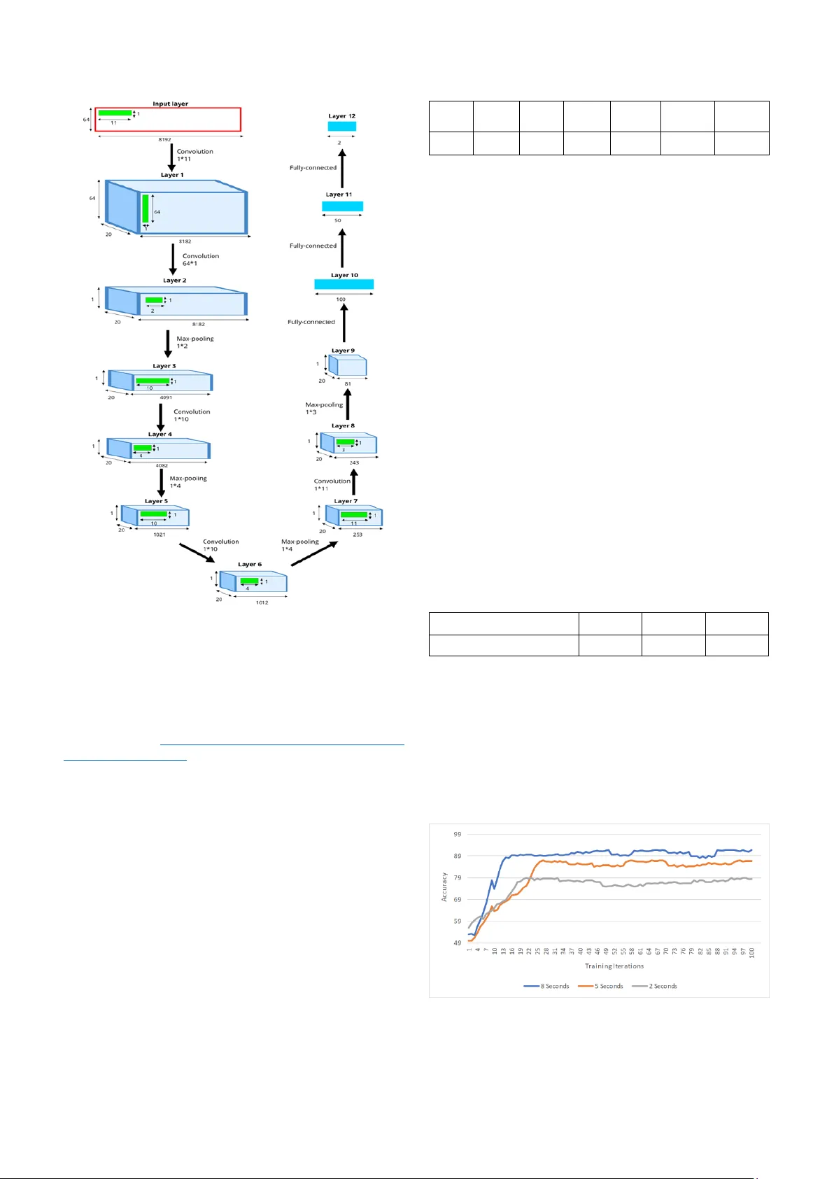
XXX -X-XXXX- XXXX -X/XX/$XX. 00 ©20XX I EEE Deep Convolutional Neural Network for Automated Detection of Mind W andering using EEG Signals Abstract — Mind wandering (MW) is a ubiquitous phenomenon which reflects a s hift in attention from task-r elated to task-unrelated thoughts. There is a need for intelligent interfaces that can reorient attention w hen MW is detected due to its detrimental effects on performance and productivity. In this paper, w e pr opose a de ep learning model fo r MW d etection using Electroencephalogram (EEG) signals. Specifically , w e develop a cha nnel-wise deep convolutional neural network (CNN) model to classify the features of focusing state a nd MW extracted from EEG signa ls. This is the first study that emp loys CNN to automatically detect MW using only EEG data . The experimental results on the collected dataset de monstra te promising performance with 91.78% accuracy, 92.84% sensitivity, and 90.73% specificity. Keywords — mind wandering, deep learning, c onvolutional neural network, electroencephalogram I. I NTRODUCTI ON Most people have had the experience of a shift in their focus from an attention-dem anding task at hand , such as reading books or driving , to task -unrel ated concerns. For instance, they may be thinking of events which happened in the past, may happen in the futu re, or never happen at all. This stimu lus-independent experie nce, wh ich is a series of imagin ative thought interm ittently during sustain ed attenti on task, is calle d mind wanderin g (MW) [1]. Although some research link ed MW to increa sed creativity [2], other studie s indicated that MW can lead to errors and a decrease in perform ance in various t asks [3]. Moreove r, there ar e evidences that support the correlation between MW and emotional disorders, such as neuroticism, alexithym ia, and dissociati on [4], [5 ] . Given the ubiquity an d negat ive consequenc es o f MW , it is beneficial to detect when MW occurs a nd then intervene to restore attenti on to the task at hand. As an initial step in this directi on, this paper proposes a n automated model to detect m omentary occurrenc es of MW. MW detection is a relat ively unex plored field. A majority of res earch have correlated oculom etr ic measu res such as blink rat e [6], pupil diameter and response , and eye gaze [ 7][8] to MW. Zerh o uni et al. [9] provide d an online measure o f MW using fMRI sam pling. Recent ly , there is a trend to study MW using EEG signals. Kawashim a et al. [10] utilized the combination o f EEG variables and non-linear regression modeling as an indic ator of MW . Qin e t al. [11] characte rized MW with an increase d gamma band activity in EEG sign als. Son et al. [12] showed an increase in frontal EEG theta/ beta ratio du ring MW . However, th e collecte d cognitiv e results by these techni ques are inconclu sive, disputable and sometim es contradi ctory [13][14]. That is why finding a data-driven technique that can detect MW accurat ely, effic iently is vital. Deep learning techniques have b een vastly used to perform tasks such as makin g predictions and decisions. Recently , researche rs have applied CNN, one type of deep learning models, on EEG signals. For instance, Schir rmeister et al. [15] studied a range of different CNN architectures for EEG decoding an d visualiz ation. Ha jinoroozi e t al. [16] design ed a CNN to predict driver fatig ue using 37 test partici pants’ EEG signals. A char ya et al. [17] utilized the CNN to diagnose epilepti c seizure using EEG signals. Since EEG sig nals are no nlinear and nonsta tionary in nature, we p ropose to employ CNN for the automatic identif ication o f MW only using raw EEG signals . To the best of our knowledge, this is the first study that employs CNN for autom atic detecti on o f MW based on EEG data. The order of content in this paper is as foll ows: section 2 d escrib es the datase t used in this study; section 3 explains the architectu re of the propos ed CNN , and training and testing process es; section 4 show s the performan ce based on experim ental resu lts; an d section 5 conclud es the p aper. II. DATASET PREPARATION A. S ubjects and proce dure EEG data used in th is research was acquire d by Grandcham p et al. at the Un iversity of Toulouse (Data is available on : https://sc cn.ucsd. edu/publi cly available EEG data.htm l ) [13]. Datasets were collecte d from two participants , a female age 25 and a male age 31 both without mental or neurologi cal disorder . Here w e summarized the data collecti on procedure. More details are available in the original paper [13] . Particip ants sat in a dimly lit room in front of a computer screen. The task of the participants w as to count backw ard each of their breath cycles (inhale/exhale ) from 10 to 1 repeate dly. The m ental sta te f or the backward count ing is referre d as focusing state (FS) . Participants had to press a mouse button when ever they realized they had lost track of their br eath coun t (i.e. MW h appens). Th ey then fill ed a short questionnai r e d escribin g their mind wandering episode and pressed a button to resume the task . Each parti cipant took ten 20 - mi n sessions perform ing the above p rocedu re. EEG data were captured using a 64 channel Biosem i Active Two system . The sampling rate was 1024 Hz . The data w as recorded continuous ly throug h the w hole session s . B. Train ing data selection There are two comm on strategies to define trainin g data and target labels: trial-w ise an d cropp ed train ing strategy [15] . Trial-w ise strategy considers th e entire trial as one input sample with multiple l abels, which indicat e the correspondin g events. Cropped-train ing strategy ext racts time w indows from a trial and assigns only o ne label for each time window. The assigned labels describe the event s happene d in th at time window . We use the cropped training strategy in this work. We extract ed MW episodes as positive samples and FS episodes as neg ative samples. Fig. 1 sh ows a h eatm ap of a 1 0- second interval o f one EEG data session . This time window contains 5 seconds before and after the button w as pressed . From Fig. 1, we can identify three distinc t time blocks : the Seyedroohollah Hosseini Department of Computer Science and Engineering University of North Texas Denton, Texas, USA sh0773@unt.edu Xuan Guo Department of Computer Science and Engineering University of North Texas Denton, Texas, USA xuan.guo@unt.edu first time block fr om the b eginn ing to the point w hen the partici pants realized MW, the second time block un til the button was press ed , and the l ast tim e bl ock th at the p articipant was answering the questionn aire. Fig. 1 clearly provides som e interesting pattern s of m ental states for FS and M W. Fig. 1. Heatmap of 10-second EEG da ta. There is a change in EEG data before the button press. We used MNE [18], an open-source python software, for training sam p le selection and data pre paration (Source code is available on: https://g ithub.c om/Biocom p uting-Resear ch- Group/MW-Data- Selecti on ). A to tal of 950 samples of 8 seconds were extracte d from the o rigin al EEG data, 475 FS and 475 MW sam p les . We tried multiple time window lengths, and 8 seconds gave the best pe rform ance. More details are in sect ion 4. T he FS samples are the time interval s that the p artici p ants keep track o f their breath counting . T he FS samples were randomly chosen from original data after th e breath coun ting starte d. Grandcham p et al [13] considered MW epis odes as a 10 -secon d inte rval prior t o the b utto n press ed . Howev er, Fig. 1 shows th at ther e is a clear chang e in the EEG signal before the button is pressed, which might be highly related to the mental activities resp onsible for re alizing the occurr ence of M W or hitti ng the button . Ou r observati ons show that this change lasts less than 2 sec onds. T heref ore, i n order t o have a cle an sam p le w ith only MW sign als , w e considere d an 8-second time win dow, sta rting 10 s econds before the button press. We also did a bandwidth filterin g of 0.5 – 50 Hz, given th e routine clinic al EEG ban dwidth is 0.5- 50 Hz [ 19]. T he extracted EEG samples were norm alized by Z-score norm alization w ith a zero mean and a stan dard deviation of 1. III. CNN MODEL A. A rchitechture For the data sample representa tio n, since EEG signals are the approxim ation of global voltage patterns from mu ltiple sources of the brain, we consider not to co mbin e these patterns, and use the whole set of electrodes. We also treat EEG as global m o dulati on in tim e and space. In this study, we used the representati on proposed by Schirrmeiste r et al. [15] which represents the input as a 2-D array wh ere channels (electr odes) are row s and amplitude (voltage ) across the time steps ar e colum ns. The aim of the model is to automatical ly and exp lici tly extract features which are u seful for EEG signal classificati on. Here, w e propose a generi c archite cture that can reach a competitiv e accu r acy . Our CNN has 12 layers including 4 convoluti on-max -pooling blocks, and t hree fully connected layers. Table 1 describes the details of the propos ed CNN structure . Table 1 . Deta ils of CNN struc ture used in this rese arch Layer s Type Kernel size Stride Output feature size 1 Convolution 1 × 11 1 64 × 8182 × 20 2 Convolution 64 × 1 1 1 × 8182 × 20 3 Max-pooling 1 × 2 2 1 × 4091 × 20 4 Convolution 1 × 10 1 1 × 4082 × 20 5 Max-pooling 1 × 4 4 1 × 1021 × 20 6 Convolution 1 × 10 1 1 × 1012 × 20 7 Max-pooling 1 × 4 4 1 × 253 × 20 8 Convolution 1 × 11 1 1 × 243 × 20 9 Max-pooling 1 × 3 3 1 × 81 × 20 10 Fully-connecte d - - 100 11 Fully-connecte d - - 50 12 Fully-connecte d - - 2 The first co nvolu tion layer receives input data. A k ernel of size 1 × 11 perform s a temporal convolution o ver time. It captures the correla tion among signal in each ch annel. I t outputs 20 s ets of f eatures. EEG sig nals produced b y the brain have spatial correlati o n, meani ng that all 64 channels capture the electrical activity of the brain wh ere m ultiple brain regions might w o rk togethe r. Therefore, the second layer takes a spatial filterin g with a kernel size of 64 × 1 to o btain the correlati on among channels . The kernel size and stride were chosen by the trial and error. Our experim ents show ed that the similar kernel size and str ide across these convolution layer s can achieve better classificati on accuracy (data not shown in this p aper ). T he r ectifi ed line ar unit (RELU) function w as used as activation function for each convolutiona l lay er . During the train ing, we u sed a dropout lay er w ith dropout rate 0.2 after the last max-poolin g layer. The used loss functi on is cross entropy function . Backpro pagation was p erform ed to calculat e gra dients (partial derivatives ) and update the paramete rs by A dam optim izer [20]. Classific ation block consists of thr ee fully-conn ected layers. The first fully-connect ed lay er gets the feature map output by the f orth feature extraction block. This lay er out p uts 100 fea tures. The second fully — conne cted layer generates 50 features. Finally, the third ful ly-connecte d layer p roduc es 2 features th at w ill be fed int o Softm ax function t o generat e the probability of each class label. Fig. 2 depicts the graphical represent ation of proposed CNN stru cture fo r MW detection . B. Train ing and testing Ten-fold cross validation [21] was used to test the generaliz ed performance of our CNN in classify ing MW and FS . We randomly divide d th e whole dat a t o ten equal portions (folds) . Eight o ut of ten folds were used to train the model, one of the last two fol ds was used for validati on, and the last one was utilized fo r t esting the model. We repeate d this procedu re ten times such tha t all folds were used to test th e model once. Each repetition o f ten-fold cross valid ation includes 100 epochs, meaning that the nu mber o f ite rations through the training set is 100 for backp ropagati o n. Fig. 2. The deep CNN architecture for MW dete ction IV. E XPERIMENT S AND RESULTS The proposed CNN m odel w as implemen ted on a workstation with I ntel Xeon 2.6 GHz (Silver 4112), 32 GB random access memory (RAM), and 8 GB DDR5 graphic card (NVidia Quadro P4000) with 1792 CUDA cores using P ython 3.6 and PyTorch machine learning library (Source code is available on: h ttps://g ithub.c om/Biocom puting-Research - Group/MW-Dete ction ). Seven metri cs were used t o m easure the performan ce: true positive, true negative, fa lse positive , false negative, accuracy, sensitivity , and specificity . Positive means MW is identifie d by model, and negative means the model rejects the happen ing of MW . True positiv e is the total num ber of times the model correctly identifies MW . True negative counts the total number of times the model correctly rejects MW . False positive is the number of times the model incorrectly identifies the occurrence of MW . False negative is the total number of times the model incorrectly rejects the happenin g of MW . Accuracy quantifi es the ability of model for the task of MW classifi cation by averaging the truly classified samples over the total. Sensitiv ity measu res the proportion of true positives . Specificity measures the pr oportion of true negativ es. Table 2 presents the confusion matrix of the model results for the MW classifi cation task . Table 2 . Overall classificatio n result across 10 fo lds True positive True negative False positive False negative Accuracy Sensitivity Specificity 441 431 34 44 91.78% 92.84% 90.73% A. P erformance compa rison of varied time window leng ths In order to decide the best time interva l o f a data sample , we tried three different lengths: 2, 5 , and 8 seconds. So, we obtained three trainning datasets. The sam e CNN m o del as i n section 3 were used with max-pooling la yers size modified . More specifically, all these CNN models have 4 max-pooling layers . T he m odel for 8-second data samples has the first max-pooling size set to 1 × 2 with stride 2, the s econd and the third layers set to 1 × 4 w it h stride 4, and the f orth layer set to 1 × 3 with stride 3. The CNN m odel for 5- second has the first and the s econd max-pooling la yers set to size 1 × 2 with s tride 2, the third la yer set to 1 × 3 with stride 3 , and the forth layer set to 1 × 4 with stride 4. T he model for 2-second data s amples has the first and second max-po oling la yers set to size 1 × 2 with stride 2 , the third layer set to 1 × 3 w ith stride 3, and the final max-pooling layer set to 1 × 2 with stride 2. The classificatio n results ar e shown in T able 3. T he results show t hat 8-second yield ed the best classification rate . The 8 -second gave the classificatio n accuracy of 91.78 %, while the classification r ate for 5 -second and 2-second are 86.63% and 78 .52% respectively. However, the ga in from changing 5-seco nd to 8-secon d is marginal co mpared to the one from changing 2 -second to 5-second. Table 3. Classificat ion accuracy for diffe rent sample lengths Sample le ngth (second) 2 5 8 Classification a ccuracy (%) 78.52 86.63 91.78 Fig. 3 sho ws the change of c lassification acc uracy over the number o f itrations for these datasets. Because the original p aper [13] defined MW as 10 -second time windows prior to the b utton press, and we excluded the 2-second ti me windows before the butto n press from o ur positive data samples d ue to the change i n EEG heatmap ( see Fig.1) , the extracted 8-second time windo ws are the longest time windows that can be used as MW samples in this work. Fig. 3. Classifica tion accuracy o f the selected sam ple length B. P erformance compa rison with ind ividual variation There was an interest to figu re out if different subjects might produ ce some patterns of MW specifi c to each sub ject . In other words, we want to test if there is any considerable feature-w ise difference between our male and female partici pants regarding the MW detecti on . To do so, we employ ed the propose d CNN model in th ree classifi cation runs. In the first run , we train ed the CNN only using the EEG data captured from the male participant and tested the model using the dat a belong s to the fem ale partici pant. In the second run, we did the training and testin g in an opposite way that u se the data f rom the female participant to t r ain the model an d test it u sing the data f rom the m ale participant . In the third run , we selected training and test samples randomly from the whole dataset including both m ale and fem ale. To maintain the same sizes for trainin g and testing, in these three runs, we divide d the wh ole dataset to three parts , the first part containin g 380 out of the 475 data samples (40% of wh ole d ataset) to train the CNN , the second part containin g 95 o ut of the 950 (10% of the wh ole dataset) for validati on, and the third part including 475 data s amples use d to test the model. The classifi cation results are show n in Tabl e 4. The m odel yield ed the classificati o n accuracies o f 67.63 % and 65.26 % for the first two r uns , respecti vely, and 81.84% classificatio n accuracy f or th e third ru n. The perform ance lapse between the first two runs an d th e las t r un supports th at th ere may be som e unique fea tures of MW o r FS to in dividuals . Further study on these featu res related to MW at ind ividual lev el are n ecessary which is beyond the scope of this work. Table 4 . Classifi cation result fo r the exper iment with gender fac tor Experiment run Accuracy First run 67.63% Second run 65.26% Third run 81.84% V. CONCLUSION In this work , the deep CNN model is employed for the first time to detect MW using only EEG data . One advant age of this model is that it d oes not need to hav e an explicit step to extract features, which is integr ated in the classification process . The model archite cture was chosen by the trial and error. We consi dered three time w indow len gths and found 8- second give the best performance. T he experimen t al results show ed that o ur model can achieve the classific ation accuracy up to 91.78%. The s ignificant d rop of cl assificati on r ates between each partici pant and the m ixed data demonstrated that there might be som e individual specific features of MW. For obtaining a good generalizati on performan ce, a diversi ty of data is required. The initial success of our model warrants our future study to apply the same deep learning a pproach on new datase ts for automated MW detection . REFERENCES [1] C. Braboszcz and A. Delo rme, “Lost in thoughts: Neural markers of low a lertness during mind wandering,” Neuroimage , vol. 54, no. 4, pp. 3040 – 3047, 2011. [2 ] G . A. Shaw and L. M. Giambra, “Task -unrelated thoughts of college stud ents diagnosed a s hyperactive i n chil d hood,” Dev. Neuropsychol. , vo l. 9, no. 1, pp. 17 – 30, 1 993. [3] J. C. Mcvay, M. J. Kane, and T . R. Kwapil, “T racking the train of thought from the laboratory into every day life: An experience- sampling study of mind w a ndering across controlle d and ecological contexts,” Psychon Bull Rev , vol. 16, no. 5, pp. 857 – 863, 2009. [4] S. G . Jensen, C. G ., Nicl asen, J., V angkilde, S. A., Peterse n, A., & Hasselba lch, “Ge neral inattentiveness is a long -term reliable trait independently p redictive of psychological health: Danish validation studies of the Mindful Attention Aw areness Scale,” vol . 28, no. 5, pp. 7 0 – 87, 2016. [5] R. A . B aer, G. T. Smith, J . Ho pkins, J. K rietemeyer, and L. Toney, “Using self -report assessment methods t o explore facets of mindfulness,” Assessm ent , vol. 13, no . 1, pp. 27 – 45, 200 6. [6] D. Smilek, J. S. A. Carriere, and J. A. C heyne , “Out of mind, out of sight: e ye blinking as indicator and embodiment of mind wandering.,” Psychol. Sci. a J. Am. Psychol. Soc. / APS , vol. 21, no. 6, pp. 786 – 789, 2010. [7] P. W. Kandoth and D. H. Deshpande, “Automatic gaze -based user- independent detection of mind wandering during compute rized reading,” J. Pos tgrad. Med. , vol. 16, no. 4, pp. 205 – 208, 19 70. [8] J. Smallw ood et al. , “P upillometric e vidence for the d ecoupling of attention from perceptual input during offline thought,” PL o S One , vol. 6, no. 3, 201 1. [9] E. A. Zerhouni and R. A. Collins, “Experience sampling du ring fMRI reveals default network and executive system contributions to mind wanderi ng,” Sci. Mag. , 2006. [10] I. Kawashima and H. Kumano, “Prediction of Mind -Wandering with Electroe ncephalogram an d Non-linear Regr ession Modeling,” Front. Hum. Neurosci. , vol. 11, no. July, pp. 1 – 10, 2017. [11] J. Qin, C. Perdoni, and B. He, “Dissociation of subjective ly reported and b ehavioral ly indexed mind wande ring by EEG rhythmic activ ity,” PLoS One , vol. 6, no. 9, 2011. [12] D. van Son, F. M. De Blasio, J. S. Fogarty, A. Angelidis, R. J. Barry, and P. Putman, “Frontal EEG theta/beta ratio during mind wandering episo des,” Biol. Psychol. , vol. 140, pp. 19 – 27, 2019. [13] R. Grandchamp, C. Br a boszcz, and A. Delorme, “Oculometric variations during mind wandering,” Front. Ps y chol. , v ol. 5, pp. 1 – 10, 2014. [14] R. Grandchamp et al. , “Pupil dilation during mind wander ing,” vol. 9, no. 3, p. 1 8298, 2011. [15] R. T. Schirrmeister et al. , “Deep learning with convolutional neural networks for EEG deco ding and vis ualization,” Hum. Brain Mapp. , vol. 38, no. 11, pp. 5391 – 5420, 2 017. [16] M. Hajinoro ozi, Z. Mao, T. P. Jung, C. T. Lin, and Y. Huang, “EEG - based prediction of drive r’s cognitive per formance by dee p convolutional neural networ k,” Signal Process. Image Co mm un. , vol. 47, pp. 549 – 555, 2016. [17] U. R. Acharya, S. L . Oh, Y. Hagiwara, J. H. Tan, and H. Adeli, “Deep convolutional neura l network for the automated detection and diagnosis of seizure using EEG signals,” Comput. Biol. Med. , vol. 100, pp. 270 – 278, 2018. [18] A. Gramfo rt et al . , “MNE softw are for processing MEG an d EEG data,” Neuroimage , vol. 86, pp. 44 6 – 460, 2014. [19] S. Van hatalo, J. Voipio, and K. Kaila, “Full -band EEG (FbEEG): An emerging standard in electroencephalogr aphy,” Clin. Neurophysiol. , vo l. 116, no. 1, pp. 1 – 8, 2005. [20] D. P. Kingma and J. Lie Ba, “A DAM: A Method for Stochast ic Optimization,” I CLR , vol. 1631, pp. 5 8 – 62, 2015. [21] R. O. Duda, P. E. Hart , and D. G. Stork, Patter n C lassification 2nd Edition . 2001.