Methods of interpreting error estimates for grayscale image reconstructions

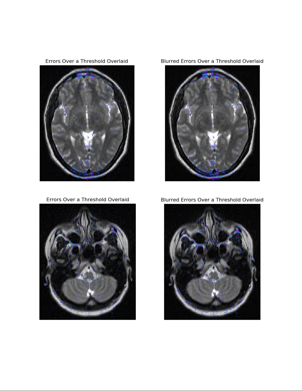
Metho ds of in terpreting error estimates for gra yscale image reconstructions Aaron Defazio and Mark T ygert F ebruary 5, 2019 Abstract One represen tation of p ossible errors in a gra yscale image reconstruction is as another gra yscale image estimating p oten tially w orrisome differences b et ween the reconstruction and the actual “ground-truth” realit y . Visualizations and summary statistics can aid in the in terpretation of such a representation of error estimates. Visualizations include suitable colorizations of the reconstruction, as well as the ob vious “correction” of the reconstruction b y subtracting off the error estimates. The canonical summary statistic w ould b e the root-mean-square of the error estimates. Numerical examples inv olving cranial magnetic- resonance imaging clarify the relativ e merits of the v arious methods in the con text of compressed sensing. Unfortunately , the colorizations app ear lik ely to b e to o distracting for actual clinical practice, and the ro ot-mean-square gets sw amped by bac kground noise in the error estimates. F ortunately , straigh tforward displa ys of the error estimates and of the “corrected” reconstruction are illuminating, and the root-mean- square impro ves greatly after mild blurring of the error estimates; the blurring is barely perceptible to the h uman ey e yet smo oths aw ay bac kground noise that would otherwise ov erwhelm the ro ot-mean-square. 1 In tro duction Compressed sensing in imaging is a paradigm for accelerating the acquisition of full images by taking fewer measuremen ts than the num b er of degrees of freedom b eing reconstructed. The measurements are th us “undersampled” relativ e to the usual information-theoretic requiremen ts of sampling at the Nyquist rate etc. Compressed sensing therefore risks introducing errors, errors whic h v ery w ell ma y v ary among different image acquisitions. Recent work of [Tygert et al., 2018] and others generates an error “bar” for eac h reconstructed image, in the form of another image that can b e exp ected to b e representativ e of p otential differences b et w een the reconstruction and the real ground-truth. The present pap er considers user-friendly metho ds for generating visualizations and automatic interpretations of these error estimates, appropriate for display to medical professionals (esp ecially radiologists) on data of cranial scans from magnetic-resonance imaging (MRI) mac hines. After testing sev eral natural visual displays, w e find that an y nontrivial visualization is likely to b e to o distracting for physicians, as some hav e expressed reserv ations ab out ha ving to lo ok at any errors at all — they would b e muc h happier having a machine lo ok at the estimates and flag p oten tially serious errors for sp ecial consideration. W e migh t conclude that colorization is to o distracting, that the b est visualizations are simple displays of the error estimates, p ossibly supplemented with the error estimates subtracted from the reconstructions (th us sho wing ho w the error estimates can “correct” the reconstructions). Most of the results of the presen t pap er ab out visualization could be regarded as negative, how ev er natural and straightforw ard the colorizations ma y b e. F or circumstances in which visualizing errors is ov erkill (or unnecessarily b othersome), we find that an almost simplistic automated interpretation of the plots of errors — rep orting just the ro ot-mean-square of the denoised error estimates — w orks remark ably well. While background noise dominates the ro ot-mean-square of the initial, noisy error estimates, even denoising that is almost imp erceptible can remov e the obfuscatory bac kground noise; the ro ot-mean-square can then fo cus on the remaining errors, which are often relatively sparsely distributed. When the root-mean-square of the denoised error estimates is large enough, a clinician could look at the visualizations mentioned ab o ve to fully understand the implications of the error estimates (or rescan the patien t using a less error-prone sampling pattern). 1 2 Metho ds 2.1 Visualization in gra yscale and in color W e include four kinds of plots displa ying the full reconstructions and errors: 1. “Original” is the original gra yscale image. 2. “Reconstruction” is the reconstruction via compressed sensing. Sp ecifically , we use the configuration of [Tygert et al., 2018]; for details (which are largely irrelev an t for comparing the utility of visualiza- tions), please see the third section, “Numerical examples,” of [T ygert et al., 2018]. 3. “Error of Reconstruction” displa ys the difference b et w een the original and reconstructed images, with blac k (or white) corresponding to extreme errors, and middling grays corresponding to the absence of errors. 4. “Bootstrap” displays the errors estimated via the b o otstrap of [Tygert et al., 2018] (using the same 1000 iterations used by [T ygert et al., 2018]), with black (or white) corresp onding to extreme errors, and middling gra ys corresp onding to the absence of errors. W e visualize the errors in reconstruction and the b o otstrap estimates using gra yscale so that the phases of oscillatory artifacts are less apparent; colorized errors lo ok very different for damp ed sine versus cosine w av es, whereas the medical meaning of such wa v es is often similar. App endix A displa ys the errors in color. W e consider four metho ds for visualizing the effects of errors (as estimated via the b ootstrap) sim ultane- ously with displaying the reconstruction, via manipulation of the hue-saturation-v alue color space describ ed, for example, b y [v an der W alt et al., 2014]: 1. “Reconstruction - Bo otstrap” is literally the b o otstrap error estimate subtracted from the reconstruc- tion, in some sense “correcting” or “enhancing” the reconstruction. 2. “Errors Over a Threshold Overlaid” iden tifies the pixels in the bo otstrap error estimate whose absolute v alues are in the upp er p ercen tiles (the upp er tw o p ercen tiles for horizontally retained sampling, the upp er one for radially retained sampling), then replaces those pixels (retaining all other pixels un- c hanged) in the reconstruction with colors corresp onding to the v alues of the pixels in the b ootstrap. Sp ecifically , the colors plotted are at the highest v alue p ossible and fully saturated, with a hue ranging from cyan to magenta, with blue in the middle (how ever, as we include only the upp er p ercen tiles, only hues very close to cyan or to magen ta actually get plotted). This effectively marks the pixels corresp onding to the largest estimated errors with eye-popping colors, leaving the other pixels at their gra y v alues in the reconstruction. 3. “Bootstrap-Saturated Reconstruction” sets the saturation of a pixel in the reconstruction to the cor- resp onding absolute v alue of the pixel in the b o otstrap error estimate (normalized by the greatest absolute v alue of an y pixel in the b o otstrap), with a hue set to red or green dep ending on the sign of the pixel in the b ootstrap. The v alue of the pixel in the reconstruction stays the same. Thus, a pixel gets colored more intensely red or more intensely green when the absolute v alue of the pixel in the b ootstrap is large, but alwa ys with the v alue in hue-saturation-v alue remaining the same as in the original reconstruction; a pixel whose corresp onding absolute v alue in the b ootstrap is relatively negligible sta ys unsaturated gra y at the v alue in the reconstruction. 4. “Bootstrap-Interpolated Reconstruction” leav es the v alue of each pixel at its v alue in the reconstruc- tion, and linearly interpolates in the hue-saturation plane b etw een green and magenta based on the corresp onding v alue of the pixel in the b ootstrap error estimate (normalized by the greatest absolute v alue of any pixel in the b o otstrap). Pure gray is in the middle of the line b et ween green and magenta, so that an y pixel whose corresp onding error estimate is zero will app ear unc hanged, exactly as it was in the original reconstruction; pixels whose corresp onding error estimates are the largest hav e the same v alue as in the reconstruction but get colored magenta, while those whose corresponding error estimates are the most negativ e ha ve the same v alue as in the reconstruction but get colored green. 2 2.2 Summarization in a scalar The square ro ot of the sum of the squares of slightly denoised error estimations summarizes in a single scalar the o verall size of errors. Ev en inconspicuous denoising can greatly improv e the ro ot-mean-square: While the effect of blurring the b ootstrap error estimates with a normalized Gaussian conv olutional k ernel of standard deviation one pixel is almost imp erceptible to the h uman eye (or at least preserv es the semantically meaningful structures in the images), the blur helps remov e the background of noise that can otherwise dominate the ro ot-mean-square of the error estimates. The blur largely preserves significant edges and textured areas, y et can eliminate m uch of the perceptually immaterial zero-mean background noise. Whereas bac kground noise can o verwhelm the root-mean-square of the initial, noisy b ootstrap, the ro ot-mean-square of the sligh tly blurred bo otstrap captures the magnitude of the imp ortan t features in the error estimates. 3 Results Our data comes from [Loizou et al., 2013a], [Loizou et al., 2011], [Loizou et al., 2013b], [Loizou et al., 2015]. Sp ecifically , w e consider tw o cross-sectional slices through the head of a patien t in an MRI scanner: the lo wer slice is the third of tw en ty from [Tygert et al., 2018], while the upp er slice is the tenth of tw en ty from [Tygert et al., 2018]. Compressed sensing reconstructs a cross-sectional image given only a subset of the usual measurements of v alues of the tw o-dimensional F ourier transform of the original, “ground-truth” cross-section. W e consider the radially retained and horizon tally retained subsets of [Tygert et al., 2018], whic h yield the error estimates display ed in the figures b elo w (the third section, “Numerical examples,” of [Tygert et al., 2018] details the sch emes for sampling, but these details are irrelev ant for assessment of visualizations). W e used the Python pack age (“fb oo ja”) of [Tygert et al., 2018]; the Gaussian blur from Subsection 2.2 lev erages skimage.filters.gaussian from scikit-image of [v an der W alt et al., 2014]. Figures 1–8 display the visualizations from Subsection 2.1. Figures 9 and 10 depict the effects of the Gaussian blur from Subsection 2.2. T able 1 rep orts how drastically such a nearly imp erceptible blur changes the square roots of the sums of the squares of the error estimates. Background noise clearly ov erwhelms the ro ot-mean-square without an y denoising of the error estimates — the ro ot-mean-square decreases dramati- cally ev en with just the mild denoising of blurring with a normalized Gaussian conv olutional kernel whose standard deviation is one pixel, as in T able 1 and Figures 9 and 10. T ables 2 and 3 report how blurring with wider Gaussians affects the ro ot-mean-square; of course, wider Gaussian blurs are muc h more conspicuous and risk washing out imp ortant coheren t features of the error estimates, while the last column of T able 3 sho ws that denoising with wider Gaussian blurs brings diminishing returns. The width used in T able 1 and Figures 9 and 10 — only one pixel — ma y b e safest. Appendix B displays the grayscale reconstruc- tions ov erlaid with the blurred bo otstraps (blurring with a Gaussian whose standard deviation is one pixel), thresholded and colorized as in Subsection 2.1. 4 Discussion and Conclusion Broadly sp eaking, the b ootstrap-saturated reconstructions and b ootstrap-interpolated reconstructions lo ok similar, ev en though the details of their constructions differ. Both the b ootstrap-saturated reconstruction and the bo otstrap-in terp olated reconstruction highligh t errors more starkly on pixels for whic h the reconstruction is brigh t; dark green, dark red, and dark magen ta (that is, with a relatively lo w v alue in hue-saturation-v alue) simply do not jump out visually , ev en if the green, red, or magen ta are fully saturated. That said, retaining the v alue of the pixel in the reconstruction mak es the colorization of the bo otstrap-saturated reconstruction and the b ootstrap-interpolated reconstruction far less distracting than in errors ov er a threshold ov erlaid, with muc h higher fidelit y to the form of the grayscale reconstruction in the colored regions. Of course, the errors o ver a threshold o v erlaid do not alter the grayscale reconstruction at all when the errors are within the threshold, so the fidelit y to the gra yscale reconstruction is perfect in those areas of the image s with o verlaid errors where the error estimates do not go b ey ond the threshold. Th us, none of the colorizations is uniformly sup erior to the others, and all may b e to o distracting for actual clinical practice. Alternativ es include direct displa y of the b ootstrap error estimates, p ossibly 3 T able 1: square ro ots of the sums of the squares of the error estimates Sampling Slice Bo otstrap Blurred Bootstrap horizon tally lo wer 12.9 6.25 horizon tally upp er 13.8 7.34 radially lo wer 17.5 10.5 radially upp er 18.0 11.6 T able 2: square ro ots of the sums of the squares of the error estimates for the low er slice blurred against a Gaussian conv olutional kernel of the sp ecified standard deviation (the standard deviation is in pixels), for sampling retained horizon tally or radially Std. Dev. Horizontally Radially 0.0 12.9 17.5 0.5 9.94 14.6 1.0 6.25 10.5 1.5 4.38 8.06 2.0 3.03 6.34 2.5 2.04 5.06 3.0 1.33 4.09 3.5 .847 3.34 4.0 .535 2.75 complemen ted by the bo otstrap subtracted from the reconstruction (to illustrate the effects of “correcting” the reconstruction with the error estimates), which are readily interpretable and minimally distracting. The b ootstrap subtracted from the reconstruction tends to sharp en the reconstruction and to add bac k some features suc h as lines or textures that the reconstruction obscured. How ever, this reconstruction that is “corrected” with the bo otstrap estimations may con tain artifacts not present in the original image — the error estimates tend to b e conserv ative, p ossibly suspecting errors in some regions where in fact the reconstruction is accurate. The “corrected” reconstruction (that is, the bo otstrap subtracted from the reconstruction) can b e illuminating, but only as a complemen t to plotting the bo otstrap error estimates on their own, too. A sensible proto col could b e to chec k if the ro ot-mean-square of the blurred b ootstrap is large enough to merit further inv estigation, in v estigating further by lo oking at the full b ootstrap image together with the reconstruction “corrected” b y subtracting off the bo otstrap error estimates (or colorizations). T able 3: square ro ots of the sums of the squares of the error estimates for the upper slice blurred against a Gaussian conv olutional kernel of the sp ecified standard deviation (the standard deviation is in pixels), for sampling retained horizon tally or radially Std. Dev. Horizontally Radially 0.0 13.8 18.0 0.5 10.9 15.3 1.0 7.34 11.6 1.5 5.35 9.50 2.0 3.82 7.97 2.5 2.63 6.79 3.0 1.75 5.87 3.5 1.14 5.13 4.0 .745 4.54 4 Figure 1: horizontally retained sampling — low er slice (a) 5 Figure 2: horizontally retained sampling — low er slice (b) 6 Figure 3: horizontally retained sampling — upp er slice (a) 7 Figure 4: horizontally retained sampling — upp er slice (b) 8 Figure 5: radially retained sampling — lo wer slice (a) 9 Figure 6: radially retained sampling — lo wer slice (b) 10 Figure 7: radially retained sampling — upper slice (a) 11 Figure 8: radially retained sampling — uppe r slice (b) 12 Figure 9: horizon tally retained sampling — upp er plots display the upp er slice; lo w er plots displa y the lo wer 13 Figure 10: radially retained sampling — upp er plots display the upp er slice; lo wer plots display the lo wer 14 A Bo otstraps and Errors in Color F or reference, this app endix displa ys the errors of reconstruction and b o otstrap estimates in color, with blue for negative errors, red for p ositiv e errors, and white for the absence of an y error (ligh t blue and light red indicate less extreme errors than pure blue or pure red). The lab eling conv en tions (“lo wer,” “upp er,” etc.) conform to those in tro duced in Section 3. 15 Figure 11: horizontally retained sampling — low er slice (c) 16 Figure 12: horizontally retained sampling — upp er slice (c) 17 Figure 13: radially retained sampling — lo wer slice (c) 18 Figure 14: radially retained sampling — upper slice (c) 19 B Blurred Errors Ov er a Threshold Ov erlaid F or reference, this appendix displays the same errors o v er a threshold o verlaid ov er the reconstruction as in Subsection 2.1, together with the blurred errors ov er a threshold ov erlaid ov er the reconstruction (blurring with a Gaussian conv olutional kernel whose standard deviation is one pixel, as in Subsection 2.2). The lab eling con ven tions (“low er,” “upp er,” etc.) conform to those introduced in Section 3. The blurred errors certainly introduce less distracting noise than without blurring, y et the colors still app ear really distracting. 20 Figure 15: horizontally retained sampling (b) — upper plots show the upper slice; low er plots show the lo wer 21 Figure 16: radially retained sampling (b) — upp er plots displa y the upp er slice; low er plots display the lo wer 22 References [Loizou et al., 2013a] Loizou, C. P ., Kyriacou, E. C., Seimenis, I., Pan tziaris, M., Petroudi, S., Karaolis, M., and Pattic his, C. (2013a). Brain white matter lesion classification in multiple sclerosis sub jects for the prognosis of future disabilit y . Intel. De cision T e ch. J. , 7:3–10. [Loizou et al., 2011] Loizou, C. P ., Murray , V., P attic his, M., Seimenis, I., P antziaris, M., and Pattic his, C. (2011). Multi-scale amplitude-mo dulation–frequency-mo dulation (AM-FM) texture analysis of multiple sclerosis in brain MRI images. IEEE T r ans. Inform. T e ch. Biome d. , 15(1):119–129. [Loizou et al., 2013b] Loizou, C. P ., Pan tziaris, M., Pattic his, C. S., and Seimenis, I. (2013b). Brain MRI image normalization in texture analysis of multiple scleros is. J. Biome d. Gr aph. Comput. , 3(1):20–34. [Loizou et al., 2015] Loizou, C. P ., Petroudi, S., Seimenis, I., Pan tziaris, M., and Pattic his, C. (2015). Quan- titativ e texture analysis of brain white matter lesions deriv ed from T2-w eighted MR images in MS patients with clinically isolated syndrome. J. Neur or adiol. , 42(2):99–114. [T ygert et al., 2018] T ygert, M., W ard, R., and Zb on tar, J. (2018). Compressed sensing with a jackknife and a bo otstrap. T echnical Report 1809.06959, arXiv. [v an der W alt et al., 2014] v an der W alt, S., Sch¨ on b erger, J. L., Nunez-Iglesias, J., Boulogne, F., W arner, J. D., Y ager, N., Gouillart, E., and Y u, T. (2014). Scikit-image: image pro cessing in Python. Pe erJ , 2(e453):1–18. 23