Designing nearly tight window for improving time-frequency masking

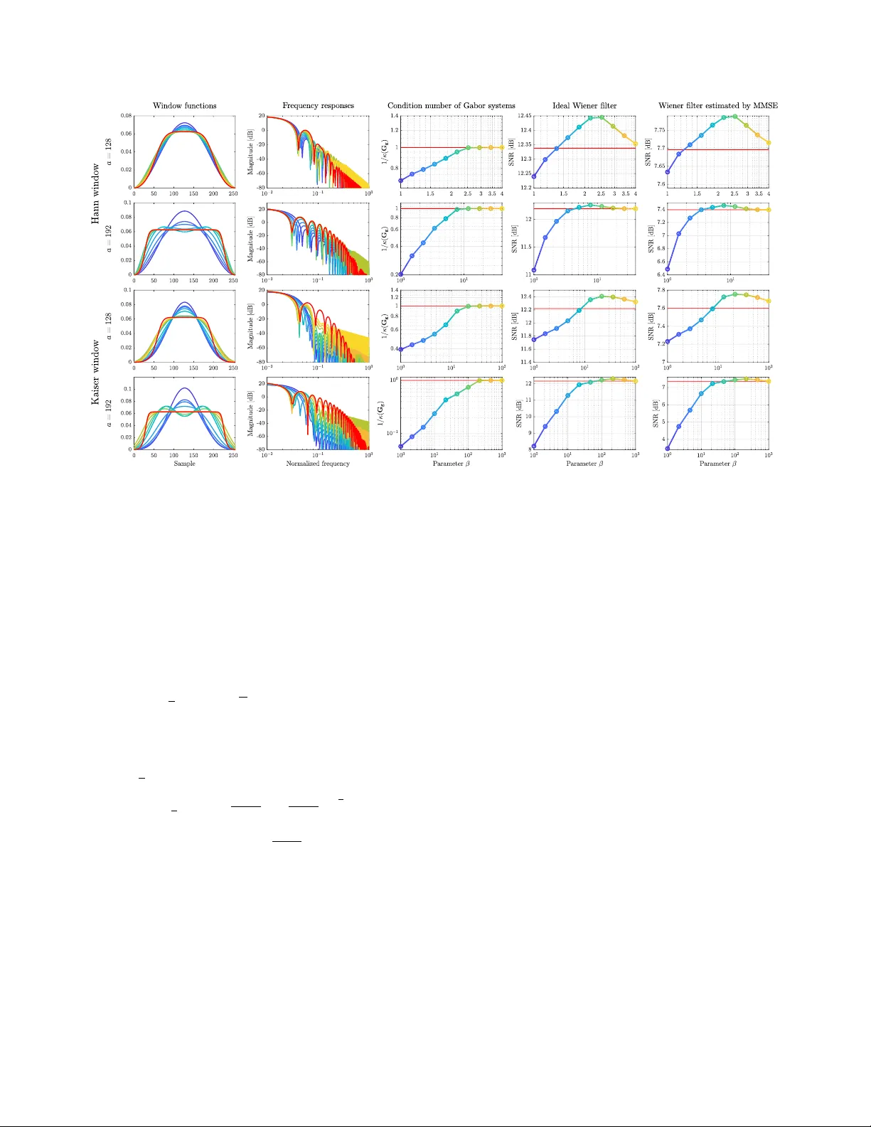
DESIGNING NEARL Y TIGHT WINDO W FOR IMPR O VING TIME-FREQUENCY MASKING Tsubasa K usano, Y oshiki Masuyama, K ohei Y atabe and Y asuhir o Oikawa Department of Intermedia Art and Science, W aseda Univ ersity , T ok yo, Japan ABSTRA CT Many audio signal processing methods are formulated in the time- frequency (T -F) domain which is obtained by the short-time Fourier transform (STFT). The properties of the STFT are fully character- ized by window function, number of frequency channels, and time- shift. Thus, designing a better window is important for improving the performance of the processing especially when a less redundant T -F representation is desirable. While many window functions have been proposed in the literature, the y are designed to hav e a good fre- quency response for analysis, which may not perform well in terms of signal processing. The window design must take the ef fect of the reconstruction (from the T -F domain into the time domain) into ac- count for impro ving the performance. In this paper , an optimization- based design method of a nearly tight windo w is proposed to obtain a window performing well for the T -F domain signal processing. Index T erms — Discrete Gabor transform (DGT), short-time Fourier transform (STFT), window design, speech enhancement, non-con vex optimization. 1. INTR ODUCTION Many audio signal processing methods are formulated as modifica- tions of the signal in the time-frequency (T -F) domain, which is often called T -F masking. For con verting the signal into the T -F domain, the short-time F ourier transform (STFT) [1] 1 is usually utilized o w- ing to its simplicity and easily understandable structure [2–8]. While most of the research has concentrated on the method of modification in the T -F domain (the way how to construct a T -F mask), the method of con verting a signal into the T -F domain is also important for im- proving the performance of processing. When STFT is considered as the con version to the T -F domain, its property is fully characterized by the window function since STFT is a highly structured transform. Aiming to obtain a better T -F representation, many window functions have been proposed to improv e their frequency responses [9–15]. For example, the Hann window is one popular window which has a good sidelobe decay . The Nuttall window was proposed to achieve a better sidelobe de- cay , while the Kaiser window was proposed so that its frequency response was adjustable by a tuning parameter . Although such re- search on window functions has provided a better T -F representation, most research only has considered the analysis side. That is, there is little research on window functions considering the r econstruction point of view . T o realize processing in the T -F domain, the signal must be re- constructed back into the time domain after the T -F-domain process- ing. The reconstruction side of STFT is achieved by the (pseudo-) 1 STFT is also often called the Gabor transform based on [1]. Note that some literature strictly distinguishes STFT from the Gabor transform by their mapping properties [2], while others do not. In this paper , we may utilize the term “STFT” in the sense of the discrete Gabor transform (DGT), which is a common habit especially in the acoustical signal processing community . in verse STFT which also in volv es a windo w function. Therefore, for the T -F domain signal processing, a window function must be cho- sen in accordance with not only STFT but also the inv erse STFT . Indeed, incorrect choice of the pair of window functions (for STFT and the in verse STFT) makes reconstruction impossible. T o allow a reasonable window for the reconstruction, the T -F representation is usually chosen to be r edundant , and the error-minimizing windo w called the canonical dual window is often used for the reconstruction (see Section 2). For some applications fav oring less redundant T -F representa- tion, choice of the window function is more critical for the recon- struction (and thus, critical for processing). One example is T -F masking in low-po wer devices which allow a little computation [16, 17]. In such cases, redundancy should be lowered because higher redundancy directly results in higher computational cost. Another very important example is speech enhancement based on deep learn- ing. Recent study has shown that non-redundant T -F representation can impro ve the performance of enhancement using deep neural net- works (DNN) [18]. This is because less redundant T -F representation reduces the number of parameters to be learned, which makes the training easier . For those applications, redundancy of STFT should be lowered by increasing the window shifting width. Howe ver , the in verse transform becomes more sensitiv e to the error of signal pro- cessing when the redundancy is reduced (see Section 2.3), which also degrades the performance. Although there exists a type of win- dow insensiti ve to such processing error, called tight window , it has a drawback that its frequency response is often poor (sidelobe lev el is high). Therefore, a window function which is less sensiti ve to pro- cessing error and, at the same time, has a good frequency response is desired for realizing a better processing in a less redundant situation. In this paper, we propose a window design method to simulta- neously meet both requirements. It aims to mak e a windo w function closer to a tight windo w , while its frequency response is constrained to be better . Since the designed window is not strictly tight, we call it nearly tight windo w . The proposed method is formulated as an op- timization problem so that it can easily control the trade-of f between the two requirements, and it is solved by the linearized alternating direction method of multipliers (ADMM). 2. PRELIMINARIES While the discrete and downsampled T -F transform is called “STFT” in acoustical signal processing, the literature of T -F analysis calls it the discrete Gabor transform (DGT) [2]. Hereafter, we will utilize the language used in DGT to e xpress the T -F representation because it will be easier for explaining the proposed method. 2.1. Gabor system and discrete Gabor transf orm (DGT) Let a windo w be denoted by g = [ g [0] , g [1] , . . . , g [ L − 1]] T ∈ R L . DGT is a T -F transform based on a collection of windowed sinusoids, G ( g , a, M ) = { g m,n } m =0 ,...,M − 1 , n =0 ,...,N − 1 , (1) which is called the Gabor system, where a ∈ N is the time-shifting width, M ∈ N is the number of frequency channels, g m,n [ l ] = e i 2 πml M g [ l − an ] , (2) is a windowed complex sinusoid, and i = √ − 1 . DGT of a discrete signal f ∈ R L is defined by the following inner product: ( G g f )[ m + nM ] = h f , g m,n i = L − 1 X l =0 f [ l ] g m,n [ l ] . (3) where x is the complex conjugate of x , and G g ∈ C M N × L is the matrix consisting of all the elements in the Gabor system in Eq. (1). That is, multiplying G g to a signal obtains the vectorized v ersion of its T -F representation which is often called “spectrogram. ” 2.2. Reconstruction of time-domain signal from T -F domain A system G ( g , a, M ) is said to be a frame [19, 20] if there exist 0 < A, B < ∞ such that A k f k 2 2 ≤ X m,n |h f , g m,n i| 2 ≤ B k f k 2 2 , (4) for all f ∈ R L , where k · k p is the ` p norm. A and B are called the lower and upper frame bound, respectiv ely . If the Gabor system is a frame, a time-domain signal can be reconstructed from its T -F do- main representation. The inv erse DGT , reconstructing a signal from its coefficients c ∈ C M N , with respect to G ( g , a, M ) is defined by f syn = X n,m c [ m + nM ] g m,n = G ∗ g c , (5) where G ∗ g denotes the comple x-conjugate transpose of G g . If a Ga- bor system G ( g , a, M ) is a frame, then there exists the correspond- ing dual Gabor frame G ( h , a, M ) = { h m,n } which satisfies f = X n,m h f , g m,n i h m,n , (6) where h m,n [ l ] = e i 2 πml M h [ l − an ] , and h is a dual window of g . That is, a time-domain signal can be reconstructed if (1) G ( g , a, M ) is a frame, and (2) h is a dual window of g . These conditions are decided by the window pair g , h , the time-shifting width a , and the number of frequency channels M . When a Gabor system G ( g , a, M ) is redundant, the correspond- ing dual window h is not unique, and infinitely many variation of h can satisfy the reconstruction formula, Eq. (6). One standard choice among all possible dual windows is the canonical dual windo w ˜ g = S − 1 g g , (7) where S g = G ∗ g G g is the so-called frame operator defined as S g f = X m,n h f , g m,n i g m,n = ( G ∗ g G g ) f . (8) The canonical dual window is optimal in the sense that its synthesis operator corresponds to the Moore–Penrose pseudo-in verse: X n,m c [ m + nM ] ˜ g m,n = X n,m c [ m + nM ] S − 1 g g m,n = ( G ∗ g G g ) − 1 G ∗ g c . (9) In this paper , the canonical dual window is considered for inv erse DGT as it is the standard choice in acoustical signal processing. One reason for such popularity should be because of the optimality to the following least squares signal reconstruction problem: minimize x k G g x − ˆ c k 2 2 , (10) whose solution is G ∗ ˜ g ˆ c as can be confirmed from the fact in Eq. (9). Modification of Gabor coefficients Inverse DGT DGT Input signal Gabor coefficients (Spectrogram) Modified coefficients Modified signal Fig. 1 . Framework of the signal processing in the T -F domain. Fig. 2 . (left) Condition number of the DGT matrix κ ( G g ) . (cen- ter) Denoising result using the ideal Wiener filter . (right) Denoising result using the W iener filter with MMSE noise power estimation. 2.3. Influence of window functions on signal pr ocessing A signal processing frame work in T -F domain is illustrated in Fig 1. In words, some processing is performed in the T -F domain to modify the Gabor coefficient c to ˆ c , and then the inv erse DGT is applied to obtain the processed result ˆ f . While the quality of the processing is important for obtaining a good result, the transformation pair, DGT and in verse DGT , is also important since it decides the coefficient c . T o see the effect of the window pair in terms of T -F domain signal processing, a preliminary experiment was performed. 200 speech signals [21] from TIMIT database [22] were degraded by adding the Gaussian noise in the time domain so that the signal-to- noise ratio (SNR) became 0 dB. They were enhanced by the Wiener filter (T -F masking based on the power ratio of noisy and clean sig- nals) with a minimum mean-square error (MMSE) estimator of noise power [8] and the decision-directed approach [6]. The redundancy was changed by changing a while fixing the window length to 256 and M = 256 . Its performance was compared with the ideal W iener filter and the condition number of G g , κ ( G g ) = σ max ( G g ) / σ min ( G g ) = p B / A , (11) which is the standard measure of numerical stability of Eq. (9), where σ max ( G g ) and σ min ( G g ) denote the maximum and mini- mum singular value of G g , respectiv ely . Three types of window functions were utilized for comparison: the Hann window , the Kaiser window ( α = 10) , and the canonical tight window of the Kaiser window . A window g T is said to be tight if its canonical dual window is itself (i.e., self-dual) [23]. Then, S = G ∗ g T G g T = A I (12) holds, where I is the identity . Thus, the condition number of a tight window is always 1. Particularly , a tight windo w with A = 1 is called the Parse val tight window . The canonical tight window of a window g can be obtained by inv erting square root of the frame operator: g T = S − 1 2 g g , (13) which corresponds to the solution of the following problem [24]: minimize x ∈T k g − x k 2 , (14) where T is the set of all P arseval tight windows. Thus, the canonical tight window is the closest Parsev al tight window from the window g . An efficient algorithm for its computation is available in the L T - F A T toolbox [25], see also [24]. Results of the experiment are shown in Fig. 2, where SNR is the av erage among all speech signals. For both ideal and realis- tic W iener filters (center and right), the processing performances of the Hann and Kaiser windows were degraded as the redundancy de- creased (horizontal axes are related to the redundancy). In contrast, the performance of the tight Kaiser windo w was not de graded much. These results can be predicted from the condition numbers (left). Based on this experiment, a window g should be designed so that the condition number κ ( G g ) becomes lower . A tight window is the best window in this sense because its condition number is the low- est. Howe ver , as in the figure, a tight window is not always the best in terms of processing, which is because the frequency response of a tight window is usually not better than one of a non-tight window (see Fig. 3). Therefore, in this paper , a design method of a nearly tight window is proposed so that the condition number is lowered while its frequency response is kept well. 2.4. Related works on Gabor window design For designing a low-condition-numbered window , design methods of tight windows have been proposed [26, 27]. These methods aim to find a tight window with better frequenc y responses. Howe ver , since the constraint to the tight window greatly limits the set of variables, desired characteristics may not be obtained. On the other hand, some methods of nearly-tight window de- sign have been proposed [28–30]. One approach of this research is to minimize the difference between the frame operator and iden- tity operator using the gradient-based optimization [28, 29]. These methods minimize the distance to the set of tight windows by the gradient method, whereby they have a possibility of falling into the local minima. Another approach is to replace the non-conv ex cost of measuring the distance to the tight windo w with con ve x func- tions [30]. Since that method is formulated as conv ex optimization, it is guaranteed that globally optimal solutions can be obtained, so a trade-off between the condition number and the frequency response can be easily considered. Howe ver , as a result of approximating the cost function, the obtained solutions may not be close to the original solution which is tight. The cost should be reduced strictly without approximation, while the trade-off should be easily adjusted. 3. PR OPOSED METHOD In this section, we propose a design method of nearly tight win- dow that can easily control the trade-off between the desired fre- quency response and the condition number . At first, we formulate the nearly tight Gabor window design as a constrained minimiza- tion problem. Then, an algorithm solving this problem through the proximal operators is introduced. Since a window whose support is shorter than the signal length is used in most signal processing, the formulation considers g [ l ] = 0 for l = K, . . . , L − 1 , i.e., only g [ l ] ( l = 0 , . . . , K − 1) are treated as the variables in this paper . 3.1. Problem f ormulation for designing nearly tight window T o propose an easily adjustable windo w function design, the desired frequency response is considered as a constraint, and the window is made closer to a tight window as possible. Its direct formulation is minimize g ∈C 1 2 d 2 T ( g ) , (15) where d T ( g ) is the distance to the set of Parsev al tight windows T , d T ( g ) = min x ∈T k g − x k 2 , (16) and C is the set of windo ws satisfying the desired frequency re- sponse. Since the magnitude response should be considered in deci- bels for audio applications, a popular choice for the set C to constrain the frequency response into desired one, in filter design [31], is C = { g ∈ R K | k log 10 | ˜ Fg | − log 10 d k ∞ ≤ log 10 β } , (17) where d ∈ R ˜ K + ( ˜ K > K ) is magnitude of the desired frequency response, ˜ F ∈ C ˜ K × K is the zero-padded discrete Fourier transform, ˜ F [ m, n ] = 1 p ˜ K e − i 2 πmn ˜ K , (18) and β ≥ 1 is a parameter for controlling the amount of error . How- ev er, directly treating this constraint is not easy because taking dif- ference after absolute value results in the non-con ve x set. Since the requirement in windo w design (in contrast to filter de- sign) is to lower the sidelobe lev el towards zero (i.e., increasing the magnitude of sidelobe is usually not desired), it should be sufficient to constrain only the upper bound. Based on this observation, ˜ C = { g ∈ R K | | ( ˜ Fg )[ n ] | ≤ β d [ n ] for n = 0 , . . . , N − 1 } , (19) is considered as the constraint set instead of Eq. (17). Consequently , our formulation becomes a minimization problem on the con ve x set: minimize g ∈ ˜ C 1 2 d 2 T ( g ) . (20) This model directly handles the distance function d T instead of approximation as in [30], while the desired frequency response is strictly imposed by the constraint ˜ C as opposed to [28, 29]. 3.2. Algorithm for solving pr oblem using linearized ADMM T o solve Eq. (20), linearized ADMM [32–34] is utilized in this paper . It is an algorithm solving problems written in the following form: minimize x F ( x ) + G ( Ax ) , (21) where F ( x ) and G ( x ) are proper lower semi-continuous functions, and A is a linear operator . By using the proximity operator [34], pro x ρ F ( x ) = argmin y  F ( y ) + 1 2 ρ k y − x k 2 2  , (22) the linearized ADMM algorithm is giv en as the follo wing procedure: x [ k +1] = prox µ F  x [ k ] − µ λ A ∗ ( Ax [ k ] − z [ k ] + u [ k ] )  , (23) z [ k +1] = prox λ G ( Ax [ k +1] + u [ k ] ) , (24) u [ k +1] = u [ k ] + Ax [ k +1] − z [ k +1] , (25) where λ and µ are real numbers satisfying 0 < µ ≤ λ/ k A k 2 op , and k · k op is the operator norm. For applying this linearized ADMM algorithm to Eq. (20), it is rewritten as the equi valent problem ha ving the form of Eq. (21): minimize g 1 2 d 2 T ( g ) + ι ( ˜ Fg ) , (26) Fig. 3 . Designed nearly tight windows by the proposed method. Each column shows (from left to right) the obtained window shapes, their frequency responses, their condition numbers, denoising results for the ideal W iener filter, and those for the Wiener filter with MMSE noise power estimation. Each row shows (from top to bottom) the results of the Hann-based windows for a = 128 , 192 , and those of the Kaiser- based windows ( α = 10 ) for a = 128 , 192 . The transition of colors from blue to yellow represents a change in parameter β of the proposed method, where the blue represents g o and brighter color (larger β ) means closer to tight. Red lines indicate the canonical tight window of g o . where ι ( z ) is the indicator function corresponding to Eq. (19), ι ( z ) = ( 0 ( | z [ n ] | ≤ β d [ n ] for n = 0 , . . . , N − 1) ∞ ( otherwise ) . (27) Then, Eq. (26) is solved by iterating the follo wing procedure: g [ k +1] = prox µ 2 d 2 T  g [ k ] − µ λ ˜ F ∗ ( ˜ Fg [ k ] − z [ k ] + u [ k ] )  , (28) z [ k +1] = prox ι ( ˜ Fg [ k +1] + u [ k ] ) , (29) u [ k +1] = u [ k ] + ˜ Fg [ k +1] − z [ k +1] , (30) where pro x µ 2 d 2 T ( · ) and prox ι ( · ) in Eqs. (28) and (29) are giv en by pro x µ 2 d 2 T ( g ) = 1 1 + µ g + µ 1 + µ S − 1 2 g g , (31) pro x ι ( z )[ n ] = min  β d [ n ] | z [ n ] | , 1  z [ n ] . (32) Thanks to the property of the canonical tight window in Eq. (14), Eq. (31) can be expected to giv e an appropriate descent direction ev en though the cost function d 2 T is non-con vex. Therefore, this algorithm should be able to effecti vely manage the difficulty associ- ated with the non-con vexity of d 2 T . 4. NUMERICAL EXPERIMENTS The shapes, frequency responses and condition numbers of the win- dows designed by the proposed method were compared with the de- noising performance provided by the same e xperiment in Section 2.3 using ideal and MMSE W iener filters. For the initial window in- putted to the algorithm, the Hann and Kaiser windows, whose ener- gies were normalized to a/ M , were chosen in accordance with Sec- tion 2.3. By iterating the algorithm from these windows denoted by g o , the designed windows are expected to hav e characteristics simi- lar to g o with a better condition number . The frequenc y responses d for the constraint set ˜ C were constructed by interpolating the maxima of log 10 | ˜ Fg o | by the cubic C 2 -splines. The obtained nearly tight windows by the proposed method and the denoising results for a = 128 , 192 are summarized in Fig. 3. When the parameter β was set to a higher value (brighter color), then the obtained windows got closer to a tight window , which can be confirmed by the condition numbers. Note that the canonical tight window has the highest le vel of the first side lobe which may prev ent a denoising method to be work correctly . It can be seen that some windows obtained by the proposed method outperformed both the original window (blue) and the canonical tight window (red) in terms of the denoising results. These results indicate that the proposed method can design a window having better characteristics for T -F domain signal processing than the original and the canonical tight window . The performance was adjustable by the single parameter β , which enables to look for a better window by a simple line search. 5. CONCLUSION In this paper, the nearly tight window designing method for signal processing in the T -F domain is proposed. The proposed method can obtain nearly tight windo ws ha ving desired frequency responses, which can result in a better performance of T -F masking than those of original and canonical tight windows. Future work includes the au- tomatic adjustment of β as well as the generalization of the method. 6. REFERENCES [1] D. Gabor, “Theory of communication, ” J. Inst. Electr . Eng. , vol. 93, no. 26, pp. 429–457, 1946. [2] H. G. Feichtinger and T . Strohmer, Gabor Analysis and Algo- rithms: Theory and Applications , Birkh ¨ auser Boston, Boston, MA, 1998. [3] D. F . W alnut, “Continuity properties of the Gabor frame oper- ator , ” J . Math. Anal. Appl. , vol. 165, no. 2, pp. 479–504, Apr . 1992. [4] P . L. Sønder gaard, “Efficient algorithms for the discrete Gabor transform with a long fir window , ” J. F ourier Anal. Appl. , vol. 18, pp. 456–470, 2012. [5] S. Moreno-Picot, F . J. Ferri, M. Arevalillo-Herr ´ aez, and W . D ´ ıaz-V illanuev a, “Efficient analysis and synthesis using a new factorization of the Gabor frame matrix, ” IEEE T rans. Signal Pr ocess. , vol. 66, no. 17, pp. 4564–4573, 2018. [6] Y . Ephraim and D. Malah, “Speech enhancement using a minimum-mean square error short-time spectral amplitude es- timator , ” IEEE T rans. Acoust., Speech, Signal Pr ocess. , vol. 32, no. 6, pp. 1109–1121, Dec. 1984. [7] ¨ O. Yılmaz and S. Rickard, “Blind separation of speech mix- tures via time-frequency masking, ” IEEE T rans. Signal Pr o- cess. , vol. 52, no. 7, pp. 1830–1847, July 2004. [8] T . Gerkmann and R. C. Hendriks, “Unbiased MMSE-based noise power estimation with low complexity and low tracking delay, ” IEEE T rans. Audio, Speech, Lang. Pr ocess. , vol. 20, no. 4, pp. 1383–1393, 2012. [9] D. Slepian and H. O. Pollak, “Prolate spheroidal wav e func- tions, Fourier analysis and uncertainty—I, ” Bell Syst. T ech. J. , vol. 40, no. 1, pp. 43–63, Jan. 1961. [10] J. Kaiser and R. Schafer , “On the use of the I 0 -sinh window for spectrum analysis, ” IEEE T rans. Acoust., Speech, Signal Pr ocess. , vol. 28, no. 1, pp. 105–107, Feb . 1980. [11] F . J. Harris, “On the use of windows for harmonic analysis with the discrete Fourier transform, ” Pr oc. IEEE , vol. 66, no. 1, pp. 51–83, 1978. [12] A. Nuttall, “Some windows with very good sidelobe behavior, ” IEEE T rans. Acoust., Speech, Signal Pr ocess. , vol. 29, no. 1, pp. 84–91, Feb . 1981. [13] J. W . Adams, “A new optimal window (signal processing), ” IEEE T rans. Signal Process. , vol. 39, no. 8, pp. 1753–1769, 1991. [14] K. F . C. Y iu, M. J. Gao, T . J. Shiu, S. Y . W u, T . Tran, and I. Claesson, “ A fast algorithm for the optimal design of high ac- curacy windo ws in signal processing, ” Optim. Method. Softw . , vol. 28, no. 4, pp. 900–916, 2013. [15] H. Kawahara, K. Sakakibara, M. Morise, H. Banno, T . T oda, and T . Irino, “ A new cosine series antialiasing function and its application to aliasing-free glottal source models for speech and singing synthesis, ” in Proc. Annu. Conf. Int. Speech Com- mun. Assoc. (Interspeech) , Aug. 2017, pp. 1358–1362. [16] M. Jeub, C. Herglotz, C. Nelke, C. Beaugeant, and P . V ary , “Noise reduction for dual-microphone mobile phones exploit- ing power le vel differences, ” in Pr oc. IEEE Int. Conf. Acoust., Speech, Signal Process. (ICASSP) , Mar . 2012, pp. 1693–1696. [17] M. Parchami, W .-P . Zhu, B. Champagne, and E. Plourde, “Re- cent developments in speech enhancement in the short-time Fourier transform domain, ” IEEE Cir cuits Syst. Mag. , vol. 16, no. 3, pp. 45–77, 2016. [18] Y . K oizumi, N. Harada, Y . Haneda, Y . Hioka, and K. K obayashi, “End-to-end sound source enhancement using deep neural network in the modified discrete cosine transform domain, ” in Pr oc. IEEE Int. Conf. Acoust., Speech, Signal Pro- cess. (ICASSP) , Apr . 2018, pp. 706–710. [19] I. Daubechies, T en Lectur es on W avelets , Society for Industrial and Applied Mathematics, Philadelphia, P A, 1992. [20] O. Christensen, An intr oduction to frames and Riesz bases , Birkh ¨ auser Boston, Boston, MA, 2003. [21] P . Mowlaee, J. Kulmer , J. Stahl, and F . Mayer, Single Chan- nel Phase-A war e Signal Pr ocessing in Speech Communication: Theory and Practice , Wile y , Hoboken, NJ, USA, 2016. [22] J. S. Garofolo, L. F . Lamel, W . M. Fisher , J. G. Fiscus, D. S. Pallett, and N. L. Dahlgren, D ARP A TIMIT acoustic-phonetic continous speech corpus CD-R OM , NIST , 1993. [23] Z. Cvetk ovi ´ c and M. V etterli, “Tight We yl–Heisenberg frames in ` 2 ( Z ) , ” IEEE T rans. Signal Pr ocess. , vol. 46, no. 5, pp. 1256–1259, May 1998. [24] A. J. E. M. Janssen and T . Strohmer, “Characterization and computation of canonical tight windows for Gabor frames, ” J. F ourier Anal. Appl. , vol. 8, no. 1, pp. 1–28, 2002. [25] P . L. Søndergaard, B. T orr ´ esani, and P . Balazs, “The Linear T ime Frequency Analysis T oolbox, ” Int. J. W avelets Multir es- olution Inf. Pr ocess. , vol. 10, no. 4, pp. 1250032, 2012. [26] Z. Cvetko vic, “On discrete short-time Fourier analysis, ” IEEE T rans. Signal Pr ocess. , vol. 48, no. 9, pp. 2628–2640, 2000. [27] N. Perraudin, N. Holighaus, P . L. Søndergaard, and P . Balazs, “Designing Gabor windo ws using con vex optimization, ” Appl. Math. Comput. , vol. 330, pp. 266–287, 2018. [28] W .-S. Lu, T . Saram ¨ aki, and R. Bregovi ´ c, “Design of Practi- cally Perfect-Reconstruction Cosine-Modulated Filter Banks: A Second-Order Cone Programming Approach, ” IEEE T rans. Cir cuits Syst. I , vol. 51, no. 3, pp. 552–563, Mar . 2004. [29] J. Jiang, S. Ouyang, and F . Zhou, “Design of NPR DFT - modulated filter banks via iterative updating algorithm, ” Cir- cuits, Syst., Signal Pr ocess. , vol. 32, no. 3, pp. 1351–1362, 2013. [30] M. R. W ilbur , T . N. Davidson, and J. P . Reilly , “Efficient design of oversampled NPR GDFT filterbanks, ” IEEE T rans. Signal Pr ocess. , vol. 52, no. 7, pp. 1947–1962, 2004. [31] S.-P . Wu, S. Boyd, and L. V andenberghe, “FIR filter design via spectral f actorization and con ve x optimization, ” in Applied and Computational Control, Signals, and Circuits: V olume 1 , chapter 5, pp. 215–245. Birkh ¨ auser Boston, Boston, MA, 1999. [32] X. Zhang, M. Burger , X. Bresson, and S. Osher , “Bregman- ized nonlocal regularization for deconv olution and sparse re- construction, ” SIAM J. Imag. Sci. , vol. 3, no. 3, pp. 253–276, 2010. [33] J. Y ang and X. Y uan, “Linearized augmented Lagrangian and alternating direction methods for nuclear norm minimization, ” Math. Comput. , vol. 82, no. 281, pp. 301–329, Mar . 2012. [34] N. Parikh and S. Boyd, “Proximal algorithms, ” F ound. Tr ends Opt. , vol. 1, no. 3, pp. 123–231, 2014.